1. Introduction
Even though the sun looks almost invariant and quite from the earth, it is full of activity that can have not only a biological impact but also a strong societal impact on Earth. Hence, there is an increasing interest in studying the sun and monitoring solar activity.
Space weather is the sub-field of science that deals specifically with the events that happen in the sun and influence life on Earth, producing frequent malfunctions on electric and electronic equipment, both in orbit and on the surface of our planet [
1,
2,
3]. Therefore, it becomes obvious why the monitoring and forecasting of solar activity is important in the modern world. Solar activity can affect communications, electrical devices, power grids, industrial and commercial assets, as well as space missions and other aspects of life on Earth and space [
2]. Large solar storms can disrupt communications and cause power overloads that damage power lines, as well as shutting down or even destroying unprotected electrical systems.
Monitoring solar activity can be accomplished through the detection and tracking of sunspots, which are the most visible phenomena that occur on the surface of the sun that give a rather accurate picture of solar activity [
4]. Sunspots are small and transient regions on the surface of the sun, where the magnetic field becomes strong enough to interfere with the solar convection and heat transfer close to its surface. Therefore, regions cooler than their surroundings exhibit a darker appearance by contrast with the other hotter regions.
The appearance and evolution of sunspots show a high correlation with the production of large solar flares, which can be projected toward Earth, sometimes causing a number of disruptions in electrical-based apparatuses [
5]. The Geophysical and Astronomical Observatory of the University of Coimbra (OGAUC) has been monitoring solar activity since 1926. Every day, a picture of the sun is taken and the features or events found in the sun’s atmosphere are visualized, except when it is not possible because of poor weather conditions. The images are taken using a Hale-Deslandres spectroheliograph installed at coordinates 40°12′ N, 8°26′ W. The older pictures, which were stored in physical photographic plates, where the sunspots were imprinted, have already been digitized and are available in a modern digital picture format [
6]. Due to this fact, OGAUC offers one of the largest datasets of solar images in the world, containing daily pictures of the sun over almost one century [
7]. Using those pictures, it is possible to study the daily activity of the sun from 1926 to the present day, the only exceptions being days of very poor weather conditions in Coimbra. Considering the number of images available, automatic methods to detect and track sunspots are a very much needed improvement in the field of solar weather monitoring [
8]. Those methods facilitate the process of manual analysis and longitudinal studies of the evolution of sunspots.
A method for automatic sunspot detection has already been applied to images from the OGAUC. It is an algorithm based on mathematical morphology that reaches an accuracy of up to 86.25% [
9], using
continuum images. Those images are taken at wavelengths 6558.7 Å, which is close to the
emission wavelength at 6562.8 Å, with
being the lowest energy emission in the Balmer series of Hydrogen, a transition that occurs very efficiently in the sun’s atmosphere. The method is discussed in more detail in
Section 3.
Many different approaches have been proposed for automatic sunspot detection in solar images. Most of those approaches used images taken by satellites in orbit, therefore above the earth’s atmosphere. In general, those images have very good quality, for they are not affected by our atmosphere, with its numerous particles and layers that affect sun rays. However, satellite pictures have been available for just the last few decades. Spectroheliograph pictures have been available for almost one century, as is the case of OGAUC, so they can tell the evolution of the solar weather for a much longer period of time. There are thousands of images that recorded solar events before satellites or probes were put in orbit. The information in those images is very important to understand the evolution of solar cycles and their impact on Earth. The history of solar cycles is, in fact, very important to understand different aspects of life on Earth [
10].
There are many traditional approaches for automatic sunspot detection. Carvalho et al. analyzed many of those common approaches [
9].
Statistical methods, mathematical morphology and computer vision methods are popular approaches [
8,
11,
12]. Multi-wavelength analysis algorithms have also been used [
13].
However, most of the modern approaches proposed for the automatic detection of sunspots involve the use of convolutional neural networks (CNNs), which are possibly the best method available. This will also be covered in
Section 3. CNNs are deep neural networks consisting of several layers, which perform convolution operations to select features and classify images. For automatic object detection, they are more versatile and efficient than traditional feed-forward networks. They have gained popularity as one of the best methods for image analysis [
14], and they are also a promising tool for the task of detecting sunspots [
15,
16,
17,
18].
YOLO is currently one of the most popular convolutional neural networks for object detection. It gained popularity for being efficient and fast, even for difficult tasks, such as distinguishing dogs from cats [
19]. It is able to perform target detection and recognition, and predicts the positions and categories of multiple candidate objects at the same time [
20]. It has been used in a wide range of applications for object detection, including real-time and near real-time applications [
21,
22]. For those reasons, this network was chosen for the present study, due to the high performance and ability to process large amounts of data in reasonable amounts of time. A YOLOv5 network was trained using 2000
continuum images from solar cycle 24, taken with the OGAUC spectroheliograph. The images were pre-processed and then used as a dataset for training the network. Several training instances were made, using different YOLO models, reaching a maximum precision of 90%. The results prove the ability of the YOLO model to detect sunspots in spectroheliographs, with the highest precision achieved. The dataset marked is also available for interested researchers.
Section 2 presents a brief description of the network used in this research, showing the different models and the main differences between them. An overview of previous work on the matter is described in
Section 3. The methods used in the present study are described more in detail in
Section 4 and
Section 5. Finally, some conclusions and future work are presented in
Section 6.
2. Convolution Neural Networks and YOLO Architecture
Convolution neural networks are computational models that became popular in digital image analysis (even though they can be adapted and used for different types of inputs besides images). They gained popularity due to their versatility, speed of inference and low error rate comparing to other neural networks and image analysis methods. The input image is subjected to a number of convolutions, which act as filters to select the relevant features from the background. Using the features extracted, the objects are then detected and classified in fully connected layers, which generate as output the result of the detection and classification.
YOLO is an acronym for “You Only Look Once”, and it is a CNN model created by Redmon et al., proposed for the first time in 2016 [
23]. The reason for the name is the fact that the input image is processed only once through the CNN. That is different from other region proposal CNNs, which perform detection on several region proposals, resulting in many predictions for different areas in an image. The performance of YOLO is also very good for different types of problems, which makes YOLO a popular choice, especially for real-time operation.
Different versions of YOLO have been proposed, with small improvements compared to previous implementations. YOLOv5, implemented over the PyTorch framework, was chosen for the present work. The version used is available at its GitHub repository (
https://github.com/ultralytics/yolov5 (accessed on 26 April 2023)). It comes in different variations, whose names correspond to the network size, from n (nano) to x (extra-large). A smaller architecture corresponds to a faster train and inference, while more complex models offer better performance for difficult tasks, at the cost of additional processing time.
3. Related Work
Many researchers have been working on automatic sunspot analysis through different methods and sources. Some use images taken from the earth, while others use images taken from space. Traditional approaches are based on image processing techniques, while more modern techniques in general use deep learning neural networks.
3.1. Previous Work with OGAUC Images
The images of the OGAUC observatory pose some difficulties when compared to modern images obtained from space, mostly due to atmosphere-related features and additional information directly engraved on the image itself.
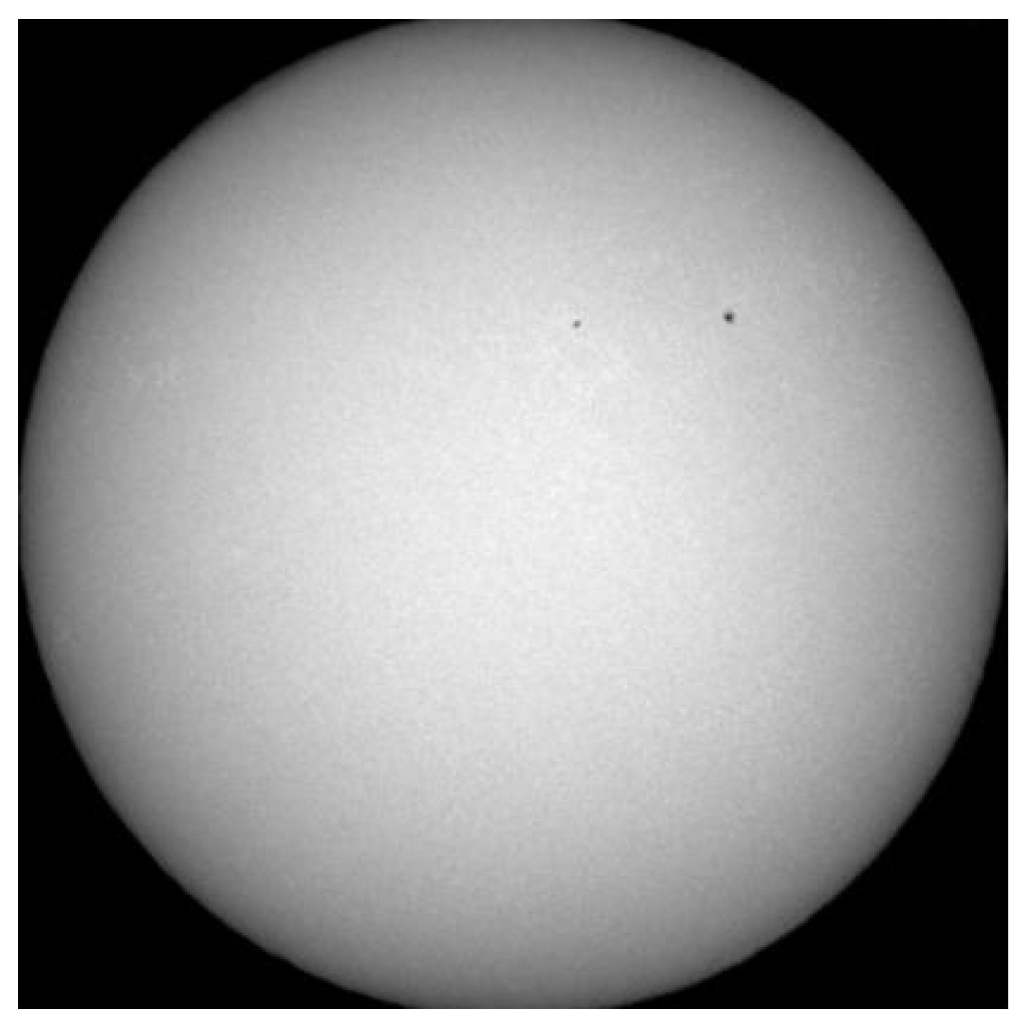
Figure 1 shows a good image, after removing the identification text.
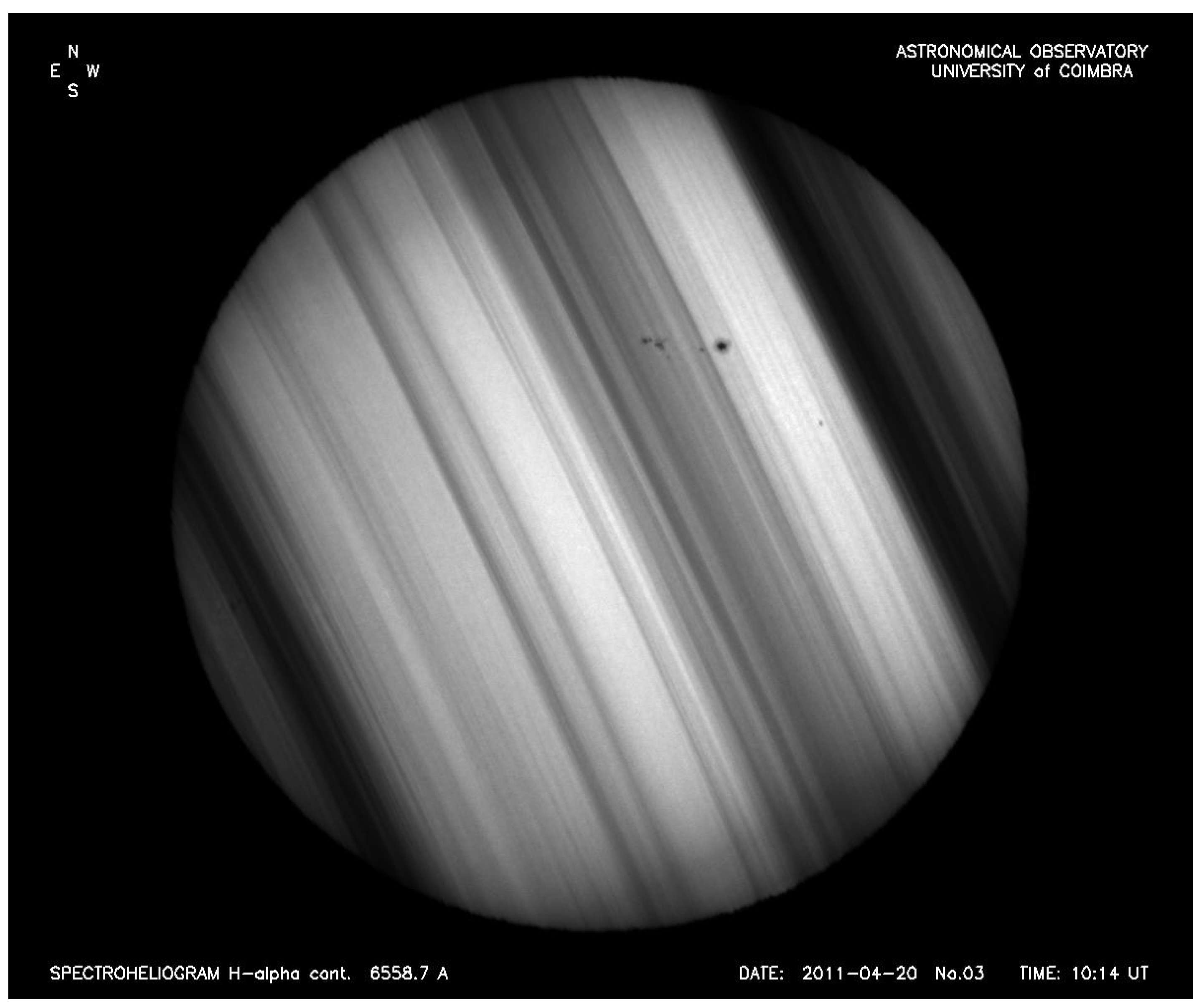
Figure 2 shows an example of a picture taken at the observatory, which is particularly challenging due to the bad weather that day. The picture clearly shows the slices due to the imaging process used, and it also contains its identification marking letters.
A previous work with images from the OGAUC performed sunspot detection using an algorithm with mathematical morphology to detect sunspots and facular regions [
9,
24]. The dataset consists of images taken from the spectroheliograph of OGAUC. In this work, the goal was to develop one method to apply to all the images captured at the OGAUC. Two methods to detect sunspots were considered:
Both methods were applied to a subset of images with features and other characteristics identified visually by an experienced solar observer. The work was based on an subset of images, consisting of 144 spectroheliograms. Those were 8-bit images of the solar cycle 24, spread over several years and different seasons. Image dimensions are 1200 × 1000 pixels.
As a first step, images were submitted to a pre-processing that consisted of a series of filters that, in addition to making the image easier to read by the algorithms, identified the solar disk [
9]. The filters applied were the following:
Morphological operation closing to make the image more homogeneous.
Morphological operation opening to remove letters from the image. Those letters are added to the original images to mark them, and contain information, such as date.
Subtraction of the resulting image from the original image (as a mask).
Morphological reconstruction of the image obtained as a mark.
Application of an adaptive threshold filter with a lower cutting value of 30 and an upper cutting value of 124.
Application of a morphological gradient called thinning, to obtain the contour of the sunspot.
The mathematical morphology-based method takes the pre-processed images as input, and filters and processes the image in order to output the contour of the sunspots and its penumbra. The threshold is defined by the average value between the maximum and minimum gray levels inside the sunspot. If the pixel value is lower than the threshold value, then it will be considered the umbra (the central part of the sunspot); otherwise, it will be considered the penumbra (the grayish outer part).
The second approach is based on the intensity of the digital level of the pixels, designated by PI. It consists of a two-stage process comprising (i) intensity normalization of the original image, and (ii) a sunspot detection stage, with the segmentation of umbra and penumbra. The goal is to create a synthetic image, in which the solar disk presents homogeneous digital levels and the background has a digital level of zero. This approach uses the same pre-processing as the first one presented. Using simple equations, the authors could also locate the center of the sunspots detected.
The results reported from the approaches mentioned are 86.25% for the mathematical morphology approach, and 84.32% for the pixel intensity approach.
3.2. Deep Learning for Automatic Recognition of Magnetic Type in Sunspot Groups
Fang et al. [
25] developed a deep learning algorithm to detect magnetic type in sunspot groups. Although the article focuses on the recognition of magnetic fields, a recognition of the sunspots themselves was needed. The authors constructed three models, which differ in the input content, that consist of the following:
Model A: magnetograms, images built from the detection of the intensity and polarity of the magnetic fields over the solar surface, where the sunspots are also detected but with the extra information on the polarity of the magnetic field;
Model B: SDO/HMI continuum images;
Model C: two-channel pictures.
The datasets used in the study consist of images collected by SDO/HMI (Solar Dynamics Observatory/Helioseismic and Magnetic Imager) and SHARP (Spaceweather HMI Active Region Patch) data, taken between May 2010 and May 2017. The data include magnetograms and continuum images with the time period of 12 min and location range of
heliolongitude degrees from the solar disk center, in order to reduce the influence of projection [
25]. In the active region, in order to ensure sufficient variations between the nearest images, the data are obtained every 96 min.
This way, the gray value of the pixel point with magnetic field strength greater than or equal to the maximum (800.0) obtains the value of 255; on the other hand, the gray value of the pixel point with a magnetic field lower than or equal to −800.0 is given the value of zero [
25]. The resulting pictures are interpolated into a uniform size of 160 × 80 pixels, to match the input size required by the CNN. After data processing, the CNN is trained using the dataset.
The CNN has good performance in the identification of the active region magnetic types. The overall accuracy of all three models is over 87%, and the total accuracy reaches over 95%. The accuracy for the Alpha type reaches 98% and the recognition accuracy for the Beta type always has values above 88%.
3.3. Detecting a Predefined Solar Spot Group with a Pre-Trained Convolutional Neural Network
Camargo et al. [
26] detected sunspots doing some pre-processing and using a CNN developed for sunspot and sunspot group characterization and classification. The dataset consists of 853 images, generated from 72 images from the HMI, in Intensitygram Flat format to allow easier manipulation of the image, which facilitates the pre-processing mentioned above. Regarding the dataset partition, 600 out of the 853 figures were used for training, while the other 253 were used for the testing phase.
Before being fed to the CNN, the images were pre-processed. The pre-processing consisted of the following steps:
- 1.
Image adjust (contrast stretching): method used to increase the contrast of the output image;
- 2.
RGB to gray: converts the RGB images into gray level images (uni-dimensional scale);
- 3.
Image to black and white: considering a threshold, the image is converted to a binary matrix, where the values above the threshold are converted to white, while the pixels below the threshold are converted to black;
- 4.
Image open (growth): this method performs an erosion followed by a dilation on the gray scale or binary image, using the same structuring element for both operations;
- 5.
Image complement: computes the complement of the image, inverting black and white colors;
- 6.
Region properties: used to measure a set of priorities for each connected object in the binary image;
- 7.
Image crop: obtains a region of an image in determined coordinates, within a box of certain dimensions;
- 8.
Image write: writes an image with a name specified by the user, in the determined format, in the current folder.
The authors present an example of the pre-processing stage, showing the resulting image of each step mentioned above, and including the final result with the detection of the sunspots.
3.4. Hierarchical Method for Quick and Automatic Recognition of Sunspots
Ziliang et al. [
20] proposed to develop a neural network based on YOLOv3, for the automatic recognition of sunspots. The dataset used consists of 700 continuum images obtained from SDO/HMI dataset for training, and continuum images randomly selected from 2010 to 2014 for testing.
The final result shows that the entire processing flow achieves a 73.41% intersection ratio, 98.50% recognition rate and 0.60% false recognition rate. Regarding the recognition speed, this approach obtained much better results in comparison to other sunspot recognition algorithms.
3.5. Fast Solar Image Classification Using Deep Learning and Its Importance for Automation in Solar Physics
Armstrong et al. [
27] proposed a CNN for the classification of solar images, composed of 13 layers, characterized as one of the following types: convolutional, pooling and dense layers. Images obtained from Hinode Solar Optical Telescope (SOT) are analyzed by the mentioned neural network and classified into one of five classes: filaments, flare ribbons, prominences, sunspots, and quiet sun (absence of the previous four).
The dataset was divided into training set and validation set. The training set consists of 11,857 images from the SOT, classified manually into one of the classes mentioned above. The validation set consists of 1318 Hinode/SOT images spread approximately equally between the classes. There is a total of 13,175 images used in the whole project.
Regarding the initialization of the network, in order to reduce the number of training epochs, He initialization was employed.
The optimization method used was SGD with Nesterov momentum, which is similar to the standard but has an additional parameter: velocity. This ensures better performance for the network.
To improve the network stability and normalize the output of the convolution calculation, “batch normalization” was applied to the convolution operation’s output. Additionally, to avoid the vanishing gradient problem, Armstrong et al. used the rectified linear unit (ReLU) function. Maxpooling layers are used for downsampling the data in order to increase processing performance by reducing the number of parameters. The downsampling works by converting the image into square grids of 2 × 2 pixels. This results in a new image in which each pixel represents four pixels of the input image. For the training phase, the loss function used is the “cross entropy loss”, which is based on the discrete version of a multinomial logistic regression.
The results obtained were very satisfactory, as the CNN reached an accuracy of 99.92%, which means that only 1 out of the 1318 images was misclassified.
3.6. Automatic Analysis of Magnetograms for Identification and Classification of Active Regions Using Deep Learning
Oliveira et al. [
28] proposed a deep learning technique in Python for the detection and classification of active regions. Several deep learning models were taken into account in order to compare the results between them and find the one(s) with the best accuracy. The goal of the methods developed was to classify the solar flares as one of the classes shown in
Table 1.
The dataset was obtained from The Helioviewer Project (2019) (
https://helioviewer.org/, accessed on 5 May 2023). The data were divided into two sets, according to the neural network to be trained. For the detection algorithm, 1000 magnetograms (that were labeled using Fiji software, with the ALP plugin) were used to train the first neural network. For the classification algorithm, the dataset consisted of 1548 images, divided into classes characterized by the magnetic configurations:
Each sub-dataset was also divided into a training set (70% of the total dataset), validation set (20%), and test set (10%).
Since the dataset did not include the classification for all the sunspots found, two neural networks were created: one only for the detection of sunspots and the other for classifications of the sunspots found. The neural networks used were feed-forward supervised learning networks. The best model developed for the detection of the active regions reached a maximum accuracy of 80.75%, while for the classification algorithm, the best model reached a maximum level of 88%.
3.7. Sunspot Identification and Tracking with OpenCV
Toit et al. [
29] reported the development of a neural network for the identification and tracking of sunspots. It is split into two phases that consist of each of the goals of the neural network mentioned.
The dataset consists of ten continuum images taken in February 2014. Due to the fact that the solar cycle was at its height for sunspot generation, this was determined to be the ideal moment. The images went through a pre-processing phase that consisted of the following:
Filtering phase: This process consists of removing the noise from the image and detecting the solar disk, as well as its radius and center. It includes the creation of the mask that is used in the filtering process. With the use of some equations, it is possible to calculate the position angle, latitude and heliographic longitude.
Correlation phase: in this phase, magnetogram images are used to correlate both magnetogram and Michelson Doppler images (MDI) from the first stage.
The method reached an accuracy of 88.4% in sunspot detection.
3.8. Other Approaches
Besides the approaches described, there exists other research toward automating the process of detecting sunspots in digital archives. Bibhuti et al. work with images from the Kodaikanal Solar Observatory, which allegedly possesses solar images since 1904 [
30].
Alasta et al. use PICARD satellite images to detect and calculate the filling factor of sunspots [
31]. E. Fini proposes a method to detect and count sunspots using a model based on U-net deep convolutional neural network [
32]. Quan et al. compare the performance of R-CNN and YOLOv3 to detect sunspots in HMI SDO images [
33]. Soler et al. propose a method to predict the evolution of sunspots, based on light bridges, using deep learning methods [
34].
3.9. Summary
As shown previously, space weather is very important for life on Earth; thus, the area of sunspot detection has been subject to heavy research. Spectroheliograph images have been available for almost a century, so they keep a long record of the history of the sun. Modern satellite images have higher quality, but they record only the last few decades.
Hence, the following research questions remain open, and answers are sought in the present work: (i) How can deep learning methods be used to detect sunspots in spectroheliograph images from the OGAUC database? (ii) What is the best performance achievable in sunspot detection with one modern and fast CNN model, namely YOLOv5?
4. Materials and Methods
Experiments for the present work were performed using a dataset of OGAUC images and an open source implementation of YOLOv5.
4.1. Data Sets of Selected Images
The set of images used for the present work consisted of 2000
continuum images, with resolution 1200 × 1000 pixel. Those images were taken at the OGAUC spectroheliograph, between 15 February 2012 and 26 April 2019, so they correspond to solar cycle 24. They were obtained from the public repository Bass2000 Solar Survey Archive (
https://bass2000.obspm.fr/ accessed on 26 April 2023). The images contain the solar disk and side annotations, as shown in
Figure 2. As happens with images taken from the earth’s surface, the quality depends on the atmospheric conditions of the day they were taken. That means the quality of the images is not always the same.
Figure 2 in particular shows an image that was taken in a cloudy day, so the quality is very poor and only the larger sunspot is clearly visible. Additionally, the images were captured using a composition process that sometimes results in images shown as a number of different slices. Those characteristics make them harder to analyze than other sun images, especially those taken from outer space by satellites or telescopes in orbit, where there is no influence of the earth’s atmosphere.
Throughout the study, a number of different experiments were performed in order to determine the best image-marking methods and parameters of the YOLO models, as well as the pre-processing methods to be used. Therefore, six different smaller datasets were created, named A to F, to perform different experiments. The main difference between datasets is the number of images. Smaller datasets were created for faster experiments and larger datasets for more accurate results. A more detailed description is as follows:
Dataset A—a small subset, to experiment with the annotation software and create the first models. It consists of 50 images, which were expanded to 120 using data augmentation methods, namely flip, rotate and shear.
Dataset B—consists of 932 images, expanded to a total of 2076 through data augmentation processes flip, rotate and shear.
Dataset C—a total of 1000 images, expanded to 2379 through data augmentation processes. This dataset was created in order to experiment with more precise annotation of the dataset.
Dataset D—dataset of cropped images. The frame around the solar circle was removed so that only the relevant part was maintained. From 500 spectroheliograms, 958 images were generated through data augmentation processes, in this case, just flipping the image.
Datasets E and F—created as the final dataset for the work. Dataset E is the first half of the final dataset, which is dataset F. The first and second halves of dataset F consist of 1919 and 1928 images, respectively, generated from 1000 images each, through data augmentation processes (again, just flipping).
For datasets D, E and F, the images were cropped in order to reduce the pixel loss when scaled for the network input. Cropping consisted of removing the letters and most of the black area around the sun disc, leaving just the relevant area. Cropping removes data which are not relevant and also makes the sunspots larger and easier to identify, so this pre-processing step was assumed important and used in the final experiments.
Dataset F is divided into train and validation sets with 3247 and 600 images, respectively.
4.2. Experimental Setup
YOLO is a state-of-the-art deep neural network in object detection [
20]. Therefore, it was the framework chosen for the present implementation. Namely, the PyTorch implementation YOLOv5 (
https://github.com/ultralytics/yolov5 (accessed on 5 May 2023)), which has a number of different versions available. Some of those versions are smaller and faster, while others are larger and require more computation resources. The versions tested for the present work were YOLOv5s (small), YOLOv5m (medium) and YOLOv5l (large).
The datasets were organized, marked and managed using the Roboflow (
https://app.roboflow.com/ (accessed on 5 May 2023)) framework. Training was performed using Google Colaboratory (
https://colab.research.google.com (accessed on 7 May 2023)), a tool with an environment similar to Jupyter Notebook that provides computing resources from Google servers, such as GPU, which is ideal for training deep neural networks, such as YOLOv5. The notebook was started from a template provided by Roboflow Model Zoo (
https://models.roboflow.com/object-detection/yolov5 (accessed on 7 May 2023)).
4.3. Performance Metrics
The main performance metrics used for assessment of the model are precision (
P) and recall (
R). Precision is a measure of the predictive value, and recall is also known as a measure of the sensitive value. They are defined as follows:
In the equations, means true positive, means false positive and means false negative.
Another performance metric used is mean average precision (), which is the average precision of the model when a given threshold is imposed for detection. A threshold of 0.5, for example, requires that the bounding box of a sunspot detected by the network overlaps at least 50% with the bounding box designed when marking the dataset.
5. Experiments and Results
The results obtained show that YOLOv5 is able to detect a large percentage of the sunspots, despite the difficulties posed by the quality of some of the spectroheliograms.
5.1. Experiments with Different Datasets
Several training experiments were performed, with the different datasets described in
Section 4.
Table 2 shows a summary of the main experiments, including the relevant parameters and the results obtained.
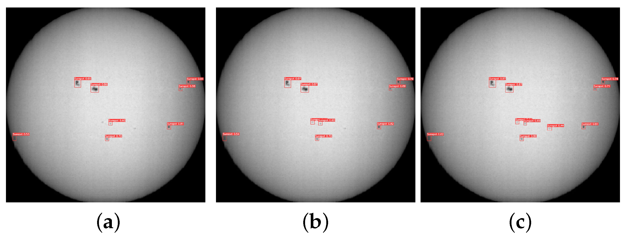
The table shows the results of various experiments performed in order to determine the best values for the hyperparameters. The first experiment had the purpose of evaluating whether the YOLO model was learning, or how fast it was learning. The result was very unsatisfactory due to the small amount of images to train with, but it still showed the ability of the model to learn and achieved a precision of 33.33% after 73 epochs with a batch size of 12. Example of the sunspot detection using the best weights obtained with the various network structures L, M and S show in
Figure 3.
Using dataset B, three different experiments were performed in order to glean insight into the performance of each method and determine the best one for the present problem. The methods were as follows:
Standard train—consists of a 200 epochs training;
Incremental train—the weights generated by a training experiment are used in the following one, counting up to three instances;
Train with several steps—the batch size starts large and then decreases;
Dataset C was used for a single experiment. The results were apparently good since the precision was over 90%. However, that was at the cost of data augmentation. For better confidence in the results, more images were marked later, and larger datasets were constituted.
Dataset D was used to test different pre-processing methods, as described in
Section 4. First, the images were cropped, removing the frame around the solar disk. The results obtained with the cropped images were good and stable between different runs, even though the dataset was small. From this point on, the experiments were performed using cropped images. The table shows that the other pre-processing methods brought no improvement to the results. In some experiments, there were good results, but they were not repeatable; thus, they probably show that pre-processing can actually make the process more unstable.
The last experiments were performed with 1000 marked images, which were used to make datasets E and F. Dataset E was used to test whether there was a significant advantage using more annotated images. The results show that the YOLO model was able to achieve some of the best precision rates, and the results were repeatable, with only minor variations between each run. Afterward, more experiments were performed, using the same images and adding more data augmentation techniques, thus producing dataset F. As the table shows, there is no significant advantage in adding more images through data augmentation.
As the results show, the standard training method is able to achieve good results, and the results are, in general, stable and repeatable. There are differences in the results because the initial conditions are random and, therefore, the learning process may converge faster or slower, or even converge to the local minima. Some experiments were run more than once in order to minimize the influence of random results in the conclusions.
5.2. Discussion
In the first experiments, although many tests reached good precision rates, they were achieved very early in the training process and they were not always repeatable in other test sets. This likely happened because the datasets were too small, so the results were mostly randomly overfit to those particular samples. The experiments show that a minimum of 1000 manually annotated images were necessary to train a robust model and have some confidence in the results obtained.
The results also show that YOLO benefits from images that are as large as possible. When the frames and annotations around the images were removed, the performance improved significantly. Processing the images using contrast enhancing techniques did not contribute to improving the results.
The results above were obtained using the smallest model of the YOLOv5 family, which is YOLOv5s. Additional experiments were performed with more powerful models, namely the m and l versions. A comparison of the relevant results is shown in
Table 3.
The results presented show the main differences between the YOLO models. The table shows the best precision, recall, objectness (Obj) and mean average precision (mAP) with confidence 0.5 and 0.95. It also shows the time required to train each model. As the table shows, the larger models have a slightly better precision. However, that comes at the cost of much longer training times. This may be an obstacle for training with larger datasets. For inference, however, that problem is less important because the network only needs to process each image one time.
The results obtained in the present experiments are inferior to many described in
Section 2. However, other authors use images which are obtained using satellites or telescopes in outer space. Images obtained from space do not suffer from atmospheric conditions. They are cleaner, clearer and show the sunspots in greater detail. The atmosphere adds different types of noise to the images, where many particles in the air interfere with the light coming from the sun, absorbing or reflecting part of it.
Comparing to previous work that uses images from the OGAUC, namely Carvalho et al. [
9], the YOLOv5 neural network achieved a slightly higher detection accuracy on a much larger dataset, even though the version implemented will only return the bounding box and not additional spot information. Additional information, such as the sunspot area or umbra, as reported by Carvalho et al., may be detected by segmentation models.
Table 4 shows a summary of the best precisions reported by Carvalho et al., using mathematical morphology, pixel intensity, and the YOLO models. YOLOv5s offers a precision which is 2.60% higher than the mathematical morphology method, and YOLOv5l has a precision 1.15% higher than the smaller architecture. It should be noted that all the images used in all the tests are from the same OGAUC dataset and the same solar cycle. Nonetheless, the subset used by Carvalho et al. is smaller than the subsets used for the experiments with YOLO models, in part because training for deep neural networks requires larger numbers of samples when compared to mathematical morphology and pixel intensity models.
Compared with other authors, for example, Fang et al., described in
Section 3, the precision of the YOLO models is lower. Fang et al. achieved up to 98%. Ziliang et al. achieved 98.5%. Armstrong et al. achieved 99.92%. The difference comes from the different types of images used—Fang et al. used images taken from space, while the OGAUC image are taken from Earth.
Other approaches achieve more modest results, comparable to those obtained in the present work. For example, Oliveira et al. and Toit et al. reported up to 88% precision.
5.3. Main Contributions
The present work offers several contributions to the state of the art. The research questions proposed in
Section 3 are answered. The most important contributions are listed below.

 ,
, 


