Article

Parallel Frequent Subtrees Mining Method by an Effective Edge Division Strategy

1
School of Media Science, Northeast Normal University, Changchun 130024, China
2
Key Laboratory of Symbolic Computation and Knowledge Engineering of Ministry of Education, Jilin University, Changchun 130012, China
*
Author to whom correspondence should be addressed.
Appl. Sci. 2022, 12(9), 4778; https://doi.org/10.3390/app12094778
Submission received: 13 April 2022 / Revised: 4 May 2022 / Accepted: 6 May 2022 / Published: 9 May 2022
(This article belongs to the Special Issue Data Analysis and Mining)

Abstract

:
Most data with a complicated structure can be represented by a tree structure. Parallel processing is essential to mining frequent subtrees from massive data in a timely manner. However, only a few algorithms could be transplanted to a parallel framework. A new parallel algorithm is proposed to mine frequent subtrees by grouping strategy (GS) and edge division strategy (EDS). The main idea of GS is dividing edges according to different intervals and then dividing subtrees consisting of the edges in different intervals to their corresponding groups. Besides, the compression stage in mining is optimized by avoiding all candidate subtrees of a compression tree, which reduces the mining time on the nodes. Load balancing can improve the performance of parallel computing. An effective EDS is proposed to achieve load balancing. EDS divides the edges with different frequencies into different intervals reasonably, which directly affects the task amount in each computing node. Experiments demonstrate that the proposed algorithm can implement parallel mining, and it outperforms other compared methods on load balancing and speedup.

1. Introduction

The era of big data has arrived with the advent of massive data. Semi-structured data [1,2] plays a crucial role in massive data with the non-strict structure feature. Most data with a complicated structure, including semi-structured data, can be represented by a tree structure. Data mining methods are used to find hidden relationships among massive data [3,4]. Frequent subtree mining has become an important field of data mining research [5,6,7]. It is the process of mining a subtree set from a given data set that satisfies user attention (support or frequent degree). Frequent subtree mining can be applied in many fields. For example, RNA molecule structure can be represented by a tree structure where, in order to obtain information about a new RNA molecule, the new one must be compared to the known RNA structures. The function information of new RNA can be obtained by looking for the same topology [8].
CFMIS (compressed frequent maximal induced subtrees) [9] is an efficient method for the frequent subtree mining we proposed earlier. The CFMIS algorithm can find all frequent induced subtrees without throwing solutions in less time. Parallel frequent subtree mining processing is essential for mining massive volumes of data in a timely manner. MapReduce is an ideal software framework to support distributed computing on large data sets on clusters of computers [10,11]. However, not all algorithms could be transplanted to the MapReduce framework, in fact, only a few algorithms could. Assigning data into appropriate blocks is crucial for paralleling algorithms in MapReduce [12]. In this paper, three parallel CFMIS (PCFMIS) algorithms, PCFMIS1, PCFMIS2 and PCFMIS3, are proposed. PCFMIS1 parallels CFMIS, transplanting CFMIS to MapReduce framework by GS. Furthermore, PCFMIS2 is proposed by optimizing the compression to reduce the running time on each slave node. Based on PCFMIS1 and PCFMIS2, PCFMIS3 is proposed to achieve load balancing by using an effective EDS.
In summary, the contributions of our work are as follows:
1.
A grouping strategy is proposed to achieve effective data partitioning in order to parallel the frequent subtrees mining method.
2.
The compression is optimized by avoiding all candidate subtrees to reduce the mining time on nodes.
3.
An effective edge division strategy is proposed to achieve load balancing.
4.
The proposed algorithm PCFMIS3 is outstanding on load balancing and running time.
The rest of the paper is organized as follows: in Section 2, related work is reviewed; the proposed PCFMIS1, PCFMIS2 and PCFMIS3 are presented in Section 3; in Section 4, experimental results are displayed and discussed; conclusions are made in Section 5.

2. Related Work

With the extensive application of semi-structured data, the research priority of frequent pattern mining has expanded from frequent item set mining [13,14] to frequent subtree mining [15]. L. Wang et al. proposed a novel framework for mining temporal association rules, which mainly represent the temporal relation among numerical attributes [16]. A new structure called a frequent itemsets tree is proposed to avoid generating candidate item sets in mining rules. Building the tree and mining the temporal relation between the frequent itemset proceed simultaneously. V. Huynh et al. proposed an improved version for IPPC tree, called IPPC+, to increase the performance of the tree construction [17]. IPPC+ improves the poor performance of IPPC tree in the case of datasets comprising a large number of distinguishing items but just a small percentage of frequent items. W. Pascal et al. proposed an algorithm mining probabilistic frequent subtrees with polynomial delay, but by replacing each graph with a forest formed by an exponentially large implicit subset of its spanning trees [18]. The algorithm overcomes the drawback that the number of sampled spanning trees must be bounded by a polynomial of the size of the transaction graphs, resulting in less impressive recall even for slightly more complex structures beyond molecular graphs. J. Wang et al. proposed a compression tree sequence (CTS) to construct a compression tree model and saved the information of the original tree in the compression tree. CFMIS [9] was proposed based on CTS to mine frequent maximal induced subtrees. For each iteration, compression could reduce the size of the data set, thus, the traversal speed was faster than that of other algorithms.
Out of memory and computing resources lead massive data mining to difficulties. Parallel data mining can be an effective solution to this problem [19,20,21]. In recent years, researchers have made some achievements in frequent item mining. S. Shaik et al. presented a scalable parallel algorithm for big data frequent pattern mining [22]. Three key challenges are identified to parallel algorithmic design: load balancing, work partitioning and memory scalability. D. Yan et al. proposed a general-purpose framework PrefixFPM for FPM that is able to fully utilize the CPU cores in a multicore machine [23]. PrefixFPM follows the idea of prefix projection to partition the workloads of PFM into independent tasks by divide and conquer. The state-of-the-art serial algorithms are adapted for mining frequent patterns including subsequences, subtrees, and subgraphs on top of PrefixFPM. D. Yan et al. extend PrefixFPM to provide the complete parallel algorithms by adopting four new algorithms so that a richer set of pattern types are covered, including closed patterns, ordered and unordered tree patterns, and a mixture of path, free tree, and graph patterns [24]. PrefixFPM exposes a unified programming interface to users who can readily customize it to mine their desired patterns. Xun. Y. et al. proposed FiDoop to achieve compressed storage and avoid building conditional pattern bases [25]. Hong T. P. et al. proposed a parallel genetic-fuzzy mining algorithm [26] based on the master–slave architecture to extract both association rules and membership functions from quantitative transactions. C. FB et al. proposed a frequent itemset mining method using sliding windows capable of extracting tendencies from continuous data flows [27]. They develop this method using Big Data technologies, in particular, using the Spark Streaming framework enabling distribution of the computation along several clusters and thus improving the algorithm speed. Sicard. N. et al. proposed a parallel fuzzy tree mining method (PaFuTM) [28]. In some of their approaches, the level-wise architecture is preserved but tasks are parallelized within each level. All candidates from each frequent subtree are assigned to specific tasks where they are generated and tested against the database.

3. PCFMIS Algorithm

In this section, we provide the definitions for some concepts that will be used in the remainder of the paper. The proposed parallel algorithm will also be explained in detail.

3.1. Prepared Knowledge

3.1.1. Definitions for Concepts

The CFMIS algorithm deals with the tree in which sibling nodes are unordered with labels and the sibling nodes of the same parent node have no repeats. The ‘tree’ mentioned below is the same tree as the CFMIS processes, assuming that there is no repeat label in a same tree. CFMIS focuses on frequent maximal induced subtree mining.
 Definition  1. 
Induced subtree. A tree T = ( V , E , r ) is an induced tree of T = ( V , E , r ) , denoted as T T if V V , E E , where V is the set of nodes; E is the set of edges in which ( x , y ) E represents that x is the parent of y; r is the root node.
 Definition  2. 
Frequent subtree. D = { T 1 , T 2 , , T n } is a tree set, ε is the frequency threshold, O c c ( T i , T ) represents whether T occurs in T i , if T T i , then O c c ( T i , T ) = 1 , else O c c ( T i , T ) = 0 . F r q ( T ) = i = 1 n O c c ( T i , T ) . T is frequent subtree if F r q ( T ) ε .
 Definition  3. 
Maximal subtree. F is the frequent subtree set of D. T and T are two frequent subtrees in F, T maximize T (denoted as T m T ) if and only if T T , there is no T in F to make T m T happen. T is called maximal subtree.
 Definition  4. 
Compression tree sequence(CTS). CTS is an ordered sequence composed by n o d e p d , C T S = ( n o d e 0 p d 0 , n o d e 1 p d 1 , , n o d e n p d n ) , p d is the index pointing to the parent node for each node except the root node. Let the parent of n o d e i p d i be n o d e j p d j , and then p d i = | i j | , where n o d e 0 p d 0 is the root node.
For example, the CTS of the example tree in Figure 1 can be a 0 b 1 c 2 d 1 e 2 f 3 . a 0 is the root element. a is the parent element of b, due to the difference between the positions of a and b in the CTS is 1 while the index superscript of b is 1. c is the parent element of f, due to the difference between the positions of c and f in the CTS being 3 while the index superscript of f is 3. The same rule applies to other nodes, so the information about tree structure and all the edges in the tree can be obtained from CTS.
 Definition  5. 
Tree list length. The number of n o d e p d in CTS is the length of CTS.

3.1.2. CFMIS Algorithm

A simple review of the CFMIS algorithm is described below (more details in [9]), and it is primarily performed via four stages:
Stage 1. Construct the compression tree model: the original data set is constructed as a compression tree model using CTS;
Stage 2. Cutting edge: this stage is divided into two subprocesses, trim edges and clean-up edges. First, trim the edges for which the edge frequent degree is less than threshold. Then, delete the single node.
Stage 3. Find frequent subtrees: Compress them according to the descending edge frequent degree to obtain CTSs, and sort CTSs according to the tree list length from shortest to longest. Match the C T S i with the CTSs following it; if matched (the C T S i is obtained in another C T S j ), then the frequent degree of the T represented by C T S i is incremented by 1.
Stage 4. Maximal Stage: Run the frequent subtree sets maximal processing. The frequent maximal induced subtree set of the original data set are obtained.

3.2. Grouping Strategy

Data partitioning is the premise of the parallel algorithm. An effective data partitioning method can greatly reduce the data communication between different slave nodes, thereby reducing the parallel computing time. Based on the above findings, the grouping strategy (GS) of PCFMIS used to divide all the trees in original data set D into different groups is described below:
(1) If given m slave nodes, we should divide all the trees in D into m groups, and the number of the group is denoted as G n u m . For the edge (x,y) in D, divide (x,y) into the set A = { A k } , k [ 1 , m ] .
(2) For T i D , all the edges in T i may belong to several A k according to (1). Take the minimum of these k as the G n u m of T i , G n u m = min k, so T i is put into the group which G n u m = min k. Then, for T i , cut the edges which belong to A m i n k . Some new trees T i will appear after cutting edges.
(3) For these new trees T i , repeat (2) until no new trees are produced.
(4) For T j D , repeat (2) and (3).
(5) All the trees in original data set D are divided into different groups, and the different groups will be put in different slave nodes.
 Definition  6. 
Related Tree. Given a tree T = ( V , E , r ) , for ( x , y ) E , there is ( x , y ) A k . min k is the minimum of k. When ( x , y ) A m i n k , T is a related tree of ( x , y ) , denoted as ( x , y ) T . The set of t ( x , y ) T is denoted as Γ ( x , y ) .
 Property  1. 
According to grouping strategy, a tree in original data set only belongs to one group.
 Property  2. 
According to grouping strategy, if ( x , y ) A k , all Γ ( x , y ) will be put into the group which G n u m = k .
According to Property 1, the trees in the original data set are grouped into different groups, which can reduce the scale of the data each slave node needs to process. Although in (2), new trees may be generated during the grouping process, the new trees are trimmed and less complex than the original tree.
We can conclude from Property 2, for ( x , y ) A k , all the induced subtrees of Γ ( x , y ) containing ( x , y ) can be found in the group in which G n u m = k . So frequent induced subtrees of Γ ( x , y ) containing ( x , y ) can be found only in group k instead of the whole original data set. This avoids communication between groups and realizes real parallelism.
 Definition  7. 
Frequent Edge Degree. D = { T 1 , T 2 , . . . , T n } , the frequent edge degree of ( x , y ) is the number of times ( x , y ) appears in D, denoted as E F r q ( x , y ) .
How to divide the edge ( x , y ) into set { A k } in (1) directly affects the G n u m of Γ ( x , y ) . One feasible method is described below:
Given an evenly divided interval A d i v = ( a 1 , . . . , a i , . . . , a m ) , a 1 > . . . > a i > . . . > a m , a 1 = E F r q m i n ( x , y ) , a m = E F r q m a x ( x , y ) . If a i + 1 > E F r q ( x , y ) a i , the edge ( x , y ) is divided into A i , then Γ ( x , y ) will be put into the group in which
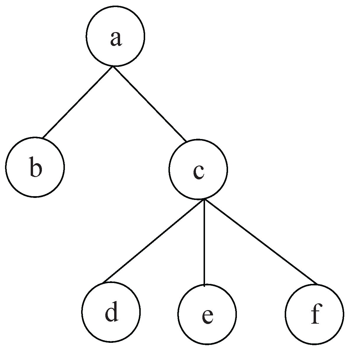
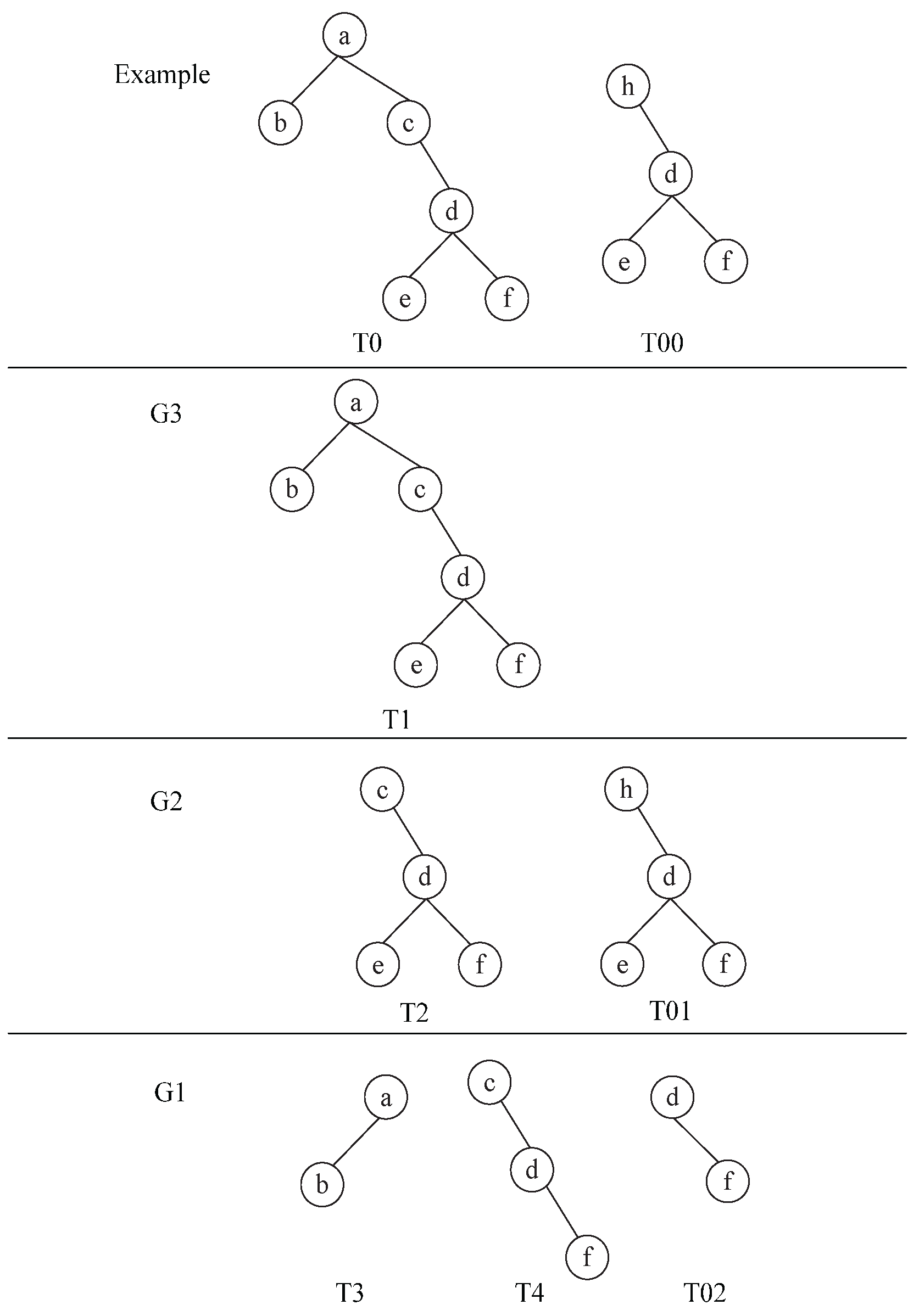
 G n u m = k . For example, in Figure 2, suppose that the number of slave nodes is 3. Divide the trees T 0 , T 00 into 3 groups ( G 1 , G 2 , G 3 ) . Given dividing interval A d i v = ( a 1 , a 2 , a 3 ) , a 1 > a 2 > a 3 . E F r q ( a , b ) , E F r q ( c , d ) , E F r q ( d , f ) a 1 , a 1 > E F e q ( h , d ) , E F r q ( d , e ) a 2 , a 2 > E F r q ( a , c ) a 3 , so ( a , b ) ( c , d ) ( d , f ) are divided into A 1 ; ( h , d ) ( d , e ) are divided into A 2 ; ( a , c ) is divided into A 3 . Take T 0 in Figure 2 as an example. For A 3 , Γ ( a , c ) (in Figure 2) is divided into G 3 . Then delete ( a , c ) from A 3 and cut ( a , c ) . For A 2 , Γ ( a , c ) ( T i in Figure 2) are divided into G 2 . Then delete ( d , e ) from A 2 and cut ( d , e ) . For A 1 , Γ ( a b ) ( T 3 in Figure 2), Γ ( c d ) ( T 4 in Figure 2) and Γ ( d f ) ( T 4 in Figure 2) are divided into G 1 . T 01 , T 02 are obtained after applying GS on T 00 .
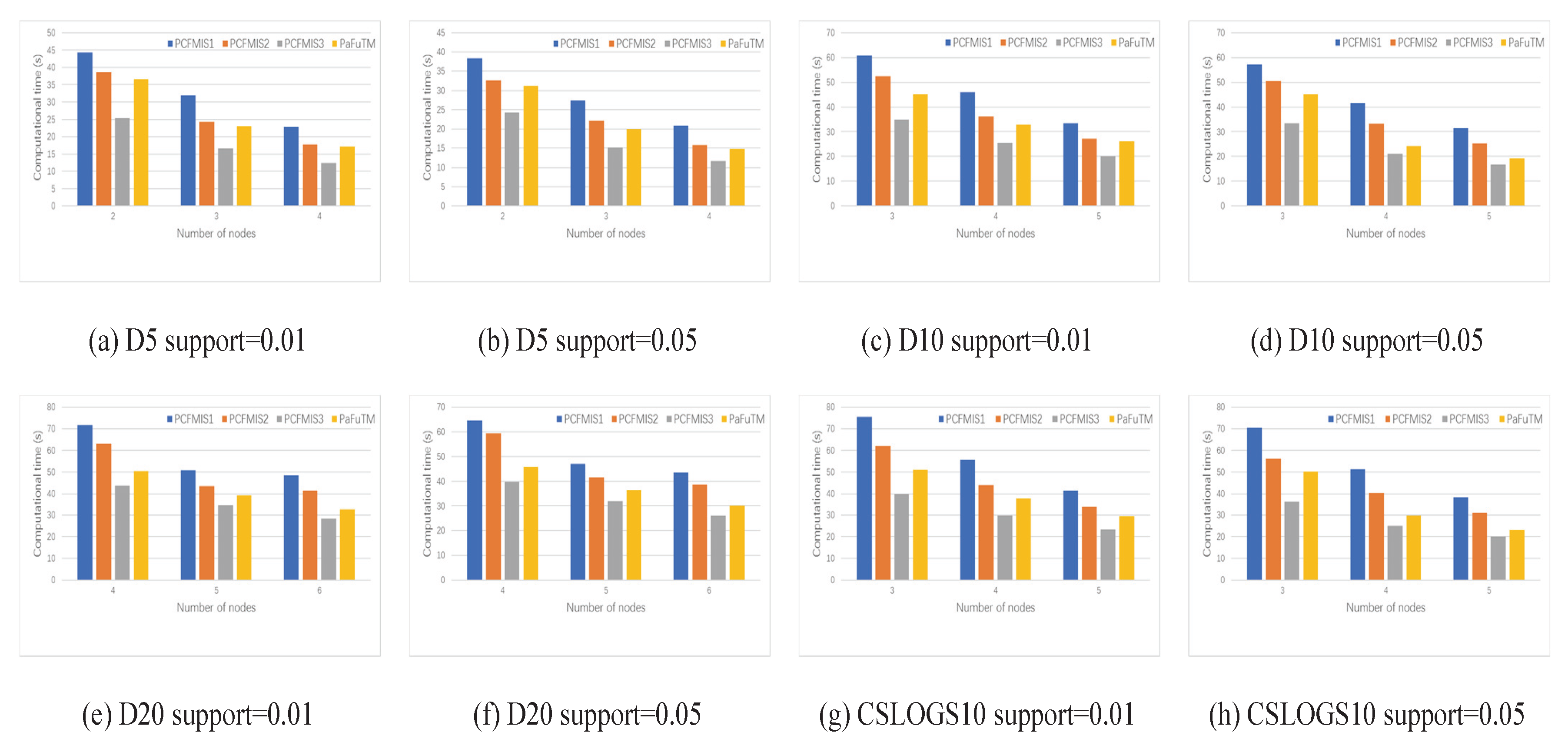
By using the above grouping strategy on the original data set and applying CFMIS algorithm in each group, the CFMIS algorithm is implemented in parallel. The new parallel algorithm is called PCFMIS1. However, the experiment results shown in Section 4.2 indicate that the parallel computing time and speedup did not achieve the desired results. Further improvements on PCFMIS1 will be discussed below.

3.3. Improvements on Parallel Algorithm

3.3.1. Optimized Compression in CFMIS

Stage 3 is the central step of the CFMIS algorithm, and it also takes most of the time in CFMIS. The subsequence processing of Stage 3 must find all subtrees of a compression tree to determine whether each of them is frequent. In fact, it consumes up to 70% of the execution time in this stage. Optimizing Stage 3 can greatly reduce time consumption of the algorithm, particularly when the data size is large. In this section, CFMIS is refined by optimizing Stage 3.
According to Property 2, for any edges ( x , y ) A k , all the induced subtrees of γ ( x , y ) containing ( x , y ) can be found in the group k, so frequent induced subtrees of γ ( x , y ) can also be found. For other edges ( p , q ) A k , ( p , q ) A f , all the induced subtrees of γ ( p , q ) containing ( p , q ) can be found in the group f. For the reasons above, we only need to find all the frequent induced subtrees of γ ( x , y ) which contain ( x , y ) instead of all the frequent induced subtrees in group k. Other frequent induced subtrees could be found in other groups. If a CTS in group k does not contain ( x , y ) , this CTS does not have to match with the CTSs following it. That is, this improvement in Stage 3 avoids finding all subtrees of a compression tree to determine whether each of them is frequent. The improvement in compression in groups makes the running time shorter. The improved parallel algorithm is called PCFMIS2. Although the time has been reduced, the load on slave nodes is not balanced.

3.3.2. Load Balancing

An effective edge division strategy (EDS) is proposed in this section. If ( x , y ) ϵ A k , Γ (x,y) will be put into the group k. The division of edges in the original data set affects the load of the slave nodes. Take the frequent edge degree as the basis for the edge division strategy. Abstract edge division strategy as a math problem, it can be described as below: Suppose that there are w different edges in the original data set, and their frequent edge degree is denoted as E F r q ( i ) , 1 ⩽ iw. Record E F r q ( i ) in the array x [ i ] . Divide different edges from the original data set into the set { A k } , ensuring that the sum of the frequent edge degree in each A k is approximately equal. The improved parallel algorithm is called PCFMIS3.
The steps of EDS are described below:
1.
Get the mean of array X, u= X [ i ] k .
2.
Traverse the array X, if X [ i ] > u, then it is assigned separately to a group. Suppose there are s groups like that.
3.
Now, the problem is translated into such a problem: divide ( w s ) different edges into ( k s ) sets, ensuring that the sum of the frequent edge degree in each group is approximately equal.
4.
For the rest X [ j ] , 1 ⩽ jws, get the mean of array X, u = X [ j ] k s .
5.
Translate the step (3) and (4) problem to 0–1 Knapsack Problem in order to solve it.
An example of the EDS method is given here to show how it works: suppose that the frequent edge degree of the original data set is 50, 60, 80, 100, 150, 200, 400, 1000, and k = 3. The mean value u =  50 + 60 + 80 + 100 + 150 + 200 + 400 + 1000 3  = 680. As 1000 > 680, 1000 is assigned separately to A 1 . Now, the problem is translated into such a problem: Divide the rest of the edges into two sets, ensuring that the sum of the frequent edge degree in each set is approximately equal. Get the mean value u =  50 + 60 + 80 + 100 + 150 + 200 + 400 2  = 520. Translate the problem to 0–1 Knapsack Problem in order to solve it. The weights of these items are 50, 60, 80, 100, 150, 200, 400 and the backpack capacity is 520. The answer is that 50, 60, 400 make the total value biggest in the backpack. 50, 60, 400 are assigned to A 2 , and the rest are assigned to A 3 .
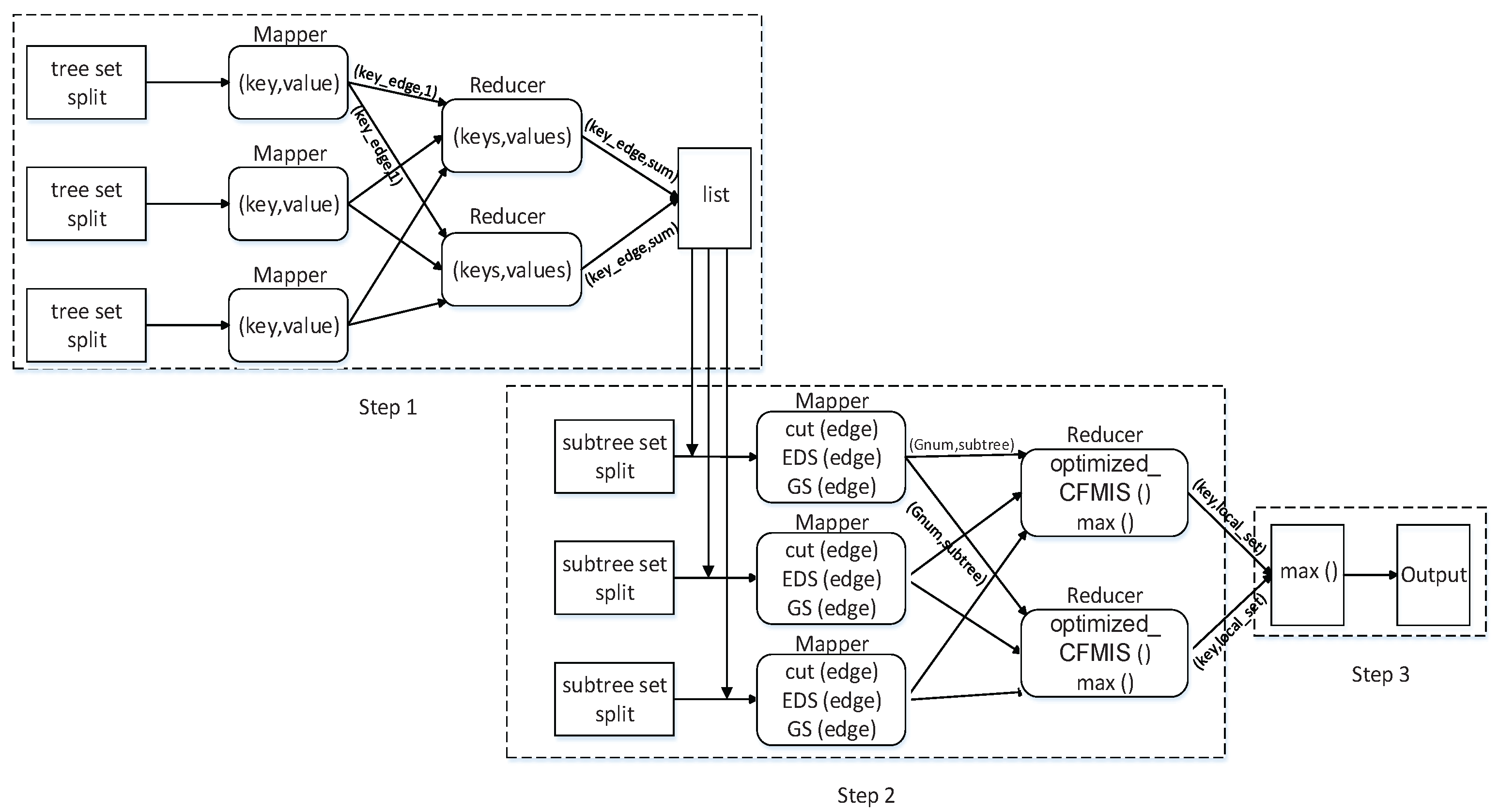
PCFMIS3 solved the problem of load balancing and introduced the optimized compression. The flowchart of PCFMIS3 is shown in Figure 3. Three steps including two Map-reduce operations are completed during parallel computation.
Step1: Calculate edge frequent degree of each edge in original tree set. In Map 1 (Algorithm 1), record each occurrence of each edge in a tree set split, which is the input of Reduce 1 (Algorithm 2). In Reduce 1, the edge frequent degree of each edge is counted out.
Step 2: Cut edge and find frequent subtree. In Map 2 (Algorithm 3), trim the edges for which the edge frequent degree is less than according to the list; divide the edges into different sets according to EDS; divide the subtrees into different groups according to GS. Then which group the subtree is divided to is the input of Reduce (Algorithm 4). In Reduce 2, find frequent subtrees in each group. The maximal frequent subtrees of each group could be obtained.
Step 3: Find the maximal subtrees of original tree set. In this step, run the frequent subtree sets maximal processing to obtain the final maximal frequent subtrees.
Algorithm 1: Map 1 ( k e y , v a l u e )
Applsci 12 04778 i001
Algorithm 2: Reduce 1 ( k e y s , v a l u e s )
Applsci 12 04778 i002
Algorithm 3: Map 2 ( k e y , v a l u e )
Applsci 12 04778 i003
Algorithm 4: Reduce 2 ( k e y , l o c a l _ s e t )
Applsci 12 04778 i004

4. Experiments and Results

Paralleling the CFMIS algorithm only affects execution time, and it has no effect on the accuracy of the calculation results. The corresponding validity of the algorithm could consult to [9]. The number of groups in the GS is the number of the slave nodes in this paper. In order to prove that EDS is an effective method to solve load balancing, the load balancing tests are compared between PCFMIS1 and PCFMIS3. The experiments on computational time and speedup are done among PCFMIS1, PCFMIS2, PCFMIS3 and PaFuTM [28].

4.1. Experimental Environment

All of the experiments were conducted on a PC cluster connected with 100M Ethernet. Each PC was equipped with a 3.20 GHz Intel Core i5 and 4 GB main memory, running the Centos6.6 operating system. The version of the platform is Hadoop 2.6.2. The system configuration is shown in Figure 4. The synthetic data set used in this paper was generated by tree generator using the method in [29]. Parameters of the synthetic dataset are set as follows: f = 10 (f represents fan-out), d = 10 (d represents the depth of the tree), n = 100 (n represents the number of labels), m = 100 (m represents the number of tree nodes), and t (t represents the number of trees). While t = 50,000, the data set is denoted as D5; t = 100,000, denoted as D10; t = 200,000, denoted as D20; t = 500,000, denoted as D50; t = 1,000,000, denoted as D100; t = 2,000,000, denoted as D200. The real data set was obtained from CSLOGS data set, which is from a month-log of the data of the Rensselaer Polytechnic Institute’s web site. CSLOGS10 contains 100,000 trees and CSLOGS100 contains 1,000,000 trees. The support thresholds for D5, D10, D20 and CSLOGS10 are 0.01 and 0.05. For D50, D100, D200 and CSLOGS100, the support thresholds are 0.01 and 0.001.

4.2. Experiments and Analysis

During the experiments, it was found that for the data sets with large data volume, time cost increases dramatically when the number of nodes is too small. The reason is that the computation of the tree structure needs to constantly operate the stack. If the JVM stack is not enough, it can only keep replacing the stack. In this paper, experiments have been done on a small number of nodes for small data sets and on a large number of nodes for large data sets.

4.2.1. Comparison of Load Balancing

We performed the load balancing evaluation on both real data set CSLOGS10 and synthetic data set D50. For CSLOGS10, the number of nodes is set to 1–5; for D50, the number is set to 1–8.
Table 1 shows the amount of subtrees and computing time in different groups of CSLOGS10 in Reduce 2 while the total number of nodes are 3, 4, 5 and the support threshold is 0.01. The subtree amounts in each group divided by PCFMIS1 and PCFMIS3 are shown in Table 1. For PCFMIS1, when the number of nodes is 3, the amount of subtrees in the most loaded group ( G n u m = 3) is 3.66 times that of the least loaded group ( G n u m = 1); when the number of nodes is 4 and 5, the ratio is 4.54 and 6.96. For PCFMIS3, when the number of nodes is 3, the amount of subtrees in the most loaded group ( G n u m = 1) is 1.32 times that of the least loaded group ( G n u m = 2); when the number of nodes is 4 and 5, the ratio is 1.30 and 1.31. For the computing time, when the number of nodes is 3 in PCFMIS1, the longest computing time ( G n u m = 3) is 3.31 times that of the shortest computing time ( G n u m = 1). The corresponding amount ratio and time ratio are shown in Table 2. The closer the ratio is to 1, the better the effect of the load balancing. The same load balancing test is done on D50 (the support threshold is 0.01) which is shown in Table 3, and the corresponding amount ratio and time ratio are shown in Table 4. The experiments indicate that the efficient division of edges in the original data set affects the load of the slave nodes. The proposed EDS can achieve load balancing.

4.2.2. Comparison of Running Time and Speedup

The speedup is used to measure the parallelization performance of parallel systems or programs. It is the ratio of the time that the same task runs in uniprocessor and parallel processor systems. The speedup is defined by the following formula [30]:
S p = T 1 T p
where p is the number of nodes, T 1 is the execution time on a single node, and T p is the execution time on p nodes.
When S p = p , the speedup is a linear speedup. It is the ideal speedup that the parallel algorithm tries to achieve. However, the linear speedup is difficult to achieve because the communication cost increases with the increasing number of cores.
Figure 5 shows the computational time of four algorithms for four data sets on a small number of nodes. Figure 6 shows the computational time of four algorithms for four data sets on large number of nodes. As the number of the nodes increases, the computational time of the four parallel methods becomes shorter. Due to the use of optimized compression, PCFMIS2 has less computational time than PCFMIS1. PCFMIS3 performs best, saving half the time compared to PCFMIS1. It indicates that the improvements on optimized compression and load balancing are effective. In particular, the EDS strategy proposed by PCFMIS3 divides the edges more rationally to provide a basis for grouping. As PaFuTM has to find all the candidate subtrees and duplicate redundant subtrees exist among nodes, PaFuTM has longer computational time than PCFMIS3.
Figure 7 shows the speedups on four data sets with a small number of nodes. Figure 8 shows the speedups on another four data sets with a large number of nodes. As the results show, the speedup of PCFMIS1 performs worst on all data sets. PCFMIS2 performs better than PCFMIS1. The speedups of PCFMIS3 and PaFuTM are closest to the linear one, but PCFMIS3 performs better. As the number of nodes increases, the speedup keeps growing. However, in Figure 7e,f, when the nodes increase from 5 to 6, the speedup of PCFMIS1 and PCFMIS2 grow slowly. There is a clear salient point. This also appears in Figure 8a,b,f. PCFMIS3 maintains a steady growth.

5. Conclusions

A paralleling algorithm PCFMIS3 with GS and EDS is proposed in MapReduce framework to parallel CFMIS to mine frequent subtrees efficiently. The GS method divides the subtrees into different groups, which solves the data division problem in parallel computing. It avoids inter-group communication while mining frequent subtrees in each group to reduce parallel computing time. In PCFMIS3, load balancing is achieved by using EDS. Additionally, the compression stage in mining frequent subtrees is optimized by avoiding all candidate subtrees of a compression tree, which reduces the calculation time of nodes. Experiments demonstrate that the PCFMIS3 algorithm performs best on the comparison of load balancing and running time on both the real data set and synthetic data set. The maximum load is 1.3 times the minimum load, while it is up to 7 times without EDS. The time ratio of PCFMIS3 is only about 1.1, while the time ratio exceeds 2.0 without EDS. PCFMIS3 also performs best on different support values, saving half the computational time compared to PCFMIS1. The PCFMIS3 achieves the optimal speedup which is closest to the linear one on both small and large number of nodes.
Serial computing technology is difficult to meet the needs of massive data processing. Parallel computing can take advantage of multi-node computing resources to reduce problem resolution time. The proposed GS and EDS methods solve the two important issues of data partitioning and load balancing in parallel computing. To apply GS and EDS method in the mining of other frequent item sets is our future work.

Author Contributions

Conceptualization, J.W. and X.L.; methodology, J.W. and X.L.; software, J.W.; validation, J.W.; formal analysis, X.L.; writing—original draft preparation, J.W.; visualization, J.W. All authors have read and agreed to the published version of the manuscript.

Funding

This research was funded by the Technology Development Plan of Jilin Province (Jing Wang 2022) and the Fundamental Research Funds for the Central Universities.

Institutional Review Board Statement

Not applicable.

Informed Consent Statement

Not applicable.

Data Availability Statement

Not applicable.

Conflicts of Interest

The authors declare no conflict of interest.

References

  1. Tekli, G. A survey on semi-structured web data manipulations by non-expert users. Comput. Sci. Rev. 2021, 40, 100367. [Google Scholar] [CrossRef]
  2. Du, Y. Massive Semi-structured Data Platform Based on Elasticsearch and MongoDB. In Signal and Information Processing, Networking and Computers; Springer: Singapore, 2021; pp. 877–884. [Google Scholar]
  3. Hong, T.P.; Lin, C.Y.; Huang, W.M.; Li, S.M.; Wang, S.L.; Lin, J.C. A One-Phase Tree-Structure Method to Mine High Temporal Fuzzy Utility Itemsets. Appl. Sci. 2022, 12, 2821. [Google Scholar] [CrossRef]
  4. Lee, C.; Baek, Y.; Lin, J.C.; Truong, T.; Yun, U. Advanced uncertainty based approach for discovering erasable product patterns. Knowl.-Based Syst. 2022, 24, 108134. [Google Scholar] [CrossRef]
  5. Black, F.; Drellich, E.; Tymoczko, J. Valid Plane Trees: Combinatorial Models for RNA Secondary Structures with Watson–Crick Base Pairs. SIAM J. Discret. Math. 2017, 31, 2586–2602. [Google Scholar] [CrossRef] [Green Version]
  6. Welke, P. Efficient Frequent Subtree Mining Beyond Forests; IOS Press: Amsterdam, The Netherlands, 2020. [Google Scholar]
  7. Li, H.; Lee, J.; Mi, H.; Yin, M. Finding good subtrees for constraint optimization problems using frequent pattern mining. Proc. AAAI Conf. Artif. Intell. 2020, 34, 1577–1584. [Google Scholar] [CrossRef]
  8. Banchhor, C.; Srinivasu, N. Integrating Cuckoo search-Grey wolf optimization and Correlative Naive Bayes classifier with Map Reduce model for big data classification. Data Knowl. Eng. 2020, 127, 101788. [Google Scholar] [CrossRef]
  9. Wang, J.; Liu, Z.; Li, W.; Li, X. Research on a frequent maximal induced subtrees mining method based on the compression tree sequence. Expert Syst. Appl. 2015, 42, 94–100. [Google Scholar] [CrossRef]
  10. Neshatpour, K.; Malik, M.; Sasan, A.; Rafatirad, S.; Mohsenin, T.; Ghasemzadeh, H.; Homayoun, H. Energy-efficient acceleration of MapReduce applications using FPGAs. J. Parallel Distrib. Comput. 2018, 119, 1–17. [Google Scholar] [CrossRef]
  11. Es-Sabery, F.; Hair, A. Big data solutions proposed for cluster computing systems challenges: A survey. In Proceedings of the 3rd International Conference on Networking, Information Systems & Security, Marrakech, Morocco, 31 March–2 April 2020; pp. 1–7. [Google Scholar]
  12. Chen, F.; Deng, P.; Wan, J.; Zhang, D.; Vasilakos, A.V.; Rong, X. Data mining for the internet of things: Literature review and challenges. Int. J. Distrib. Sens. Netw. 2015, 11, 431047. [Google Scholar] [CrossRef] [Green Version]
  13. Vo, B.; Le, T.; Coenen, F.; Hong, T.P. Mining frequent itemsets using the N-list and subsume concepts. Int. J. Mach. Learn. Cybern. 2016, 7, 253–265. [Google Scholar] [CrossRef]
  14. Mao, Y.; Geng, J.; Deborah, S.M.; Yaser, A.N.; Zhang, C.; Deng, X.; Chen, Z. PFIMD: A parallel MapReduce-based algorithm for frequent itemset mining. Multimed. Syst. 2021, 27, 709–722. [Google Scholar]
  15. Welke, P.; Seiffarth, F.; Kamp, M.; Wrobel, S. HOPS: Probabilistic subtree mining for small and large graphs. In Proceedings of the 26th ACM SIGKDD International Conference on Knowledge Discovery & Data Mining, Virtual Event, CA, USA, 23–27 August 2020; pp. 1275–1284. [Google Scholar]
  16. Wang, L.; Meng, J.; Xu, P.; Peng, K. Mining temporal association rules with frequent itemsets tree. Appl. Soft Comput. 2018, 62, 817–829. [Google Scholar] [CrossRef]
  17. Huynh, V.; Küng, J. Higher Performance IPPC+ Tree for Parallel Incremental Frequent Itemsets Mining. In Proceedings of the 5th International Conference FDSE, Ho Chi Minh City, Vietnam, 28–30 November 2018. [Google Scholar]
  18. Pascal, W.; Tamas, H.; Stefan, W. Probabilistic and exact frequent subtree mining in graphs beyond forests. Mach. Learn. 2019, 108, 1137–1164. [Google Scholar]
  19. Wang, C.S.; Chang, J.Y. MISFP-Growth: Hadoop-Based Frequent Pattern Mining with Multiple Item Support. Appl. Sci. 2019, 9, 2075. [Google Scholar] [CrossRef] [Green Version]
  20. Upadhyay, N.M.; Singh, R.S.; Dwivedi, S.P. Prediction of multicore CPU performance through parallel data mining on public datasets. Displays 2022, 71, 102112. [Google Scholar] [CrossRef]
  21. Hashem, I.A.; Yaqoob, I.; Anuar, N.B.; Mokhtar, S.; Gani, A.; Khan, S.U. The rise of big data on cloud computing: Review and open research issues. Inf. Syst. 2015, 47, 98–115. [Google Scholar] [CrossRef]
  22. Shaik, S.; Subhani, S.; Devarakonda, N.; Nagamani, C. Parallel Computing Algorithms for Big data frequent pattern mining. In Proceedings of the International Conference on Computational Intelligence & Data Engineering ICCIDE, Vijayawada, India, 14–15 July 2017. [Google Scholar]
  23. Yan, D.; Qu, W.; Guo, G.; Wang, X. PrefixFPM: A Parallel Framework for General-Purpose Frequent Pattern Mining. In Proceedings of the IEEE 36th International Conference on Data Engineering (ICDE), Dallas, TX, USA, 20–24 April 2020. [Google Scholar]
  24. Yan, D.; Qu, W.; Guo, G.; Wang, X.; Zhou, Y. PrefixFPM: A parallel framework for general-purpose mining of frequent and closed patterns. VLDB J. 2021, 31, 253–286. [Google Scholar] [CrossRef]
  25. Xun, Y.; Zhang, J.; Qin, X. Fidoop: Parallel mining of frequent itemsets using mapreduce. IEEE Trans. Syst. Man Cybern. Syst. 2016, 46, 313–325. [Google Scholar] [CrossRef]
  26. Hong, T.P.; Lee, Y.C.; Wu, M.T. An effective parallel approach for genetic-fuzzy data mining. Expert Syst. Appl. 2014, 41, 655–662. [Google Scholar] [CrossRef]
  27. Fernandez-Basso, C.; Francisco-Agra, A.J.; Martin-Bautista, M.J.; Ruiz, M.D. Finding tendencies in streaming data using Big Data frequent itemset mining. Knowl.-Based Syst. 2019, 163, 666–674. [Google Scholar]
  28. Sicard, N.; Laurent, A.; López, F.D.; Flores, P.M. Towards multi-core parallel fuzzy tree mining. In Proceedings of the 2010 IEEE International Conference on Fuzzy Systems (FUZZ), Barcelona, Spain, 18–23 July 2010; pp. 1–7. [Google Scholar]
  29. Zaki, M.J. Efficiently Mining Frequent Trees in a Forest: Algorithms and Applications. IEEE Trans. Knowl. Data Eng. 2005, 17, 1021–1035. [Google Scholar] [CrossRef]
  30. Zhang, J.; Wong, J.S.; Li, T.; Pan, Y. A comparison of parallel large-scale knowledge acquisition using rough set theory on different MapReduce runtime systems. Int. J. Approx. Reason. 2014, 55, 896–907. [Google Scholar] [CrossRef]
Figure 1. An example tree.
Applsci 12 04778 g001
Figure 2. An example of weight tree dividing.
Applsci 12 04778 g002
Figure 3. Parallel algorithm PCFMIS3 flowchart.
Applsci 12 04778 g003
Figure 4. System configuration diagram.
Applsci 12 04778 g004
Figure 5. Computational time of four algorithms for four data sets on a small number of nodes.
Applsci 12 04778 g005
Figure 6. Computational time of four algorithms for four data sets on a large number of nodes.
Applsci 12 04778 g006
Figure 7. The speedups of four algorithms for four data sets on a small number of nodes.
Applsci 12 04778 g007
Figure 8. The speedups of four algorithms for four data sets on a large number of nodes.
Applsci 12 04778 g008
Table 1. The amount of subtrees and computing time in different G n u m groups of CSLOGS10.
Number of NodesGnumPCFMIS1PCFMIS3
AmountTime (s)AmountTime (s)
118,39522.7353,46640.01
3241,36941.6540,56438.37
367,36575.3450,08437.72
115,46318.3949,82628.58
4252,36927.7649,81929.49
367,42855.5638,46225.28
470,25442.8438,35225.91
110,63013.2734,65721.46
232,74521.3638,72423.11
5362,15641.245,39622.31
447,56332.5842,68322.12
573,94737.2540,56721.89
Table 2. The amount ratio and time ratio in different G n u m groups of CSLOGS10.
Number of NodesPCFMIS1PCFMIS3
AmountTime (s)AmountTime (s)
33.663.311.321.06
44.543.021.31.17
56.963.11.311.08
Table 3. The amount of subtrees and computing time in different Gnum groups of D50.
Number of NodesGnumPCFMIS1PCFMIS3
AmountTime (s)AmountTime (s)
196,38682.36134,526118.63
42113,695113.67101,637113.6
3155,692136.98116,985123.64
4277,258187.63114,329117.25
175,26452.6996,45286.66
265,89753.7693,65884.32
63193,648122.25107,61283.59
485,63885.9684,36983.12
584,56793.2183,69583.72
6156,942110.6792,41884.87
187,52667.7754,96063.89
240,23645.6376,14762.14
373,65862.3758,42663.45
8454,26943.7366,54564.77
586,35258.2365,47162.95
6125,62187.1264,77464.01
797,63481.6970,42563.52
8177,56393.2869,99862.59
Table 4. The amount ratio and time ratio in different G n u m groups of D50.
Number of NodesPCFMIS1PCFMIS3
AmountTime (s)AmountTime (s)
32.882.291.321.09
42.942.321.291.04
54.412.131.391.04
Publisher’s Note: MDPI stays neutral with regard to jurisdictional claims in published maps and institutional affiliations.

