Article

A Numerical Simulation Study of the Impact of Microchannels on Fluid Flow through the Cement–Rock Interface

1
School of Petrochemical Engineering & Environment, Zhejiang Ocean University, Zhoushan 316022, China
2
National-Local Joint Engineering Laboratory of Harbor Oil & Gas Storage and Transportation Technology, Zhejiang Provincial Key Laboratory of Petrochemical Pollution Control, Zhejiang Ocean University, Zhoushan 316022, China
3
Department of Civil & Environmental Engineering, University of Alberta, Edmonton, AB T6G 2R3, Canada
*
Author to whom correspondence should be addressed.
Appl. Sci. 2022, 12(9), 4766; https://doi.org/10.3390/app12094766
Submission received: 1 April 2022 / Revised: 30 April 2022 / Accepted: 7 May 2022 / Published: 9 May 2022

Abstract

:
Microchannels located at the cement–rock interface can form potential pathways for formation fluid leakage in oil and gas wells. The effects of geometric shape, quantity, and the inclination angle of microchannels on the flow through cemented rock samples were explored. Finite element 3D models were established based on modified micro-CT images obtained from physical samples. The volume flow rate through different sections of cemented rock samples was extracted after the fluid flow simulations. The numerical results showed that with the presence of a single microchannel, the total volume flow rate could be higher than that of the base case by as much as 9%. Microchannel contact and cross-sectional areas were found to be the two most important factors affecting the total volume flow rate. The overall volume flow rate increased with the increasing cross-sectional area, contact area, and inclination angle of the microchannel. The total volume flow rate for the cases with microchannels having the same cross-sectional area but different shapes increased with the decreasing number of sides of the shape (from circular to triangular) due to the increased contact area. The simulation results also revealed that the relative magnitude of the rock permeability may influence the volume flow rate through each section.

1. Introduction

The greenhouse effect of methane gas is about 25 times greater than that of carbon dioxide [1]. The leakage of methane, the main component of natural gas, from the oil and gas wells is, therefore, considered to be part of the total fugitive greenhouse gas emissions, which cause global warming [2]. In Alberta, approximately three-quarters of the provincial methane emissions come from the activities of the upstream oil and gas sector. As a result, oil and gas industry activities are considered to be the largest source of methane emissions [1]. Failure of wellbore cement could provide methane leakage pathways. Therefore, it is vital to identify and mitigate potential leakage pathways in oil and gas wells to reduce greenhouse gas emissions.
Leakage of gas along a well may occur through the cement–casing interface, the cement–rock interface, or through the pores and microchannels of the cement itself [3,4,5]. The leakage pathways may be closely related to cement failure or poor bonding of the cement column. Previous research shows that a good quality bond at the cement interfaces in the well, either at the cement–casing interface or at the cement–rock interface, can prevent the occurrence of micro-annulus [6,7]. Recent research on wellbore integrity mostly focuses on carbon capture and storage (CCS) wells. The objective of these studies was to investigate the influence of CO2-cement chemical reactions at the cement–casing interface [8,9] or the influence of chemical reaction at the cement–rock interface [5,10,11].
Several experimental studies have been conducted to investigate microchannels at cement–rock interfaces. Researchers at SINTEF have undertaken some work associated with interface geometry [12] and defects of cement and micro-annular flow paths in the cement–caprock interface [13]. Kabilan et al. [14] investigated the effect of geochemical and geomechanical processes on the fracture permeability of composite Portland cement–basalt caprock core samples. The microstructure of the samples used by both Kjøller et al. [13] and Kabilan et al. [14] showed significant defects in the cement zone, which means that flow could have been more influenced by those defects.
Yang [15] conducted a comprehensive investigation of wellbore cement integrity at the micron scale, including the study of fractures in the cement matrix, the cement–casing interface, and the cement–rock interface. Yang et al. [16] characterized the cement–casing interface microstructure. Yang et al. [17] investigated the impact of stress-induced fractures on the permeability of wellbore cement. They concluded that by compressing the cement samples up to their uniaxial compressive strength limit, fractures created in the cement matrix by uniaxial compressive strength tests are not likely to form continuous leakage pathways. During these studies, micro-computed tomography or a “micro-CT” technique was used to obtain the realistic three-dimensional (3D) geometry and the microstructure of the cement matrix, the cement-formation, and the cement–casing interfaces because of the non-destructive characteristic of the technique. A review of these previous works revealed that there was no information available for the case of fluid flow through the cement–rock samples which considers the effect of microchannels located at the cement-formation interface.
So far, not much work has been undertaken to investigate the effects of microchannel shapes and inclination angles on flow though the cement rock interface, mainly because it is difficult to identify the actual microchannel geometry by using the current technology. Instead, widely accepted solutions have been developed by assuming a fixed shape for the fracture surface during the process of creating simulation models. Wang et al. [18] conducted a numerical simulation study of gas seepage through coals by generating a coal model with a single artificial fracture with different shapes and angles. However, gas flow through coal may not reveal the true characteristics of fluid flow through the cement–rock interface.
In an effort to better understand flow through the cement–rock interface, the main objective of this study was set to investigate the effects of shape, cross-sectional area, inclination, and numbers of microchannels located at the rock-cement interface, on the volumetric flow rate of water. Quantitative analyses and results regarding the abovementioned influencing factors are the main contributions of this study, as they bring a new perspective to the study of wellbore integrity.

2. Materials and Methods

A flowchart summarizing the methodology used for the study is shown in Figure 1. Firstly, we modified CT images by controlling different variables such as shapes, cross-sectional areas, quantities, and inclination angles of the microchannels. Then, 3D models with finite element mesh were generated by importing modified CT images into the ScanIP software. Finally, the mesh files were imported into the ANSYS CFX software to perform CFD simulations of fluid flow through the rock-cement samples with microfractures, and the results were further analyzed.

2.1. Determination of Dimensions of the Simulation Model

In this study, we numerically investigated how the presence of microchannels embedded into physical models of the cement–rock interface would affect flow through this interface. The physical rock–cement interface models were built from CT images of the downscaled sample, shown in Figure 2a. The rock sample shown in Figure 2a was collected from a well located in Alberta. The rock is siltstone collected from a Notikewin formation. The mineral and chemical composition of Notikewin rock is shown in Table 1. The cement used for the preparation of the sample shown in Figure 2a is commercial abandonment well cement. The cemented rock core sample in Figure 2a was conditioned at ambient temperature (~21 °C) and at 1500 psi for 7 days. Once the sample was taken out of the high-pressure cell, it was stored in sealed plastic bags to prevent water loss and isolate the sample from contact with the air.
The cement–rock sample was then scanned using micro-CT at a resolution of 11.92 μm. Figure 2b is an example cross-sectional image of the sample shown in Figure 2a. According to the CT image analysis, no through-going microchannels were observed in the CT images. Figure 2b was then binarized (i.e., converted into an image with black and white colors only) and simplified, as the white color only represents the cement–rock matrix (Figure 2c). Under these circumstances, void structures such as cracks and interface gaps were not considered in this study, and the main void structure is the microchannel which is illustrated in Section 2.2.
The simplified binarized CT image was further divided into three phases: rock, cement, and the interface between the cement and rock. The corresponding images are shown in Figure 3. All binarized CT images have a size of 200 pixels × 201 pixels, which is equal to a physical size of 11.92 mm × 11.98 mm. The wall thickness of the hollow cylinder rock column is 29 pixels, which is equal to an actual wall thickness size of 1.73 mm. The diameter of the cement column is 123 pixels, which is equal to an actual cylinder diameter of 7.33 mm. The interface region is composed of the cement and its thickness is 14 pixels, which is equal to an actual wall thickness of 0.83 mm. The current study considered the microchannels located at the interface region only and, therefore, the modification works were performed on the CT images of the interface.

2.2. Determination of Microchannel Shapes

Cement paste is a heterogeneous material [20,21,22]. Even if it is under uniform loading conditions, unlike the homogeneous isotropic materials, the stress distribution inside the cement column will not be uniform [21]. Anisotropic stress distribution would result in the diversity and the complexity of microcracks inside the material. When different microcracks form a microchannel, the actual shape, size, and length of the microchannel cannot be determined. Due to technical and instrumental limitations, the realistic structure of microchannels is still unclear. In this case, it is suitable to first assume a pre-determined shape for a microchannel. Theoretically, a complex shape can be considered as a combination of simple shapes. Therefore, it is better to first have a comprehensive understanding of the effects of basic shapes of microchannels before studying the complex shapes.
Two kinds of fracture models are commonly used. One considers fractures that have a polygonal shape, and the other considers those that have a circular or oval shape [23]. A triangle is the polygon that has the least number of sides. A circle is a special polygon with countless sides. The square and rectangle can be considered as similar shapes but with different ratios of length and width. The same situation occurs in the case of a circle and an oval. Therefore, in the current study, we have considered circular, oval, square, rectangular, and triangular shapes of microchannels (Figure 4). The next step is to determine the appropriate sizes for those shapes of microchannels.
Since the binarized CT image of the cement–rock sample is a cross-sectional view, we actually use the term “size” of the artificial microchannel to indicate the cross-sectional area of the microchannel. The maximum cross-sectional area of the microchannel is 64 pixel2, which is equal to a physical size of 0.2273 mm2. This is because we assume that the artificial microchannel is limited to the interface region and, therefore, it should not touch the boundaries of the interface. Figure 4 shows various shapes and parameters of the microchannels with a cross-sectional area of 64 pixel2 (0.2273 mm2). The height and width of all shapes are rounded to the nearest integers because the minimum unit in the graphical modification software is 1 pixel. It is anticipated that a microchannel with a larger cross-sectional will have a greater effect on the results than that of the one with a smaller cross-sectional area. Therefore, in order to minimize errors (due to the size effect of the cross-sectional area), the artificial microchannel with a cross-sectional area of 64 pixel2 (0.2273 mm2) were used to investigate the effect of the microchannel shape. To investigate the effect of the size of the microchannel cross-sectional area, two more microchannel cross-sectional areas were used, which were 49 pixel2 (0.1741 mm2) and 36 pixel2 (0.1279 mm2).
The microchannels were embedded into the binarized CT images of the cement–rock interface using Macromedia Firework 8 software. To investigate the effect of the microchannel shape, we have used only one single microchannel in each case. Figure 5 shows the modified CT images for different shapes of simulated microchannels with a cross-sectional area of 64 pixel2 (0.2273 mm2). For example, a black circular shape with an area of 64 pixel2 (0.2273 mm2) was drawn on the right-center of the white interface region, which is the case shown in Figure 5a. A total of 93 images with such modifications were prepared and named in order. For other shapes, similar steps were followed.

2.3. Determination of Microchannel Quantities

In order to study the effect of microchannel quantity, more simulated microchannels were added into the interface region. In this case, the microchannel shape was fixed to a square and the microchannel cross-sectional area was fixed to 64 pixel2 (0.2273 mm2). The main reason for this configuration was that the minimum grid in the graphical modification software was a square with a side of 1 pixel. The square shape can perfectly fit the grid to minimize errors in the cross-sectional area of the microchannel. The microchannel cross-sectional area was chosen to be 64 pixel2 (0.2273 mm2) because the largest cross-sectional area of the microchannel could have a more significant impact on the results. The number of microchannels was changed from 1 to 5.
In each case, we assumed that the microchannel was tangent to the circular interface. For microchannel numbers 1, 2, and 4, the square microchannels were drawn in the corresponding positions shown in Figure 6. When the number of microchannels was 3 and 5, the square microchannels were not only drawn in the corresponding positions, but also rotated to certain positions so that each microchannel was tangent to the circular interface. Under these conditions, for all cases, the distances between every two adjacent microchannels were the same. The circular interface was divided equally by the artificial microchannels and all microchannels were consistent. Figure 6 shows the modified CT images for different quantities of simulated microchannels. Similarly, for each case, a total of 93 images were prepared and named in order.

2.4. Determination of Microchannel Inclination Angles

A simulated microchannel with an inclination angle can be obtained by changing the location of the microchannel in each cross-sectional CT image. A graphical description of the process of generating a slanted microchannel is shown in Figure 7. Firstly, a black circular shaped microchannel was embedded into the CT image at a location shown in Figure 7a. This was considered the first CT image. Then, this black circular microchannel was moved downward one pixel and was saved as the second CT image. By repeating this step until the microchannel reached the position shown in Figure 7c, all the CT image modifications were finished. Since these CT images are the cross-sectional view of the interface region, by combining all the images in order, a three-dimensional model can be formed, which is shown in Figure 7d. The top of the cylinder corresponds to the first image and the bottom corresponds to the last image. The total moving distance of the microchannel is the distance between the location of the first CT image and that of the last CT image. In 3D view, the length of the red line in Figure 7d is the total moving distance of the artificial microchannel. Different inclination angles can be achieved by changing the value of the total moving distance.
The microchannel shape was fixed as a circle and a square, respectively, and the microchannel cross-sectional area was fixed as 16 pixel2 (0.1279 mm2) for each microchannel shape. The circular and square shapes were chosen to minimize errors in the cross-sectional area of the microchannel. The cross-sectional area was chosen to be 16 pixel2 (0.1279 mm2) because this area provided the longest moving distance for the microchannel compared with the larger one. Additionally, if the microchannel cross-sectional area were too small, there would not be much difference in the final results, which is undesirable for data analysis. Therefore, after determining the shape and cross-sectional area, the next step was to determine the inclination angle of the microchannel.
In this study, we assumed that a microchannel was only located at the interface region and thus the moving distance of the microchannel was limited. In the cross-sectional view of the CT image, the maximum vertical movement for a 16 pixel2 (0.1279 mm2) microchannel was 45 pixels (2.68 mm). Since the height of the 3D model was 93 pixels (5.54 mm), the maximum inclination angle was around 25.82 degrees. In order to make a uniform reduction in the inclination angle, the intermediate inclination angle was chosen to be around 13.89 degrees and the smallest inclination angle was 0 degrees, which represented the base case containing a vertical microchannel without any inclination. The different moving distances of microchannels to form the desired inclination angles are shown in Figure 8.
When embedding inclined channels in micro-CT images of rock-cement samples, the procedure for constructing each case was slightly different. In order to generate a microchannel with a 25.82 degree inclination angle, the required moving distance of the microchannel was 45 pixels. Each image had a thickness of 1 pixel and the required height of the 3D model was 93 pixels. In this case, the microchannel was moved downward one pixel for every two images, which formed a total of 90 images. The remaining 3 images were the same as the last image. In this way, a total of 93 images were prepared and named in order. On the other hand, when the inclination angle was equal to 13.89 degrees, the required moving distance of the microchannel was 23 pixels. In this case, the microchannel was moved downward one unit for every four images, which formed a total of 92 images. The remaining one image was the same as the last image. In this way, a total of 93 images were prepared and named in the order.

2.5. Establishment of a Three-Dimensional Model and Basic Settings of the Simulation

The first step of the numerical simulation was to create a physical model. In this study, the modified CT images were imported into the ScanIP software to generate the finite element mesh. Readers can refer to references [24,25] for detailed principles of the finite element simulation method. Simulation of flow through a combined cement–rock sample was then conducted using the ANSYS CFX program, which has been widely used to solve 3D engineering problems [26,27,28,29].
The microchannel was configured as the isothermal fluid domain, while cement, interface, and rock were considered as isothermal porous domains with isotropic porosity of 0.011, 0.014 and 0.04, respectively. The isotropic loss model was applied to all porous domains, and the corresponding permeability valves of each can be found in Section 2.7.
As the simulation focused on single-phase flow in porous media, the most basic control equation was used. Without a change in fluid density, the simulated flow can be treated as an incompressible viscous flow, which could be described by Navier–Stokes equation, whose vector formula is given below,
ρ υ t + υ · υ = ρ f p + μ 2 v
The left side of Equation (1) denotes the inertial force, while ρ f , p , and μ 2 v on the right side are the inertial force, body force, and viscous force, respectively. According to a previous study [14], pressure differentials should be carefully selected to make sure the Reynolds number is less than 10. As such, the Darcy law could be used when calculating permeability in the post-process stage.
Based on experimental measurements, Kjøller et al. [13] reported that the bulk permeability of the interface was much higher than the permeabilities of the cement matrix and the rock. Therefore, for the initial selection of permeability values, we have assumed that the permeability of the interface is higher than those of the cement and the rock. Considering the Klinkenberg effect, the fluid type was set as water. The values of the primary settings of the simulation parameters are listed in Table 2.
As for boundary conditions, we assumed that the inlet was the entire lateral surface of the rock phase while the outlet was the top surface of the 3D model. The bottom surface of the sample was set as the no-flow boundary. Under these conditions, the whole 3D model was developed by assuming the fluid was flowing from the reservoir towards the top of the well. The inlet pressure was set at 10 psi and the outlet pressure was set as atmospheric pressure. Assuming that the average distance between inlet and outlet was equal to the height of the model, this setting would lead to a pressure gradient equivalent of 12.5 MPa/m. A previous study measuring the permeability of dry Class G cement sample with a length of 1 inch reported that the breakthrough pressure was varied from 30 to 110 psi [30], which corresponds to the pressure gradient ranging from 8 MPa/m to 30 MPa/m.
The pressure gradient assumed in our simulation study was within this pressure gradient range and could therefore be realistically considered to match the experimental results. Moreover, when conducting flow through cement modeling studies, Wei et al. [31] used a pressure gradient ranging from 0 MPa/m to 5 MPa/m, and Kabilan et al. [14] assumed a pressure gradient of 0.4 MPa/m. In our simulation study, we also assumed a similar magnitude of pressure gradient to these two previous studies. Sample physical geometry and boundary conditions for a 3D cement–rock model with an embedded circular microchannel which has a cross-sectional area of 64 pixel2 (0.2273 mm2) are shown in Figure 9.
Instead of using the reconstruction method, the geometry shown in Figure 9 can also be built using a traditional 3D drawing method. However, the geometry in this study serves as a base case for future “complex geometry” that involves interactions between artificial microchannels and realistic microstructures (such as geometries in [18]). The reconstruction method is the only way to generate this “complex geometry”. Therefore, to ensure consistency with possible future studies, the geometry must be generated using the reconstruction method.

2.6. Mesh Independence Test

High-quality mesh is a prerequisite for accurate simulation results. To test the mesh independence, three meshes with different densities were generated. They were named as “medium”, “better”, “fine”, and “finer” meshes and the corresponding mesh quantities are 54,743, 91,001, 186,460 and 479,228, respectively (Figure 10). The mesh quality was carefully inspected. Nine velocity measuring points (Figure 11a) were selected evenly along the radial direction and were plotted in Figure 11b.
As can be seen from Figure 11b, the coarser mesh has a bigger difference when compared with the finer mesh at the same position (e.g., 0.01065). Theoretically speaking, the finer mesh is the ideal option for this simulation. However, it takes a significantly longer computation time than the fine mesh. Additionally, the relative error of fine mesh is 1.28%. Considering both computational cost and error, the fine mesh was selected in this study.

2.7. Determination of Rock Permeability

Rock permeability was obtained from the experimentally measured data. In real field applications, the cement column is usually in contact with different types of rock along the well. As is described by the well-known Darcy’s law, any change in permeability would directly affect the value of the volume flow rate. The three alternative cases shown in Table 3 were assumed to investigate the effect of rock permeability on the volume flow rate.
When studying the effects of rock–cement interface permeabilities, the shape of the microchannel was fixed as square to minimize errors due to the approximation of the cross-sectional area. The cross-sectional area of the microchannel was selected as 64 pixel2 (0.2273 mm2) because a larger area would lead to a higher impact on the final results. Three different values of rock permeability were considered in the models, which were lower than, equal to, and higher than the permeability of the cement–rock interface (as shown in Table 3). The other simulation parameters remained unchanged, as listed in Table 2.

3. Results and Discussion

3.1. Effect of Microchannel Shape

To investigate the effects of the different microchannel shapes on the volume flow rate, the cross-sectional area of the microchannel was fixed to be 64 pixel2 (0.2273 mm2). The effects of five different microchannel shapes (i.e., circular, oval, square, rectangular, and triangular shapes) on the volume flow rate were determined and then compared to the base case. In these analyses, the volume of all microchannels with different shapes was assumed to be the same. This was achieved by keeping the heights and the cross-sectional areas of all microchannel models the same. The graphical results of the velocity streamlines for these cases are shown in Figure 12. The velocity streamlines show the direction of fluid flow through the cement–rock sample. The highest velocities were always observed in the microchannels, indicating that, compared with the base case, microchannels provided more flowable paths for fluid to travel from the inlet to the outlet.
The mass flow through the cement, rock, interface and microchannel regions was extracted through post-processing. The volume flow rate of water through each section could be calculated by using Equation (1).
V ˙ = m ˙ ρ
where V ˙ is volume flow rate (m3/s), m ˙ is mass flow rate (kg/s), and ρ is fluid density (kg/m3). Since the water density at a temperature of 25 °C is approximately 997 kg/m3 [32,33], the calculation results based on this ρ value are shown in Table 4 for different microchannel shapes.
According to the results shown in Table 4, the percentage of the increase in volume flow rate varies from 9.15% to 10.02%. The highest volume flow rate occurs in the rock section, which indicates that the shortest flow path exists in rock. Based on Darcy’s law, the volume flow rate is inversely proportional to the distance between the inlet and the outlet if other parameter changes are negligible. Compared with other paths from the inlet to the outlet, the rock region is the first section that fluid flows through, which results in the shortest flow path from the inlet to the outlet. Even though Darcy’s equation cannot be directly applied to calculate permeability, the qualitative analyses indicate that the cement–rock samples with a microchannel have higher overall effective permeability values than the base case.
In addition, the actual values of the contact areas for microchannels of a 64 pixel2 (0.2273 mm2) cross-sectional area were extracted and summarized in Table 5. The contact area (i.e., the lateral surface area of the microchannel) was calculated by multiplying the perimeter of the cross-sectional shape of the microchannel by the height of the model. The microchannel has the same cross-sectional area but different shapes will have different perimeter values. Since the height of the model is constant, different perimeter values will lead to different contact areas. The isoperimetric inequality in mathematics implies that, among geometric shapes with equal cross-sectional area, the circle has the smallest perimeter length.
The results summarized in Table 5 reveal that, among all five microchannels with different shapes, the circular one had the smallest contact area, which is consistent with the statement of isoperimetric inequality. The results also suggest that the triangular shape of the microchannel has the highest overall volume flow rate value. These results, also plotted in Figure 13, confirm that there is a direct relationship between the contact area and the overall volume flow rate. Overall, the results indicate that, as the number of sides of a polygonal shape decreases, the volume flow rate increases.

3.2. Effect of Microchannel Size

For each microchannel shape, three different sizes of microchannel cross-sectional areas, 64 pixel2, 49 pixel2, and 36 pixel2 (equal to the physical area of 0.2273 mm2, 0.1741 mm2, and 0.1279 mm2, respectively), were investigated. Table 4, Table 6 and Table 7 show the volume flow rate through cement–rock models containing microchannels with a cross-sectional area of 64 pixel2 (0.2273 mm2), 49 pixel2 (0.1741 mm2), and 36 pixel2 (0.1279 mm2), respectively. The highest volume flow rate occurs through the rock section, which is consistent with the findings from the previous section.
In order to compare the effects of the different sizes of microchannel cross-sectional areas simultaneously, three sets of data, shown in Table 8, were also plotted in Figure 14. The numbers one to five represent different shapes of microchannel (varying from circle to triangle). According to the results shown in Figure 14, for each shape of microchannel, the volume flow rate increases with the increasing microchannel cross-sectional area. This finding is consistent with the underlying physics of the process implied by Darcy’s law, which also states that volume flow rate is proportional to cross-sectional area. Moreover, for a microchannel with a cross-sectional area of 36 pixel2 (0.1741 mm2), the volume flow rates for all shapes are close to each other. Therefore, it can be assumed that there is not much difference in the volume flow rate for different shapes if the microchannel cross-sectional area is lower than 0.1741 mm2.
For further analysis of the contact area size effect, the contact area data for 49 pixel2 (0.1741 mm2) and 36 pixel2 (0.1279 mm2) cases were also extracted (Table 9). As the microchannel cross-sectional area decreases, the linear relationship between the contact area size and the volume flow rate becomes weaker. This may be because, for smaller microchannel cross-sectional areas, there is not much difference between the actual values of the volume flow rates, which causes the data to cluster on the graph.
Another reason could be the error caused by not being able to control the microchannel cross-sectional area accurately. The actual cross-sectional area of the embedded microchannel depends on the meshing of the 3D model, and the meshing is automatically generated by the software rather than manually controlled. Thus, there is an inevitable error because of the meshing methodology used for the development of the simulation model.

3.3. Effect of Microchannel Quantity

When analyzing the effect of the presence of multiple microchannels, the microchannel cross-sectional area was fixed to be 64 pixel2 (0.2273 mm2) and the microchannel shape was assumed to be a square. Effects of the number of microchannels varying from zero (no channel) to five on the volume flow rate were investigated. Figure 15 shows the graphical results of velocity streamlines, which illustrate the direction of fluid flow through the cement–rock sample. Compared with the single microchannel case, multiple microchannels provided more flowable paths for fluid to travel from the inlet to the outlet. The color of the streamlines indicates that relatively higher outlet velocity occurs through the interface with the increasing number of microchannels.
To perform numerical analysis, the value of the total volume flow rate was calculated based on the value of the mass flow rate extracted through post-processing. The total cross-sectional area, which was the total outlet area of the microchannels, and the total contact area, were also extracted. The percentage increase in the volume flow rate was calculated as compared to the base case. The summary of the results is shown in Table 10.
According to the data shown in Table 10, the percentage increase in the total volume flow rate escalates from 9.50% to 36.27% when the number of microchannels is increased from 1 to 5. Compared with the single microchannel case, the total volume flow rate for multiple microchannel cases increases significantly. Figure 16a was plotted using the data summarized in Table 10. The trend line of the data shows that the slope of the curve decreases as the number of microchannels increases. Therefore, it can be expected that if the number of microchannels further increases, the percentage increase in the volume flow rate will rise at a declining rate.
The main reason for the significant increase in volume flow rate due to the presence of multiple microchannel cases is because both the total outlet area and the total contact area of microchannels increase. Figure 16b shows the direct relationships between volume flow rate and these two aerial factors. For both trend lines, the slopes decrease as the number of microchannels increases. Overall, the graphical results confirm that the major factors affecting the volume flow rate are the total cross-sectional area and the total contact area of the microchannels.

3.4. Effect of Inclination Angle

To study the effect of the fracture inclination angle on the volume flow rate, the microchannel cross-sectional area was assumed to be 16 pixel2 (0.1279 mm2), and the circular and square microchannel shapes were selected. Three cases with different inclination angles (measured from a vertical position) were investigated as 0°, 13.89°, and 25.82°. The 0° inclination angle refers to a vertical microchannel. The slanted microchannel forms an oblique cylinder, where the sides are not perpendicular to its bases. The height of the cylinder, whether it is straight vertical or oblique, should be the same (i.e., measure the perpendicular distance from the base to the top surface).
Therefore, the volume of the oblique cylinder is the same as that of the straight vertical cylinder if the cross-sectional area and height are the same. In such a case, the volumes of the vertical and the slanted microchannels are constant. Figure 17 shows velocity streamlines through the cement–rock samples.
As the inclination angle increased, the flow direction had a tendency towards the microchannel rather than going directly upward. The main difference between a straight vertical microchannel and a slanted microchannel is the contact area of the microchannel. The slanted microchannel with a larger contact area will enable fluid to contact and access the channel more easily.
The volume flow rate was calculated based on the mass flow extracted through post-processing. The cross-sectional area and contact area were also extracted. The summary of the results for circular and square shaped microchannels is shown in Table 11 and Table 12, respectively.
Results shown in Figure 18a indicate that the microchannel contact area increases with an increasing inclination angle. Combining the results from Figure 18b, we conclude that the increase in the contact area is the major reason why the volume flow rate increases with the increasing inclination angle of microchannels.

3.5. Effect of Rock Permeability

There are three cement–rock models in which we embedded microchannels to investigate the effect of rock permeability on the volume flow rate. In each case study, we used the same microchannel shape and size: that is, a square shape and a 64 pixel2 (0.2273 mm2) cross-sectional area. Figure 19 shows the velocity streamlines demonstrating the direction of fluid flow through the cement–rock sample. The color of the velocity streamlines represents the magnitude of the local velocity value at a specific position. In Figure 19a, the rock had lower permeability than the interface and, as a result, higher outlet velocity streamlines were observed in the interface region. When the rock permeability was equal to interface permeability, which was the case in Figure 19b, higher outlet velocity streamlines were observed both in the rock and in the interface sections. As the rock permeability became higher than the interface permeability, which was the case in Figure 19c, the outlet velocity streamlines through the rock section were higher than those of the interface section.
The volume flow rates through individual sections are summarized in Table 13. According to the results shown in Table 13, as rock permeability becomes higher, the volume flow rate through each section increases. This means that a higher rock permeability enables rock to transmit more fluids. Such fluids flow through the rock section and then enter the interface, microchannel, and cement sections.
Table 14 summarizes the average outflow velocities in each section obtained by dividing the volume flow rate by the corresponding cross-sectional area. The results show that, for all cases, the highest average outflow velocity occurs in the microchannels. When the rock permeability is lower than the interface permeability, a relatively higher average outflow velocity occurs in the interface region. When the rock permeability is equal to or higher than the interface permeability, the rock has a higher average outflow velocity than the interface.

4. Limitations of the Study

The models used in this simulation study were built on some simplifying assumptions; therefore, the application of the results should be considered to have some limitations. Mud cakes are formed by the deposition of solid particles in mud under the effect of differential pressure during drilling [34]. They act as physical barriers with low permeability for fluid flow [35]. The model developed in this simulation study did not consider the existence of mud cakes, which in reality may be a major factor affecting fluid flow through the interface, as mud cake permeability is significantly different from rock, cement, and interface permeability. However, in real field applications, a filter cake may not always be present even with good cementing practices (e.g., using a spacer/pre-flush before sending the cement downhole). Conditions like sufficient volume, velocity, and contact time of a well-designed spacer/preflush should remove the mud filter cake.
Microchannels are assumed to be located at the cement–rock interface and they are extended all the way from the top to the bottom of the model. The five shapes considered in the study are simple and basic shapes. In reality, the microchannels may consist of irregular shapes and have different cross-sectional areas. When forming microchannels with different inclination angles, it was difficult to precisely control the location and pathway of the microchannels. In other words, the simulation study only considered the ideal cases and controlled variables to determine the effect on the overall volume flow rate. Unfortunately, we do not have the relevant facilities to 3D-print the samples to conduct comparison experiments. For further validation of the model predictions, a 3D printing technique, such as 3D-printed samples, could be used to validate the simulation results. Squelch [36] proposed that 3D-printed rock could provide novel ways to visualize rock microstructure and fluid–rock interactions at the rock surface. Such 3D-printed rock might be used to create idealized rock samples with microchannels that can be used to validate the model’s results from simulation studies like the one presented here.
For all simulation models, we assumed that there were no existing defects in the cement–rock sample. Due to the limited resolution of micro-CT (11.92 μm), the CT image analysis only focused on through-going microchannels. Since no through-going microchannels were observed in the CT images, the real microstructure revealed in the binary images was very limited. While the actual microstructure might contain some defects (with a size smaller than 11.92 μm), such as local fractures and voids inside the sample, these defects cannot be observed by the micro-CT used in this study. Simulations used in this study did not consider those local fractures and voids. Finally, average porosity and permeability properties were assumed for each section. In reality, porosity and permeability values can be distributed heterogeneously within the rock and the cement matrix.

5. Conclusions

The presence of microchannels in the cement–rock interface is of significant concern as these channels may form possible gas leakage pathways in oil and gas wells. The main objective of this study was to investigate the effect of microchannels (>11.92 μm) present in the cement–rock interface on the volume flow rate of formation fluid leakage in oil and gas wells. Idealized models of cement–rock samples containing microchannels with different shapes, cross-sectional areas, quantities, and inclination angles were developed, and the CFD modeling technique was used to study the fluid flow characteristics through these idealized models. According to the simulation results, the following conclusions can be offered:
  • Compared with the cement–rock interface containing no microchannels (i.e., base case), all the cases with simulated microchannels have a relatively higher overall volume flow rate of formation fluid leakage.
  • The main factors affecting the overall volume flow rate of formation fluid are the microchannel cross-sectional and contact areas. Increasing the magnitude of both factors would cause the overall volume flow rate to also increase.
  • For microchannels that have the same cross-sectional area, microchannels of different shapes will have different perimeter values, which directly affects the contact area of a microchannel. As the number of sides of a polygonal shape decreases (from circular to triangular shape), there is a relative increase in the overall volume flow rate.
  • For microchannels that have the same shape, as the cross-sectional area of the microchannel increases, the overall volume flow rate also increases.
  • For microchannels that have the same shape and cross-sectional area, an increasing number of microchannels increases the volume flow rate significantly because both the cross-sectional area and contact area increase simultaneously.
  • For microchannels that have the same shape and cross-sectional area, a higher inclination angle of microchannels (measured from the vertical direction) yields a relatively higher overall volume flow rate, due to the higher contact area of the microchannel.
  • The relative magnitude of rock permeability (as compared to cement matrix and cement–rock interface permeabilities) may influence the volume flow rate through each section.
This study also provides a new perspective on the wellbore integrity study: the 3D reconstruction method, which was used to build the geometry shown in Figure 9, can be presented as a solution for the “complex geometry” that involves interactions between artificial microchannels and realistic microstructures (such as geometries in [18]), as a reconstruction method is the only way to generate the “complex geometry”.
Future research should focus on refining the current physical model by considering in situ conditions (e.g., using samples that are exposed to compressive stress), and establishing physical samples that contain artificial microchannels. The application of micro-PIV in characterizing microchannel flow will be also considered. The effect of microchannels beyond the resolution of the micro-CT remains to be elucidated.

Author Contributions

Conceptualization, methodology, visualization, X.Y.; software, validation, formal analysis, investigation, writing—original draft preparation, S.G.; resources, data curation, supervision, project administration, funding acquisition, E.K.; writing—review and editing, X.Y. and E.K. All authors have read and agreed to the published version of the manuscript.

Funding

This work is supported by the Science Foundation of Zhejiang Ocean University (11025092222). This work also received funding from the Natural Sciences and Engineering Research Council of Canada and Sanjel Energy Services (NSERC CRDPJ 531509-18 Kuru and SESINC CRD 531509 Kuru).

Institutional Review Board Statement

Not applicable.

Informed Consent Statement

Not applicable.

Data Availability Statement

Not applicable.

Acknowledgments

The first author would like to thank Zichao Lin and Mingze Gao for their technical help.

Conflicts of Interest

The authors declare no conflict of interest.

References

  1. Reducing Methane Emissions. Available online: https://www.alberta.ca/climate-methane-emissions.aspx (accessed on 31 March 2022).
  2. Bachu, S. Analysis of Gas Leakage Occurrence along Wells in Alberta, Canada, from a GHG Perspective—Gas Migration Outside Well Casing. Int. J. Greenh. Gas Control 2017, 61, 146–154. [Google Scholar] [CrossRef]
  3. Gasda, S.E.; Bachu, S.; Celia, M.A. Spatial Characterization of the Location of Potentially Leaky Wells Penetrating a Deep Saline Aquifer in a Mature Sedimentary Basin. Environ. Geol. 2004, 46, 707–720. [Google Scholar] [CrossRef]
  4. Jung, H.B.; Um, W. Experimental Study of Potential Wellbore Cement Carbonation by Various Phases of Carbon Dioxide during Geologic Carbon Sequestration. Appl. Geochem. 2013, 35, 161–172. [Google Scholar] [CrossRef]
  5. Jung, H.B.; Jansik, D.; Um, W. Imaging Wellbore Cement Degradation by Carbon Dioxide under Geologic Sequestration Conditions Using X-Ray Computed Microtomography. Environ. Sci. Technol. 2013, 47, 283–289. [Google Scholar] [CrossRef] [PubMed]
  6. Baumgarte, C.; Thiercelin, M.; Klaus, D. Case Studies of Expanding Cement To Prevent Microannular Formation. In Proceedings of the SPE Annual Technical Conference and Exhibition; Society of Petroleum Engineers, Huston, TX, USA, 4 April 1999. [Google Scholar]
  7. Bourgoyne, A.T.; Scott, S.L.; Manowski, W. A Review of Sustained Casing Pressure Occurring on the OCS; Minerals Management Service: Washington, DC, USA, 2000.
  8. Bachu, S.; Bennion, D.B. Experimental Assessment of Brine and/or CO2 Leakage through Well Cements at Reservoir Conditions. Int. J. Greenh. Gas Control 2009, 3, 494–501. [Google Scholar] [CrossRef]
  9. William Carey, J.; Svec, R.; Grigg, R.; Zhang, J.; Crow, W. Experimental Investigation of Wellbore Integrity and CO2-Brine Flow along the Casing-Cement Microannulus. Int. J. Greenh. Gas Control 2010, 4, 272–282. [Google Scholar] [CrossRef]
  10. Jung, H.B.; Kabilan, S.; Carson, J.P.; Kuprat, A.P.; Um, W.; Martin, P.; Dahl, M.; Kafentzis, T.; Varga, T.; Stephens, S.; et al. Wellbore Cement Fracture Evolution at the Cement-Basalt Caprock Interface during Geologic Carbon Sequestration. Appl. Geochem. 2014, 47, 1–16. [Google Scholar] [CrossRef]
  11. William Carey, J.; Lichtner, P.C. Computational Studies of Two-Phase Cement/CO2/Brine Interaction in Wellbore Environments. SPE J. 2011, 16, 940–948. [Google Scholar] [CrossRef]
  12. Torsæter, M.; Todorovic, J.; Lavrov, A. Structure and Debonding at Cement-Steel and Cement-Rock Interfaces: Effect of Geometry and Materials. Constr. Build. Mater. 2015, 96, 164–171. [Google Scholar] [CrossRef]
  13. Kjøller, C.; Torsæter, M.; Lavrov, A.; Frykman, P. Novel Experimental/Numerical Approach to Evaluate the Permeability of Cement-Caprock Systems. Int. J. Greenh. Gas Control 2016, 45, 86–93. [Google Scholar] [CrossRef]
  14. Kabilan, S.; Jung, H.B.; Kuprat, A.P.; Beck, A.N.; Varga, T.; Fernandez, C.A.; Um, W. Numerical Simulation of Permeability Change in Wellbore Cement Fractures after Geomechanical Stress and Geochemical Reactions Using X-Ray Computed Tomography Imaging. Environ. Sci. Technol. 2016, 50, 6180–6188. [Google Scholar] [CrossRef]
  15. Yang, X. Direct Imaging and Subsequent Modeling of the Cement Microstructure and Integrity of Cement/Casing and Cement/Formation Interfaces. Ph.D. Thesis, University of Alberta, Edmonton, AB, Canada, 2020. [Google Scholar]
  16. Yang, X.; Kuru, E.; Gingras, M.; Iremonger, S.; Chase, P.; Lin, Z. Characterization of the Microstructure of the Cement/Casing Interface Using ESEM and Micro-CT Scan Techniques. SPE J. 2020, 26, 1131–1143. [Google Scholar] [CrossRef]
  17. Yang, X.; Kuru, E.; Gingras, M.; Iremonger, S.; Taylor, J.; Lin, Z.; Chase, P. Quantifying the Impact of 2D and 3D Fractures on Permeability in Wellbore Cement after Uniaxial Compressive Loading. SPE J. 2020, 25, 2265–2280. [Google Scholar] [CrossRef]
  18. Wang, G.; Chu, X.; Yang, X. Numerical Simulation of Gas Flow in Artificial Fracture Coal by Three-Dimensional Reconstruction Based on Computed Tomography. J. Nat. Gas Sci. Eng. 2016, 34, 823–831. [Google Scholar] [CrossRef]
  19. Yang, X.; Kuru, E.; Gingras, M.; Iremonger, S.; Biddle, S.; Lin, Z. Characterization of the Microstructure of the Cement-Rock Interface Using Environmental Scanning Electron Microscopy and Micro-Computed Tomography Scan. SPE J. 2021, 26, 3742–3759. [Google Scholar] [CrossRef]
  20. Zhang, H.; Šavija, B.; Schlangen, E. Towards Understanding Stochastic Fracture Performance of Cement Paste at Micro Length Scale Based on Numerical Simulation. Constr. Build. Mater. 2018, 183, 189–201. [Google Scholar] [CrossRef] [Green Version]
  21. Luković, M.; Schlangen, E.; Ye, G. Combined Experimental and Numerical Study of Fracture Behaviour of Cement Paste at the Microlevel. Cem. Concr. Res. 2015, 73, 123–135. [Google Scholar] [CrossRef]
  22. Ulm, F.-J.; Constantinides, G.; Heukamp, F.H. Is Concrete a Poromechanics Materials?—A Multiscale Investigation of Poroelastic Properties. Mater. Struct. 2004, 37, 43–58. [Google Scholar] [CrossRef]
  23. Zhang, Y.T. Rock Hydraulics and Engineering; China Water & Power Press: Beijing, China, 2005. [Google Scholar]
  24. Yang, X.; Kuru, E.; Gingras, M.; Iremonger, S. CT-CFD Integrated Investigation into Porosity and Permeability of Neat Early-Age Well Cement at Downhole Condition. Constr. Build. Mater. 2019, 205, 73–86. [Google Scholar] [CrossRef]
  25. Ferziger, J.H.; Perić, M. Computational Methods for Fluid Dynamics; Springer: Berlin/Heidelberg, Gwemany, 2002; Volume 46, ISBN 978-3-540-42074-3. [Google Scholar]
  26. Jakubowski, M.; Sterczyska, M.; Matysko, R.; Poreda, A. Simulation and Experimental Research on the Flow inside a Whirlpool Separator. J. Food Eng. 2014, 133, 9–15. [Google Scholar] [CrossRef]
  27. Jakubowski, M.; Antonowicz, A.; Janowicz, M.; Sterczyńska, M.; Piepiórka-Stepuk, J.; Poreda, A. An Assessment of the Potential of Shadow Sizing Analysis and Particle Image Velocimetry (PIV) to Characterise Hot Trub Morphology. J. Food Eng. 2016, 173, 34–41. [Google Scholar] [CrossRef]
  28. Stachnik, M.; Jakubowski, M. Multiphase Model of Flow and Separation Phases in a Whirlpool: Advanced Simulation and Phenomena Visualization Approach. J. Food Eng. 2020, 274, 109846. [Google Scholar] [CrossRef]
  29. Petrasch, J.; Meier, F.; Friess, H.; Steinfeld, A. Tomography Based Determination of Permeability, Dupuit-Forchheimer Coefficient, and Interfacial Heat Transfer Coefficient in Reticulate Porous Ceramics. Int. J. Heat Fluid Flow 2008, 29, 315–326. [Google Scholar] [CrossRef]
  30. Ozyurtkan, M.H.; Altun, G.; Mihcakan, I.M.; Serpen, U. An Experimental Study on Mitigation of Oil Well Cement Gas Permeability. Int. Pet. Technol. Conf. 2013, 26–28. [Google Scholar] [CrossRef]
  31. Wei, X.; Qun, L.; Shusheng, G.; Zhiming, H.; Hui, X. Pseudo Threshold Pressure Gradient to Flow for Low Permeability Reservoirs. Pet. Explor. Dev. 2009, 36, 232–236. [Google Scholar] [CrossRef]
  32. Patterson, J.B.; Morris, E.C. Measurement of Absolute Water Density, 1 °C to 40 °C. Metrologia 1994, 31, 277–288. [Google Scholar] [CrossRef]
  33. Tanaka, M.; Girard, G.; Davis, R.; Peuto, A.; Bignell, N. Recommended Table for the Density of Water between 0 °C and 40 °C Based on Recent Experimental Reports. Metrologia 2001, 38, 301–309. [Google Scholar] [CrossRef]
  34. Rabbani, A.; Salehi, S. Dynamic Modeling of the Formation Damage and Mud Cake Deposition Using Filtration Theories Coupled with SEM Image Processing. J. Nat. Gas Sci. Eng. 2017, 42, 157–168. [Google Scholar] [CrossRef]
  35. Li, X.; Jaffal, H.; Feng, Y.; El Mohtar, C.; Gray, K.E. Wellbore Breakouts: Mohr-Coulomb Plastic Rock Deformation, Fluid Seepage, and Time-Dependent Mudcake Buildup. J. Nat. Gas Sci. Eng. 2018, 52, 515–528. [Google Scholar] [CrossRef]
  36. Squelch, A. 3D Printing Rocks for Geo-Educational, Technical, and Hobbyist Pursuits. Geosphere 2018, 14, 360–366. [Google Scholar] [CrossRef] [Green Version]
Figure 1. Flowchart of the methodology.
Applsci 12 04766 g001
Figure 2. Downscaled cement–rock sample (a) and its CT image (b) and simplified binarized CT image (c).
Applsci 12 04766 g002
Figure 3. The binarized CT images. (ac): rock phase, cement phase, interface between cement and rock.
Applsci 12 04766 g003
Figure 4. Shapes of the simulated microchannels with a 64 pixel2 (0.2273 mm2) cross-sectional area. (ae): circular, oval, square, rectangular, triangular.
Applsci 12 04766 g004
Figure 5. Modified CT images for different shapes of simulated microchannels with a cross-sectional area of 64 pixel2 (0.2273 mm2). (ae): circular, oval, square, rectangular, triangular.
Applsci 12 04766 g005
Figure 6. Modified CT images for different quantities of simulated microchannel with square shape and cross-sectional area of 64 pixel2 (0.2273 mm2). (ae): microchannel quantity = 1, 2, 3, 4, 5.
Applsci 12 04766 g006
Figure 7. Graphical description of forming a slanted microchannel in the interface region. (ad): first CT image, intermediate CT image, last CT image, 3D view of slanted microchannel.
Applsci 12 04766 g007
Figure 8. Moving distances of the microchannel to form different inclination angles.
Applsci 12 04766 g008
Figure 9. Physical geometry and boundary conditions for a 3D model with a circular simulated microchannel with a cross-sectional area of 64 pixel2 (0.2273 mm2). (a) physical geometry, (b) boundary conditions.
Applsci 12 04766 g009
Figure 10. Meshes with different densities: (a) medium mesh, (b) better mesh, (c) fine mesh and (d) finer mesh.
Applsci 12 04766 g010
Figure 11. Positions of selected velocity measuring points (a) and corresponding velocity profiles under different meshes (b).
Applsci 12 04766 g011
Figure 12. Effects of the presence of microchannels with different shapes on velocity streamlines through a cement–rock sample. (af): circular, oval, square, rectangular, triangular, base case.
Applsci 12 04766 g012
Figure 13. Effect of the microchannel contact area on the volume flow rate: data for cases with 64 pixel2 (0.2273 mm2) microchannel.
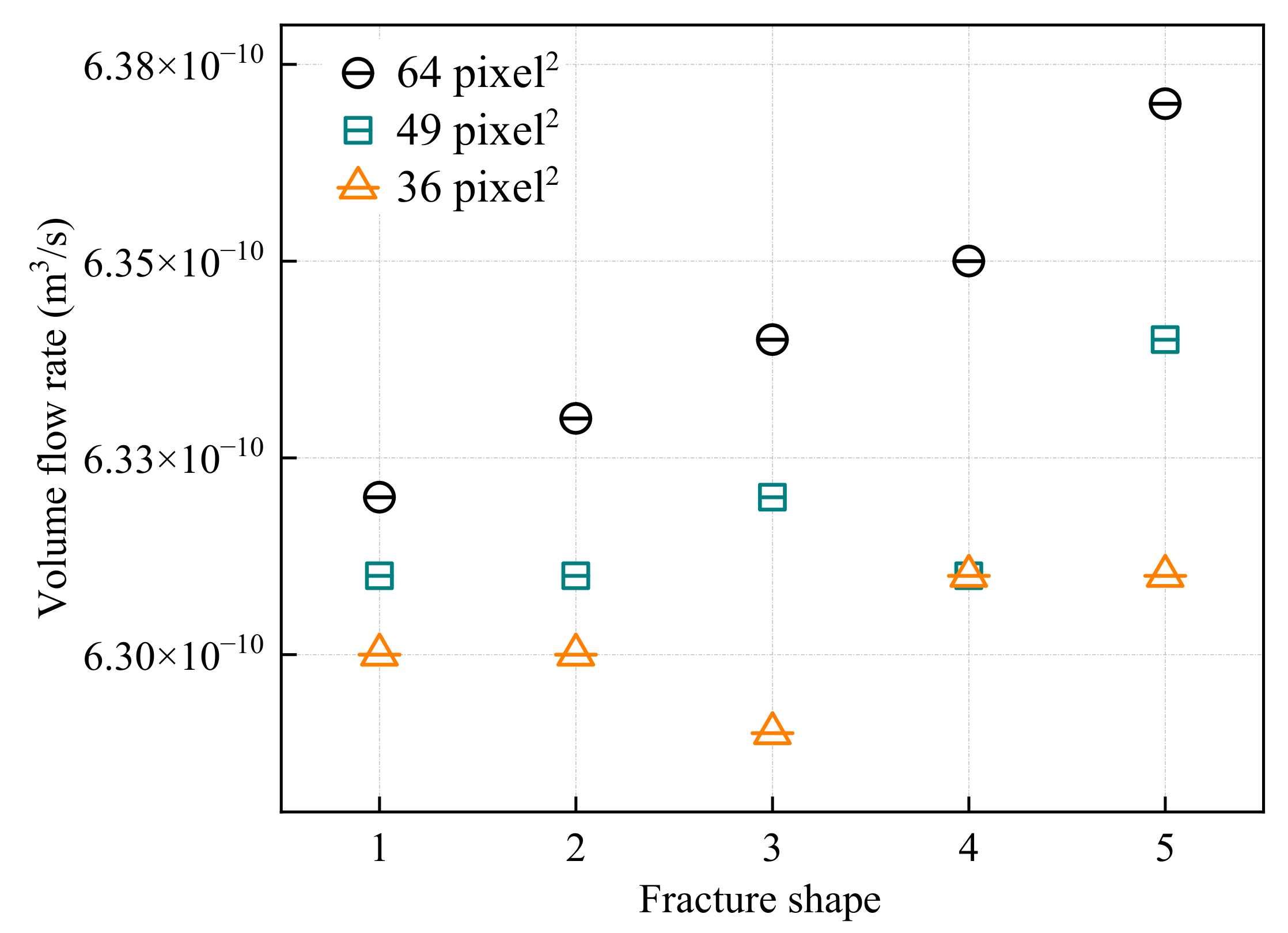
Applsci 12 04766 g013
Figure 14. Volume flow rate through a cement–rock sample: effect of variable microchannel shape and cross-sectional area.
Applsci 12 04766 g014
Figure 15. The velocity streamlines for cases with multiple microchannels and base case. (af): microchannel quantity = 1, 2, 3, 4, 5, 0 (base case).
Applsci 12 04766 g015
Figure 16. (a) Percentage of increase in the volume flow rate vs. number of microchannels, and (b) effect of increasing number of microchannels on the volume flow rate.
Applsci 12 04766 g016
Figure 17. The velocity streamlines for vertical and slanted microchannel cases: (a) circular 0°, (b) circular 13.89°, (c) circular 25.82°, (d) square 0°, (e) square 13.89°, (f) square 25.82°.
Applsci 12 04766 g017
Figure 18. (a) Contact area vs. inclination angle for slanted microchannel models with a 16 pixel2 (0.1279 mm2) circular microchannel and a 16 pixel2 (0.1279 mm2) square microchannel, respectively; (b) volume flow rate vs. contact area for slanted microchannel models with a 16 pixel2 (0.1279 mm2) circular microchannel and a 16 pixel2 (0.1279 mm2) square microchannel, respectively.
Applsci 12 04766 g018
Figure 19. The velocity streamlines for cases with different rock permeability. (ac): k1(krock < kinterface), k2 (krock = kinterface), k3 (krock > kinterface).
Applsci 12 04766 g019
Table 1. Mineral and chemical composition of the Notikewin rock [19].
PropertiesDetails
LithologyQuartzose sandy siltstone
Mineralogical compositionHigh amount of quartz with small amounts of dolomite, ankerite, muscovite, and albite
Major element composition (unit: ppm)Si (340136), Ca (33333), Al (31364), Fe (14598), K (9092), Mg (6883)
Table 2. Primary simulation parameters.
ParametersValues
Fluid flow regimeLaminar
Fluid typeWater at 25 °C
Domain type of the cement matrixPorous
Domain type of the rockPorous
Domain type of the interface Porous
Domain type of microchannelFluid
Porosity of the cement matrix0.011
Porosity of the rock matrix0.04
Porosity of the interface0.014
Permeability of the cement matrix9.86923 × 10−19 m2
Permeability of the rock6.908461 × 10−17 m2
Permeability of the interface4.9346 × 10−16 m2
Initial velocityU = 0, V = 0.1, W = 0 m/s
Max iterations1000
RMS residual level1 × 10−5
Boundary conditionTotal inlet pressure (stable) = 10 psi
Static outlet pressure (relative) = 0 psi
Table 3. Rock permeability values used for three cases of simulation studies.
CaseRock Permeability (m2)
k1 (krock < kinterface)6.908461 × 10⁻¹⁷
k2 (krock = kinterface)4.9346 × 10⁻¹⁶
k3 (krock > kinterface)1.70737 × 10⁻¹⁵
Table 4. Effect of micro channel shape on the volume flow rate through cement–rock sample: comparison of the base case (no microchannel) and case with 64 pixel2 (0.2273 mm2) microchannel.
SectionVolume Flow Rate (m3/s)
Base CaseCircle 64Oval 64Square 64Rectangle 64Triangle 64
Cement6.31 × 10−135.13 × 10−135.10 × 10−135.12 × 10−135.03 × 10−135.02 × 10⁻¹³
Interface2.19 × 10−101.82 × 10−101.80 × 10−101.81 × 10−101.79 × 10−101.78 × 10⁻¹⁰
Rock3.59 × 10−103.55 × 10−103.55 × 10−103.56 × 10−103.54 × 10−103.55 × 10⁻¹⁰
Microchannel/9.51 × 10−119.75 × 10−119.60 × 10−111.02 × 10−111.04 × 10⁻¹⁰
Total5.79 × 10−106.32 × 10−106.33 × 10−106.34 × 10−106.35 × 10−106.37 × 10⁻¹⁰
Percentage of increase/9.15%9.33%9.50%9.67%10.02%
Table 5. Effect of the microchannel contact area on the volume flow rate: data for cases with a 64 pixel2 (0.2273 mm2) microchannel.
CaseContact Area (m2)Volume Flow Rate (m3/s)Percentage Increase in Volume Flow Rate
Circle 641.02 × 10−56.32 × 10−109.15%
Oval 641.17 × 10−56.33 × 10−109.33%
Square 641.13 × 10−56.34 × 10−109.50%
Rectangle 641.43 × 10−56.35 × 10−109.67%
Triangle 641.60 × 10−56.37 × 10−1010.02%
Base Case/5.79 × 10−10/
Table 6. Volume flow rate through cement–rock sample: comparison of the base case (no microchannel) and microchannels with a 49 pixel2 (0.1741 mm2) cross-sectional area.
SectionVolume Flow Rate (m3/s)
Base CaseCircle 49Oval 49Square 49Rectangle 49Triangle 49
Cement6.31 × 10−135.15 × 10−135.11 × 10−135.15 × 10−135.12 × 10−135.09 × 10⁻¹³
Interface2.19 × 10−101.82 × 10−101.81 × 10−101.82 × 10−101.81 × 10−101.80 × 10⁻¹⁰
Rock3.59 × 10−103.55 × 10−103.53 × 10−103.55 × 10−103.53 × 10−103.55 × 10⁻¹⁰
Microchannel/9.36 × 10−119.58 × 10−119.40 × 10−119.54 × 10−119.77 × 10⁻¹¹
Total5.79 × 10−106.31 × 10−106.31 × 10−106.32 × 10−106.31 × 10−106.34 × 10⁻¹⁰
% of increase/8.98%8.98%9.15%8.98%9.50%
Table 7. Volume flow rate through cement–rock sample: comparison of the base case (no microchannel) and microchannels with a 36 pixel2 (0.1279 mm2) cross-sectional area.
SectionVolume Flow Rate (m3/s)
Base CaseCircle 36Oval 36Square 36Rectangle 36Triangle 36
Cement6.31 × 10−135.18 × 10−135.17 × 10−135.17 × 10−135.16 × 10−135.16 × 10⁻¹³
Interface2.19 × 10−101.83 × 10−101.83 × 10−101.83 × 10−101.83 × 10−101.83 × 10⁻¹⁰
Rock3.59 × 10−103.56 × 10−103.55 × 10−103.54 × 10−103.56 × 10−103.56 × 10⁻¹⁰
Microchannel/9.07 × 10−119.11 × 10−119.14 × 10−119.20 × 10−119.20 × 10⁻¹¹
Total5.79 × 10−106.30 × 10−106.30 × 10−106.29 × 10−106.31 × 10−106.31 × 10⁻¹⁰
% of increase/8.81%8.81%8.64%8.98%8.98%
Table 8. Volume flow rate through a cement–rock sample: effect of variable microchannel shape and the size of the cross-sectional area.
Microchannel ShapeVolume Flow Rate (m3/s)
0.2273 mm2 (64 Pixel2)0.1741 mm2 (49 Pixel2)0.1279 mm2 (36 Pixel2)
1. Circle6.32 × 10−106.31 × 10−106.30 × 10⁻¹⁰
2. Oval6.33 × 10−106.31 × 10−106.30 × 10⁻¹⁰
3. Square6.34 × 10−106.32 × 10−106.29 × 10⁻¹⁰
4. Rectangle6.35 × 10−106.31 × 10−106.31 × 10⁻¹⁰
5. Triangle6.37 × 10−106.34 × 10−106.31 × 10⁻¹⁰
Table 9. Contact area of microchannels with variable shape and cross-sectional area.
Microchannel ShapeContact Area (m2)
0.2273 mm2 (64 Pixel2)0.1741 mm2 (49 Pixel2)0.1279 mm2 (36 Pixel2)
1. Circle1.02 × 10−59.37 × 10−67.43 × 10−6
2. Oval1.17 × 10−51.05 × 10−57.77 × 10−6
3. Square1.13 × 10−59.73 × 10−68.19 × 10−6
4. Rectangle1.43 × 10−51.00 × 10−58.17 × 10−6
5. Triangle1.60 × 10−51.14 × 10−59.18 × 10−6
Table 10. Effects of the number of microchannels on the volume flow rate.
Number of MicrochannelsCross-Sectional Area (m2)Contact Area (m2)Total Volume Flow Rate (m3/s)Percentage of Increase
0005.79 × 10−10/
12.44 × 10−71.13 × 10−56.34 × 10−109.50%
24.92 × 10−72.25 × 10−56.85 × 10−1018.31%
37.41 × 10−73.37 × 10−57.32 × 10−1026.42%
49.85 × 10−74.51 × 10−57.65 × 10−1032.12%
51.27 × 10−65.91 × 10−57.89 × 10−1036.27%
Table 11. Volume flow rate and contact area of slanted microchannels with circular shape.
CaseInclination Angle, α (Degree)Volume Flow Rate (m3/s)Cross-Sectional Area (m2)Contact Area (m2)
Circle-i225.826.29 × 10−103.22 × 10−84.40 × 10−6
Circle-i413.896.28 × 10−103.20 × 10−84.33 × 10−6
Base case06.25 × 10−103.18 × 10−84.31 × 10−6
Table 12. Volume flow rate and contact area of slanted microchannels with square shape.
CaseInclination Angle, α (Degree)Volume Flow Rate (m3/s)Cross-Sectional Area (m2)Contact Area (m2)
Square-i225.826.30 × 10−104.84 × 10−85.28 × 10−6
Square-i413.896.29 × 10−104.64 × 10−85.18 × 10−6
Base case06.28 × 10−104.84 × 10−85.12 × 10−6
Table 13. Volume flow rate through cement–rock samples with microchannels and variable rock permeability.
SectionVolume Flow Rate (m3/s)
k1 (Krock < Kinterface)k2 (Krock = Kinterface)k3 (Krock > Kinterface)
Cement5.12 × 10−139.02 × 10−131.02 × 10⁻¹²
Interface1.81 × 10−103.50 × 10−104.13 × 10⁻¹⁰
Rock3.56 × 10−102.73 × 10−99.70 × 10−9
Microchannel9.60 × 10−113.28 × 10−105.75 × 10⁻¹⁰
Total6.34 × 10−103.41 × 10−91.07 × 10−8
Table 14. Average outflow velocity through a cement–rock sample with microchannels and variable rock permeability.
SectionAverage Outflow Velocity (m/s)
k1 (Krock < Kinterface)k2 (Krock = Kinterface)k3 (Krock > Kinterface)
Cement1.19 × 10−82.11 × 10−82.39 × 10−8
Interface7.72 × 10−61.49 × 10−51.76 × 10−5
Rock6.32 × 10−64.84 × 10−51.72 × 10−4
Microchannel3.94 × 10−41.35 × 10−32.36 × 10−3
Total5.16 × 10−62.77 × 10−58.70 × 10−5
Publisher’s Note: MDPI stays neutral with regard to jurisdictional claims in published maps and institutional affiliations.

