Article

The Propagation of Hydraulic Fractures in a Natural Fracture Network: A Numerical Study and Its Implications

1
School of Civil and Architectural Engineering, Wuhan University, Wuhan 430072, China
2
Hubei Key Laboratory of Waterjet Theory and New Technology, Wuhan University, Wuhan 430072, China
3
The Institute of Technological Sciences, Wuhan University, Wuhan 430072, China
4
School of Power and Mechanical Engineering, Wuhan University, Wuhan 430072, China
*
Author to whom correspondence should be addressed.
Appl. Sci. 2022, 12(9), 4738; https://doi.org/10.3390/app12094738
Submission received: 28 March 2022 / Revised: 30 April 2022 / Accepted: 4 May 2022 / Published: 8 May 2022
(This article belongs to the Special Issue Geomechanics and Reservoirs: Modeling and Simulation)

Abstract

:
Natural fractures play a significant role in creating a fracture network simulation treatment. In this work, global cohesive elements were incorporated into the cohesive zone method to realize the unprompted propagation of a hydraulic fracture. The step-by-step propagation patterns of hydraulic fractures in a random natural fracture network were discussed. An effective area was defined to quantitively assess the influenced area of induced fractures. The results showed that the hydraulic fracture tips were attracted by local natural fractures when the horizontal stress difference was low. Bifurcations and secondary fractures occurred at the natural fracture intersections, which contributed to the complexity of the induced fracture network on a local scale. The length of the main hydraulic fracture reached the maximum when the in situ stress ratio was 1.12. The influence of natural fractures on the overall trend of fracture propagation was limited when the in situ stress difference increased. It also suggested that a lower rock tensile strength and natural fractures cementation strength improved the main fracture length. A higher tensile strength of rock increased the initiation pressure of the induced fracture, while the cementing strength of the natural fractures showed no impact on it. The results presented in this paper could improve the basic understanding of the fracture development in a natural network and help to predict a complex fracture network in a real situation.

1. Introduction

The successful and efficient exploitation of shale gas heavily relies on hydraulic fracturing to achieve commercial production [1], which is the most effective way to recover the gas from low permeability naturally fractured formations [2]. Creating a complex fracture network system is the most important goal of hydraulic fracturing in ultra-low permeability reservoirs. However, geological materials are discontinuous and heterogeneous due to the tectonic action of strata. Discontinuous joints and natural fractures that are randomly distributed in the reservoirs have a significant influence on the fracture network geometries. Observations of core samples and image logging indicates that discontinuities in shale, such as natural fractures and bedding interfaces, exist in most shale reservoirs and act as weak planes to affect the propagation of hydraulic fracture [3]. Field fracturing tests and microseismic monitoring reveal that hydro-induced fractures in hydraulic fracturing can activate natural fractures and weak planes in the reservoir, thus generating a large number of branch fractures, and significantly improving the permeability of the reservoir [4,5,6].
In the past decades, many studies have been conducted to investigate the effects of discontinuities (e.g., natural fractures and joints) on perturbing the propagation of hydraulic fractures, and the results reveal that natural fractures can observably improve the ultimate morphology of the fracture network [7,8,9]. For instance, Maxwell and Steinsberger [10] used microseismic monitoring technology to image hydraulic fracturing fractures in shale, revealing a positive correlation between gas production and fracture network complexity. Renshaw and Pollard [11] established an orthogonal intersection criterion of hydraulic fractures and natural fractures to predict whether the hydrofractures in brittle rocks would propagate through natural fractures or terminate after they intersected vertically. Later, Gu [12] supplemented the orthogonal intersection criterion and found that a hydraulic fracture was more likely to extend along the interface of a natural fracture when their intersection angle was less than 90°, which has been verified by experiments. Bahorich [13] reported that there might be bypass, separation of weak planes, fracture deflection, and mixed expansion of the above three modes at the intersection of hydraulic fractures and natural fractures. They concluded that the presence of these natural fractures can have beneficial or detrimental effects on the complex geometry of hydrofractures. On the one hand, the activation of natural fractures may expand the flow paths of oil and gas and improve fracture complexity, making stimulation treatments more effective [14]. On the other hand, reactivated natural fractures may result in additional leak-off and reduced fluid pressure in fractures, hence a lower treatment fluid efficiency [15]. Despite the existing research results, most experiments or numerical model have been devoted to investigating the interaction of a single natural fracture or several hydraulic fractures but ignore the natural fractures in the form of a network. A thorough understanding of the fracture propagation behavior in a natural fracture network is still lacking.
In recent years, some studies have focused on large-scale fracture network simulation. New hydraulic fracturing models have been developed and are still evolving. So far, the main methods used to simulate complex fracture networks are the Displacement Discontinuous Method (DDM) [16,17,18,19], Boundary Element Method (BEM) [20], Finite Element Method (FEM) [21,22], Extended Finite Element Method (XFEM) [23,24], Discrete Fracture Network (DFN) [25,26,27], and the Discrete Element Method (DEM) [28,29]. Each of these methods has advantages and disadvantages: the DDM has some difficulties in the deformation of heterogeneous and anisotropic materials; the DEM has a high computing cost in the computing domain; the FEM is an effective and widely used numerical technique, but it is time consuming due to grid repartition. The Cohesive Zone Method (CZM), an efficient tool for fracture initiation and propagation modeling that has been developed in recent years, can help to solve these problems [30,31,32,33]. In the CZM, cohesive elements with pore pressure DOF and displacement DOF are used to describe hydrofractures with consideration of fluid flow in the fracture and leak-off to the rock [34,35], as shown in Figure 1. The fracture process is characterized by the Traction-Separation Law, which mainly depends on the material properties of the cohesive zone. The CZM successfully circumvents the significant perturbance that the singularity at the fracture tip causes in the solution convergence of the equations. In addition, the CZM imposes restrictions on the hydraulic fractures’ propagation paths and only allows fractures to extend along the edges of cohesive elements. Hence, the FEM in conjunction with the cohesive layer can explicitly model the simulation of the intersection between hydraulic fractures and natural fractures without grid remeshing, which reduces the computational expense [36]. However, this propagation restriction is also the main shortcoming of CZM. It requires that the direction of the propagation of the fracture must be known or actively updated during propagation. In other words, the intersection at a natural fracture is predefined and not predicted. Three types of interactions are observed between a hydraulic and a single natural fracture [15], in which we can preset the expansion path of fractures, but this cannot be achieved in the natural fracture network due to the much more complicated fracture geometries. A key consideration of a complex fracture model is the propagation of a hydraulic fracture in a connective natural fracture network. In this case, fracture propagation may occur along the reactivated natural fracture paths with complex geometries, including deflections and bifurcations. In this way, the intersection mechanism between the fracture and the single natural fracture is not so important, but the influence of the fracture network should be considered.
In field tests or experimental tests, the development process of induced fractures in rocks is actually unknown, making it hard to understand the role that natural fractures play in induced fracture propagation. In this paper, we investigated the step-by-step propagation pattern of hydraulic fractures in a natural fracture network and realized the non-prefabricated propagation of hydraulic fractures by using global cohesive elements. The effects of multiple factors such as in situ horizontal stress, rock tensile strength, and natural fracture cementation strength were discussed. The results presented in this paper could provide a visible propagation process of a hydraulic fracture and improve the basic understanding of the fracture development in a natural network. It helps the prediction of a complex fracture network in a real situation.

2. Simulation Methodology

2.1. Coupled Pore Fluid Diffusion and Stress Analysis

Fracture propagation behavior of hydraulic fracturing is a fluid–solid coupling problem, concerned with the deformation of the solid phase, fluid flow in the porous media, fracturing fluid flow in the fracture, and fracturing fluid leak-off. In this paper, coupled pore fluid diffusion and stress analysis were used to simulate the propagation of a hydrofracture in rock. The rock was regarded as a multiphase material, and an effective stress principle was adopted to describe its behavior. When the pores in the porous medium are filled with single-phase liquid medium, the effective stress of the porous medium is defined as follow:
σ ¯ * = σ + χ u w I
where σ ¯ * is effective stress, σ is total stress, and χ is a factor that depends on saturation and surface tension of the liquid-solid system [37]; it is 1.0 when the medium is fully saturated. u w is the fluid pressure of the porous medium, and I is the second-order tensor.
The rock stress equilibrium equation can be expressed by the principle of virtual work as follow:
V σ · δ ε d V S t · δ v d S V f · δ v d V = 0
where δ v is the virtual velocity field, δ ε is the virtual deformation, σ is the Cauchy stress, t is the surface traction of per unit area, and f is the body force of per unit volume.
We considered the presence of liquid fluids in porous medium and assumed that the fluid was relatively incompressible. The porous medium was modeled by attaching finite element mesh to solid phase, and a continuity equation was used to calculate the mass of liquid in unit volume of porous media, which was written in a variational form as a basis for finite element approximation. The total mass of the liquid in volume (occupies space V with surface S) can be written as:
V ρ w [ d V w + d V t ] = V ρ w ( n w + n t ) d V
where ρ w is the mass density of the liquid, V w is the volume of liquid that passes through at any time, and V t is the volume of liquid trapped at any time. The time rate of change in this mass of liquid can be calculated as:
d d t ( V ρ w ( n w + n t ) d V ) = V 1 J d d t ( J ρ w ( n w + n t ) ) d V
where J is the volume change in the material. The mass of the liquid passing through the surface into the volume in unit time is:
S ρ w n w n · v w d S
where v w is the average velocity of the liquid relative to the solid phase (seepage velocity), and n is the outward normal of S. The mass continuity equation of wetting liquid is obtained by equating the increase in liquid mass on surface S to the change rate in liquid mass in volume V as follows:
V 1 J d d t ( J ρ w ( n w + n t ) ) d V = S ρ w n w n · v w d S
Equation (6) is integrated approximately in time by the backward Euler formula and introducing Darcy’s law to describe the constitutive behavior of pore fluid; then, the continuity statement for the liquid phase in a porous medium can be obtained:
V [ δ u w ( ρ w ρ w 0 ( n w + n t ) 1 J ( ρ w ρ w 0 ( J ( n w + n t ) ) t ) Δ t k s ρ w 0 g ( 1 + β v w · v w ) δ u w x · k · ( u w x ρ w g ) ] d V + Δ t S δ u w ρ w ρ w 0 n w n · v w d S = 0
where δ u w is an arbitrary continuous variational field, β is the velocity coefficient [38], k is the permeability of the saturated medium, and g is the gravitational acceleration. The equation was normalized by the density of the liquid in the reference configuration for convenience, ρ w 0 .
In a coupled procedure, Equations (1), (2), and (7) are collated into a matrix expression, and the simultaneous solution can be used to derive the fluid–solid coupling finite element equation of the reservoir. Newton iterations are used to solve the equation.

2.2. Fracture Initiation and Propagation Criteria

Various criteria have been proposed to predict fracture initiation and propagation [39,40,41,42], mainly based on linear elastic fracture mechanics (LEFM) theory and damage mechanics. The LEFM method uses characteristic parameters such as the stress intensity factor and energy release rate as criteria for fracture propagation judgement. The LEFM is unable to predict the fracture initiation and is typically used to predict the propagation of cracks that have been opened in the material. Another major method of crack prediction is based on damage mechanics, in which the microdefects inside the material are considered. By selecting appropriate damage variables, the damage evolution equation of the damage-containing materials is derived using continuum mechanics [43,44,45].
In this paper, a linear Traction-Separation Law based on damage mechanics is used to judge the crack propagation behavior. It assumes that the failure of the cohesive elements is characterized by the progressive degradation of the material stiffness, which is driven by a damage process. The failure mechanism consists of two ingredients: a damage initiation criterion and a damage evolution law.
The stress and strain follow the linear elastic relationship before the damage occurs in a cohesive element. Traction t = { t n , t s , t t } , where t n is the traction perpendicular to the possible fracture surface, and t s , t t are two tangential tractions perpendicular to each other on possible fracture surfaces. t n 0 , t s 0 , and t t 0 represent the limit values of nominal stress, respectively. Once any component of the traction reaches the limit value, the cohesive element begins to be damaged, and the fracture occurs. This damage initiation criteria can be expressed as [46]:
max { t n t n 0 , t s t s 0 , t t t t 0 } = 1
where the symbol   denotes the Macaulay bracket and signifies that a pure compressive deformation or stress state does not initiate damage.
With the injection of fracturing fluid, the traction increases as the fracture surface separates from each other. With the increase in separation degree, due to the degradation (or softening behavior) of the stiffness of the material, the traction decreases [47] until the fracture tip is completely destroyed, and the tractive strength of the fracture surface drops to zero. The damage evolution law can be characterized by a bilinear cohesion traction-separation relationship [48], shown in Figure 2, which can be expressed as follows:
t = { K 0 Δ   ,                               0 Δ Δ 0 ( 1 D ) K 0 Δ ,             Δ 0 Δ Δ m a x 0 ,                                     Δ m a x Δ
where K 0 is the initial stiffness of the cohesive element, Δ 0 is the critical displacement at which the fracture tip begins to damage, Δ m a x is the maximum displacement obtained during the loading process, and the damage index D is used to describe the damage degree of the cohesive element.

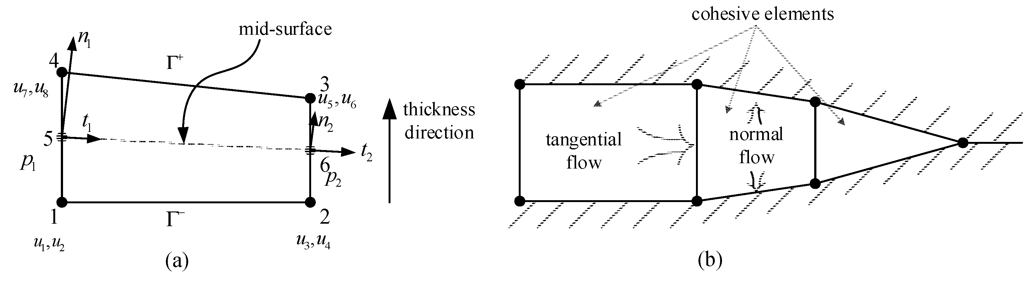
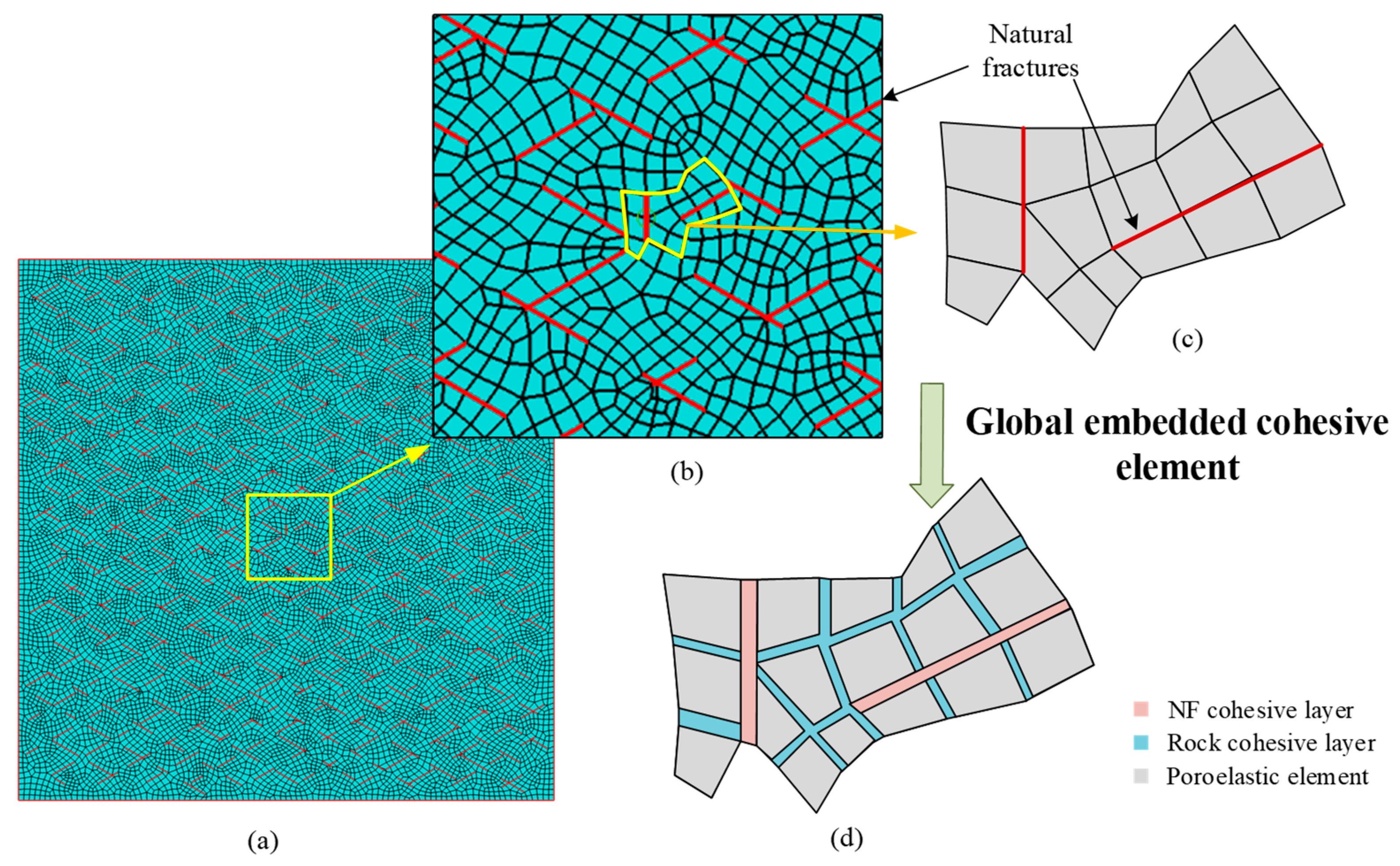
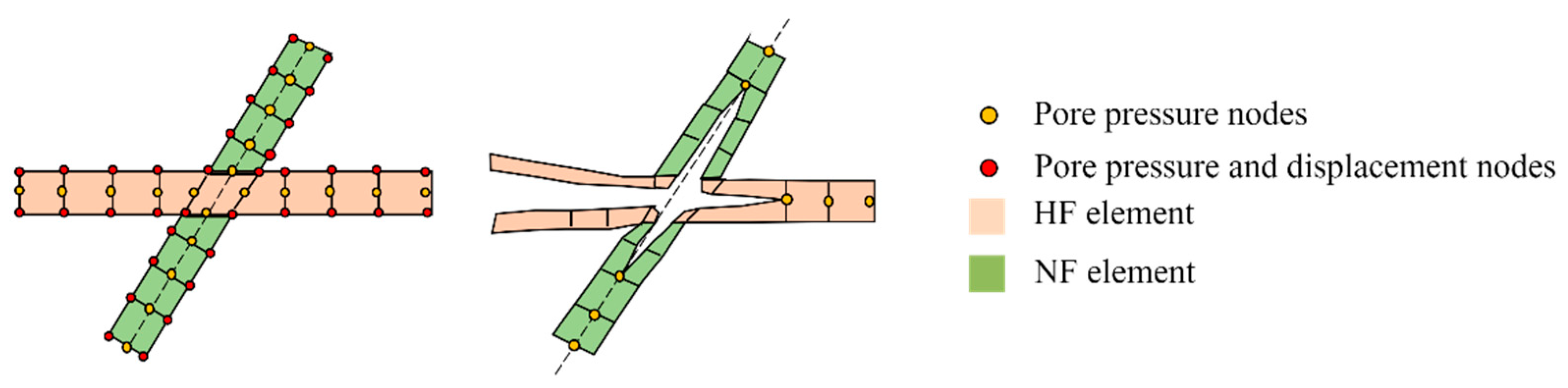
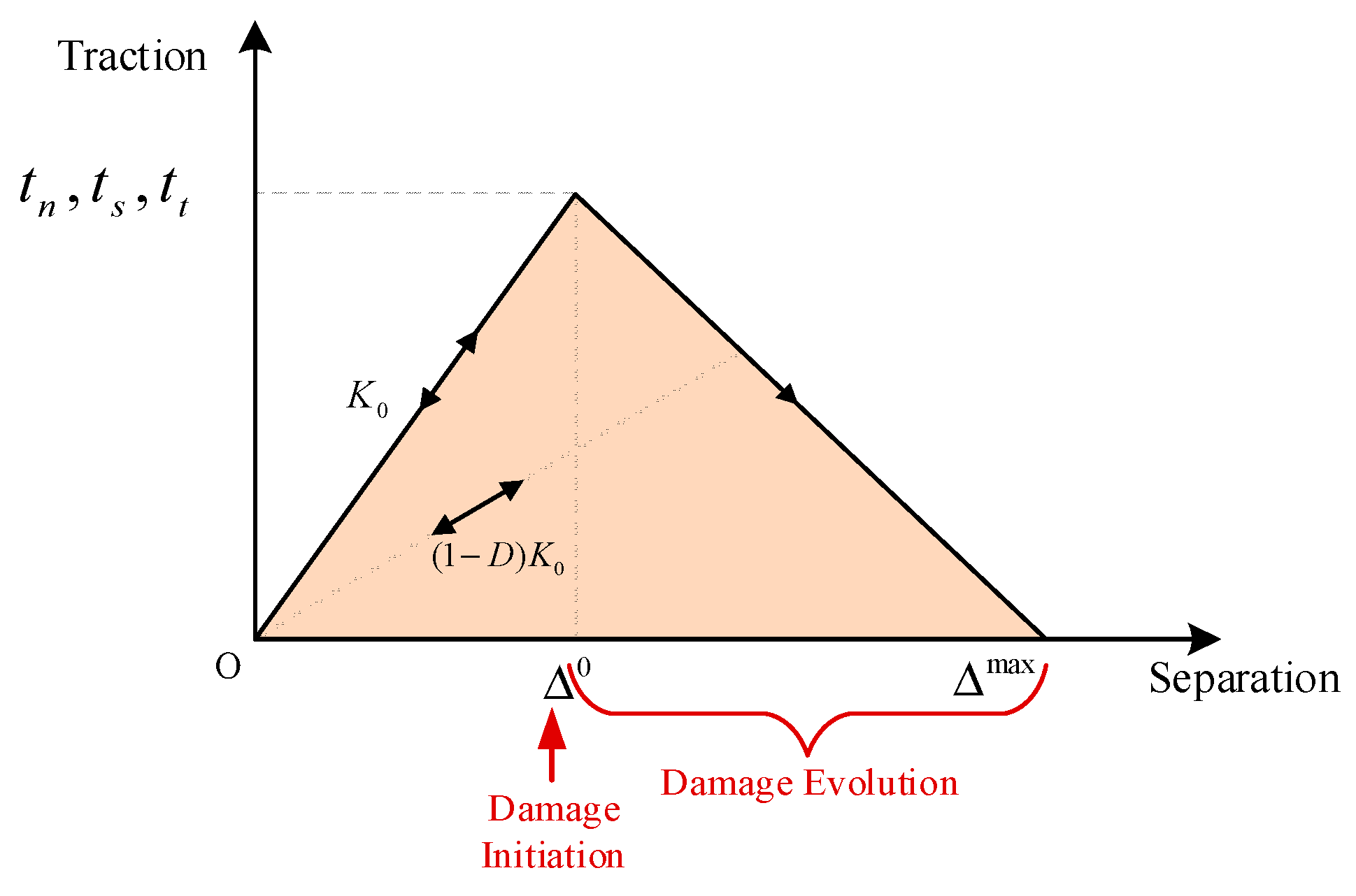
2.3. Global Cohesive Element Model

Generally, cohesive elements are considered as being composed of two faces separated by a thickness, as depicted in Figure 3a. The relative motion of the bottom and top faces measured along the thickness direction represents the opening and closing of fractures. The relative change in position of the bottom and top faces measured in the plane orthogonal to the thickness direction quantifies the transverse shear behavior of the cohesive element. The bottom surface and the top surface of the element will internally form intermediate pore pressure nodes, which can be observed in Figure 3a (node 5 and node 6). When the mid-surface is separated, driven by the fluid pressure, the fracturing fluid fills the fracture space; then, as shown in Figure 3b, normal flow occurs towards the top and bottom surface while tangential flow takes place at the intermediate node. In the CZM, the fractures are restricted to propagate along the cohesive element layer without being deflected into the rock matrix, as shown in Figure 4, which requires how the fracture will propagate be known. However, it is quite difficult to prefabricate all the fracture propagation paths in a naturally fractured formation, as fully developed natural fractures will greatly increase the morphology complexity of hydraulic fractures. In this work, we realize the fracture to extend along any element boundary after it initiates by using global cohesive elements. The cohesive element COH2D4P with pore pressure DOF was inserted arbitrarily into two adjacent rock elements and a natural fracture element. The cohesive elements were zero geometric thickness, which guaranteed the mechanical properties of the rock would not be affected. Since the fluid pressure is transmitted through intermediate pore pressure nodes, pore pressure nodes are shared between any two adjacent elements by converging all the intermediate nodes together, as schematically shown in Figure 5.

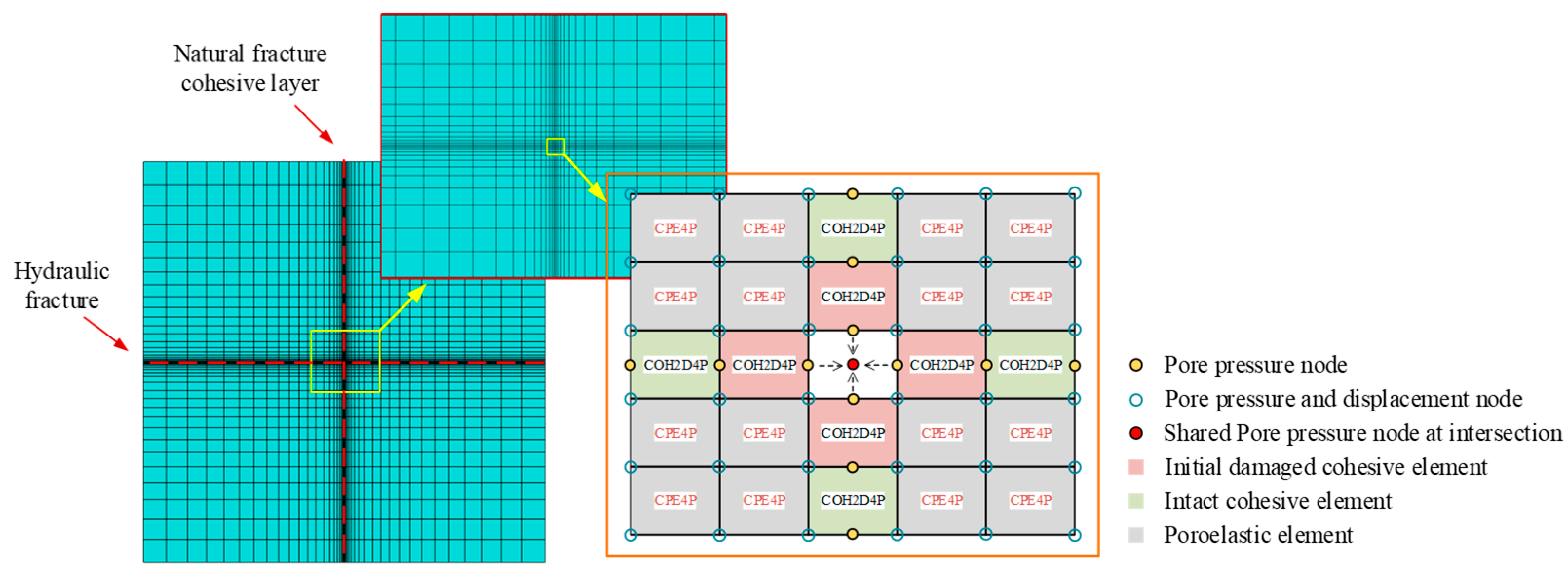
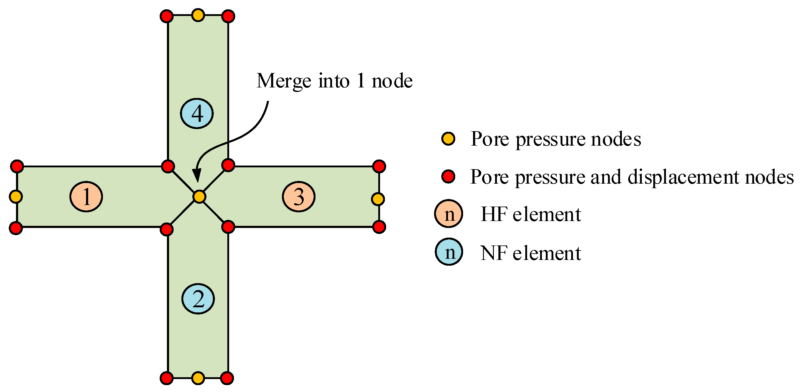
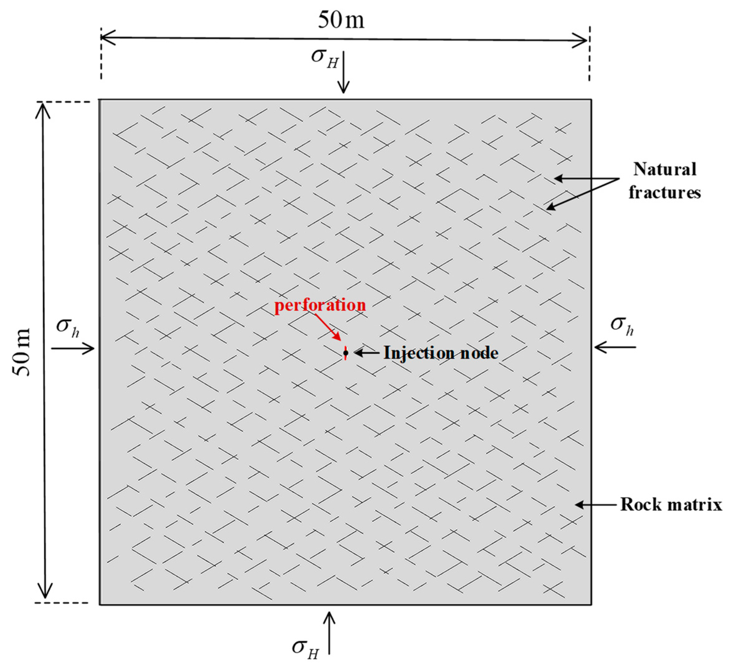
3. Complex Natural Global Cohesive Element Model Setup

The model size was 50 m × 50 m, with uniformly distributed in situ stress loaded on the boundary, as depicted in Figure 6. The maximum in situ horizontal stress σ H was in the vertical direction, and the minimum in situ horizontal stress σ h was in the horizontal direction. A 1-m-long perforation was prefabricated at the center of the model with an injection node at the midpoint. Fracturing fluid entered the model from the injection node and flowed through the perforation. About five hundred natural fractures were randomly distributed in two symmetrical directions with certain restrictions as follows: (1) the fracture length was in a specified range (1 m, 3 m); (2) the fracture length spacing range was (1 m, 2 m); (3) the fracture width spacing range was (2 m, 3 m); and (4) the x coordinate of the starting point was half length of the model diagonal to ensure that the natural fracture network center was at the center of the model. The natural fracture network model was programmed in Python, and the Newton-Raphson algorithm was used to analyze the diffusion and stress of the coupling pore fluid in the model. Modelling the initiation and propagation of hydraulic fracture intersecting with natural fractures network is a strongly nonlinear problem, involving the multi-field coupling effect of stress field and seepage; so, a powerful solver is needed. The calculation process was implemented in the finite element commercial software ABAQUS. Figure 7 shows the principle of the global cohesive element model. Two steps were included in the coupled pore fluid diffusion and stress analysis: (1) a geostatic step, which established equilibrium between the initial pore pressure and in situ stresses and removed the initial deformation; (2) a soil step, which simulated the hydraulic fracture initiation and propagation under the coupling of the rock skeleton and pore fluid. Natural fractures were assumed to be closed as the weak planes and assigned relatively smaller rock mechanical parameters, until driven by the fluid pressure under the Traction-Separation Law.
In order to make the simulation results more valuable for field tests, the model parameters referred to the real parameters of the Jiaoye No. 1 well in the Wufeng-Longmaxi Formation in Fuling, Sichuan Province, China [49]. The formation geologic parameters and material properties are listed in Table 1.

4. Numerical Results and Discussion

In this section, the previously built model is used to investigate the hydraulic fracture propagation in natural fracture network under multiple factors such as in situ horizontal stress, rock tensile strength, and natural fracture cementation strength.

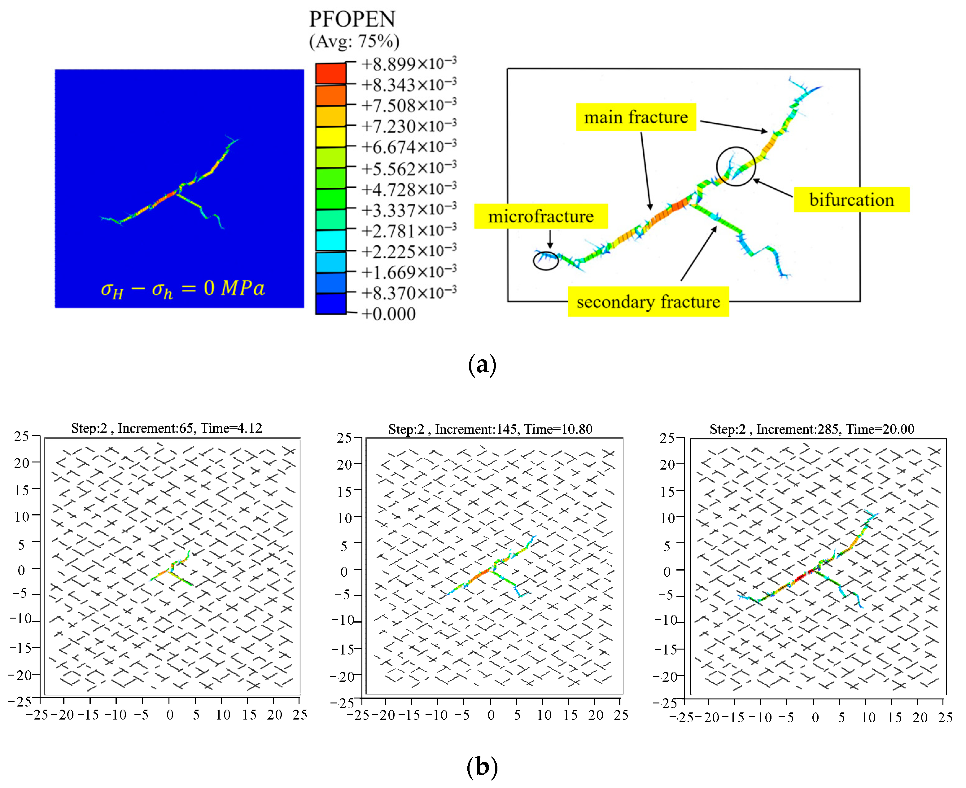
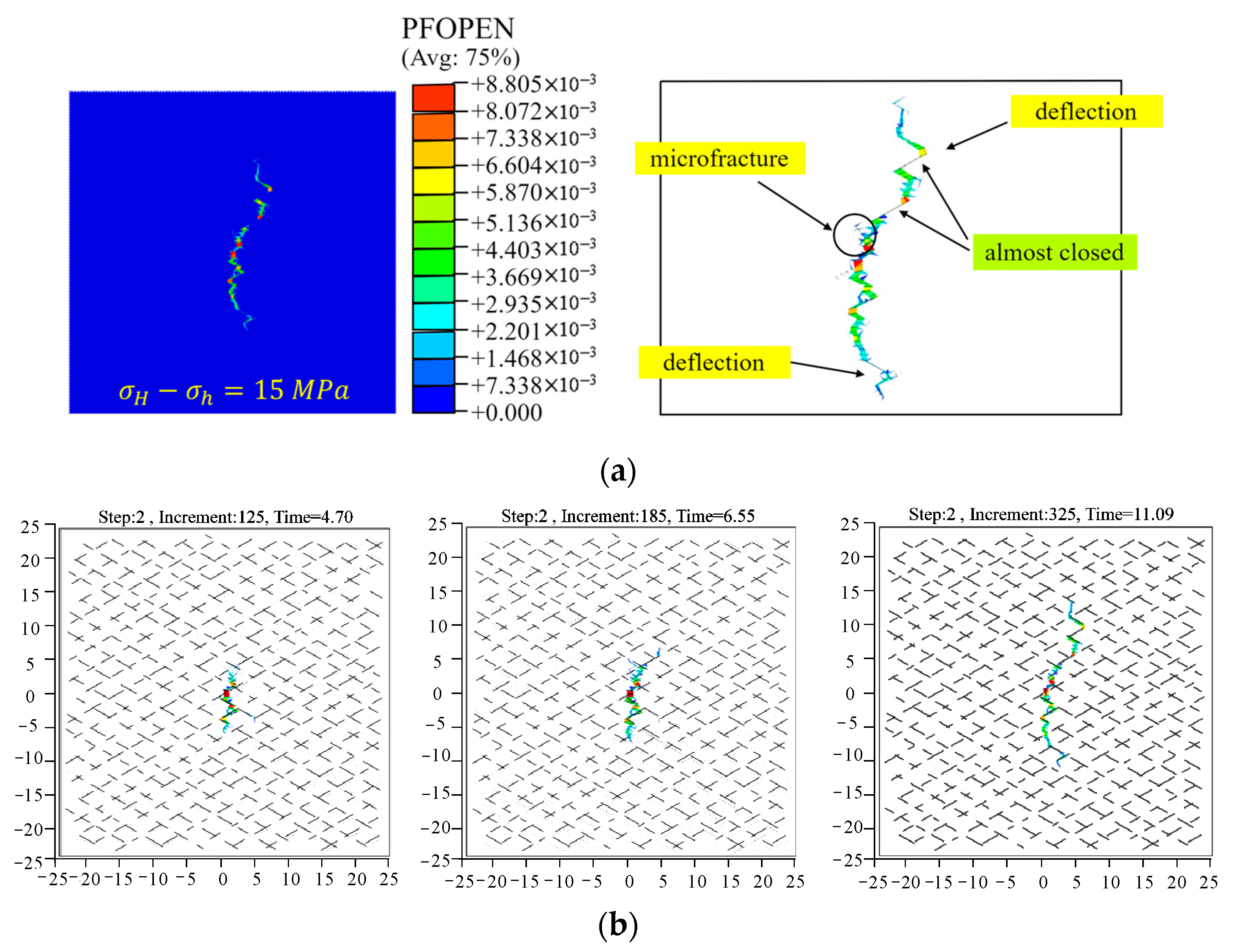
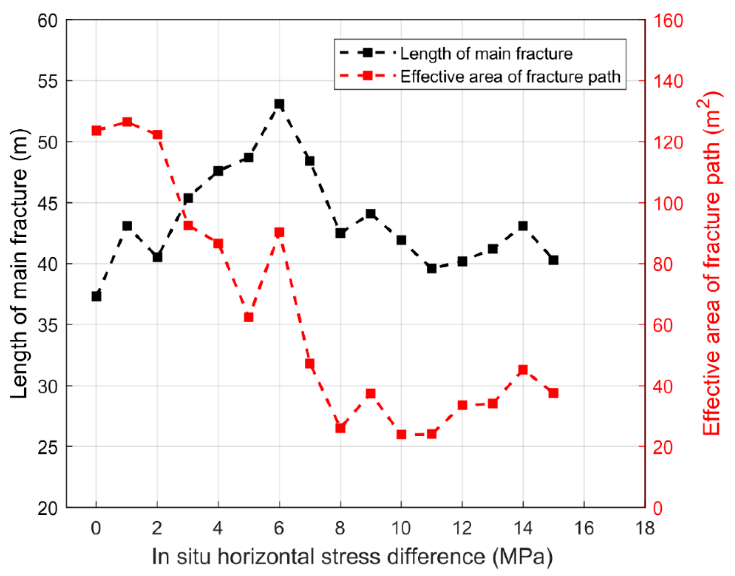
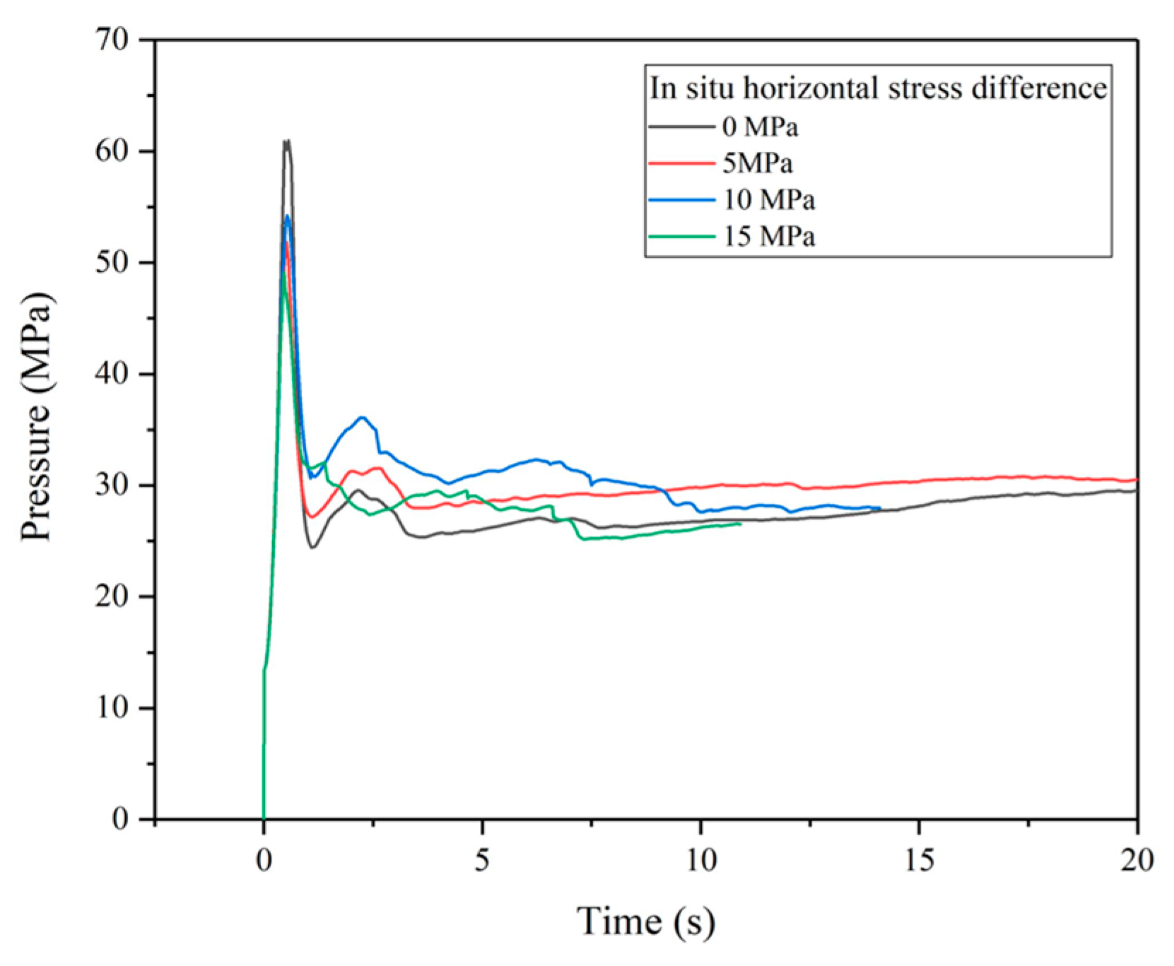
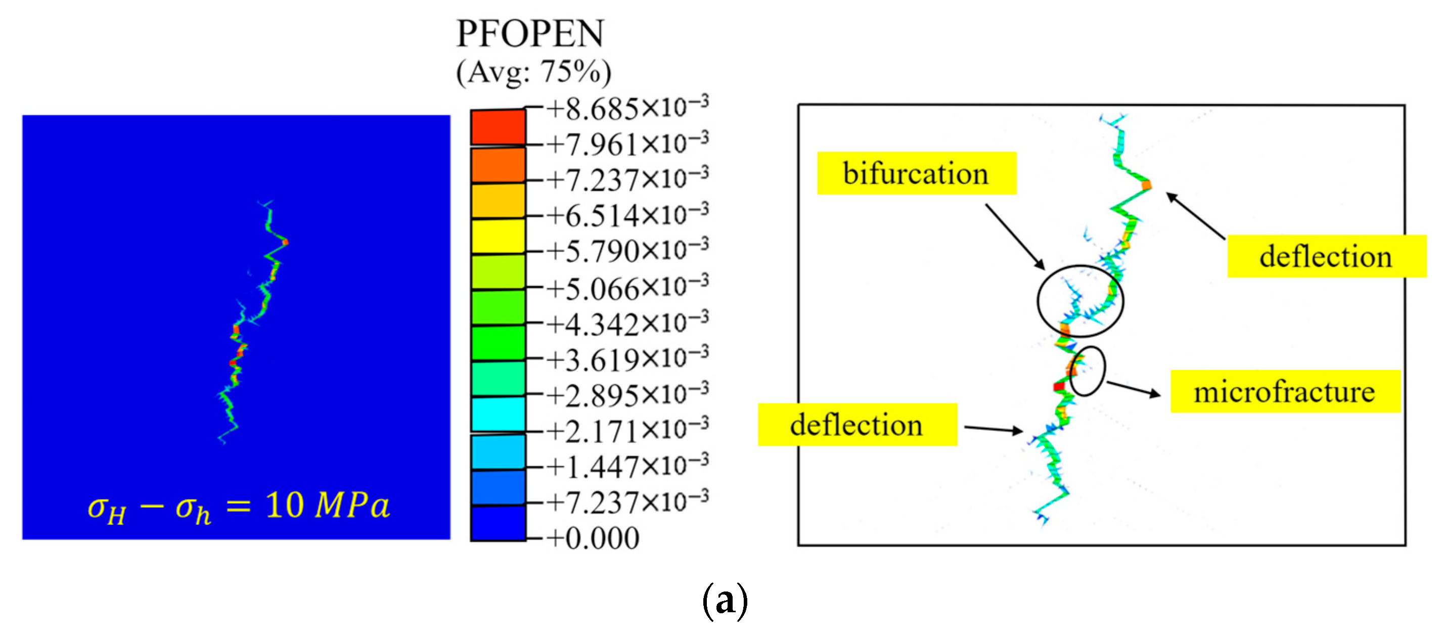
4.1. Influence of In situ Stress

To investigate the influence of in situ stress on hydraulic fracture propagation, we kept the minimum in situ stress at 50 MPa, while the maximum in situ horizontal stress ranged from 50 MPa to 65 MPa. The acute angle of the natural fracture and the maximum in situ horizontal stress was assigned to be 60°.
The simulation results are presented in Figure 8, Figure 9, Figure 10, Figure 11 and Figure 12, which indicate that the in situ horizontal stress difference played a critical role in the propagation of hydrofractures in a natural fracture network. Figure 8 shows the extracted hydraulic fractures’ morphology under different in situ stress differences. It is observed that under a small in situ stress difference, the induced fracture propagated at an angle with the horizontal stress direction and developed secondary fractures. With the increase in in situ stress differences, the angle of the induced fracture with maximum in situ horizontal stress became smaller, and no more secondary fractures occurred.
To understand the propagation pattern of the hydraulic fractures, we analyzed the step-by-step fracture development when the in situ stress differences were 0 MPa, 5 MPa, 10 MPa, and 15 MPa, as shown in Figure 9, Figure 10, Figure 11 and Figure 12. When the horizontal in situ stress difference was 0 MPa, the hydrofracture in the natural fracture network was no longer a symmetrical bi-wing fracture but complicated and tortuous. It initiated at the ends of the perforation, then expanded along the right-hand natural fractures, and finally formed a main fracture at about 60° to the vertical. After the main fracture above the perforation developed for a short distance, a bifurcation occurred and, then, stopped cracking quickly. The other branch at the bifurcation continued to propagate in the direction of the right-sloping natural fractures and turned to the 45° slowly. When it came to the fracture below the perforation, a secondary fracture appeared in the direction of the left-sloping natural fractures with several obvious turns during the propagation. In addition, burry-like microfractures were observed on the edges of major fractures.
To figure out the mechanism of fracture propagation in a natural fracture network, we extracted the coordinates of natural cracks and hydraulic fractures at different times, as depicted in Figure 9b. The 0 MPa in situ stress difference means that there was no preferential direction. As weak planes in the rock, the location of natural fractures might observably attract the hydrofracture. Thus, the induced fracture propagated along the nearest right-sloping natural fractures after it initiated, since they were closer than the left-sloping ones. Thereafter, the fracture tip continuously captured the nearest weak plane to extend. At the intersection of natural fractures in different directions, the two natural fractures may be reactivated simultaneously, where fracturing fluid distributed and lead to bifurcation and secondary fracture.
When the in situ stress difference was 5 MPa, a tortuous hydraulic fracture was formed with no secondary fracture, as illustrated in Figure 9. Influenced by the difference in in situ stress, the main fracture propagated along the right-sloping natural fractures at the outset but later deviated toward the direction of maximum in situ horizontal stress. It seems that the attraction of weak planes did not play a dominant role all the time. Several deflections occurred in the later process of the propagation. Unlike the result when the in situ stress difference was 0 MPa, the hydraulic fracture directly turned to the rock matrix under the in situ stress difference rather than go on along another natural fracture at the intersection.
The deviation of the hydraulic fracture from the direction of natural fractures was more obvious when the in situ stress difference was 10 MPa and 15 MPa. The hydraulic fracture initiated from the perforation and, distinctively, was not affected by the natural fracture near the perforation and propagated towards the direction of the maximum horizontal stress. The hydrofracture below the perforation was substantially in the vertical direction in its propagation and turned to the direction of the maximum horizontal principal stress immediately after it was captured and penetrated by natural fractures. The hydrofracture above the perforation first propagated in the vertical direction and, then, turned to the adjacent natural fractures and penetrated out along a zigzag. The overall trend of the hydraulic fracture no longer followed the direction of the natural fractures and propagated almost parallel to the direction of the maximum principal stress in twists and turns because of the large in situ stress difference. The attraction of weak planes was diminished. Although the position of natural fractures had limited influence on the overall trend of fracture propagation, it increased the sinuosity of the fracture morphology.

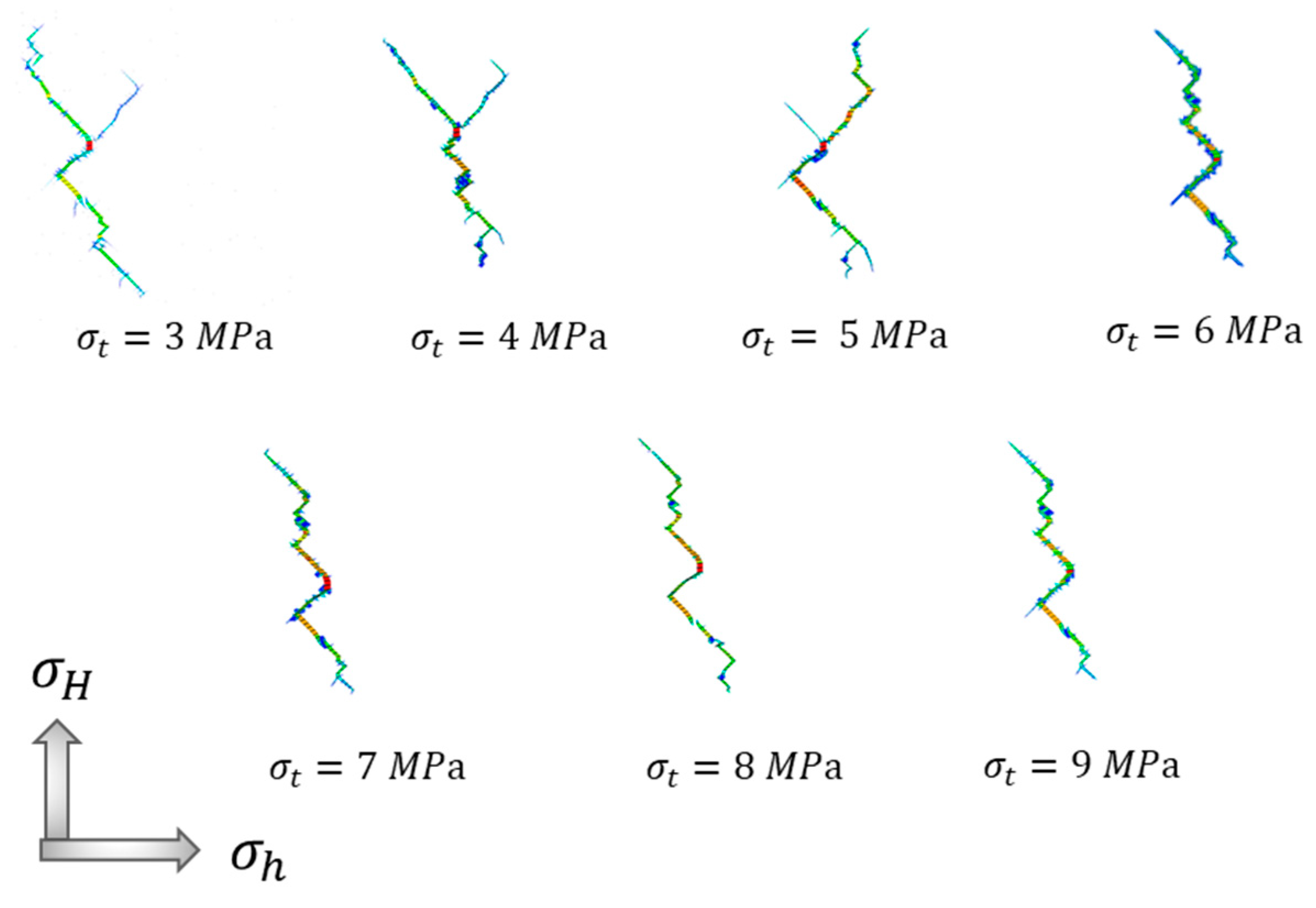
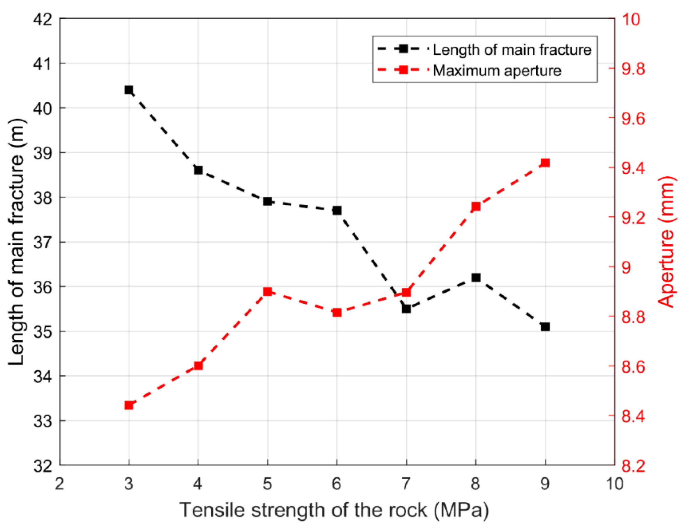
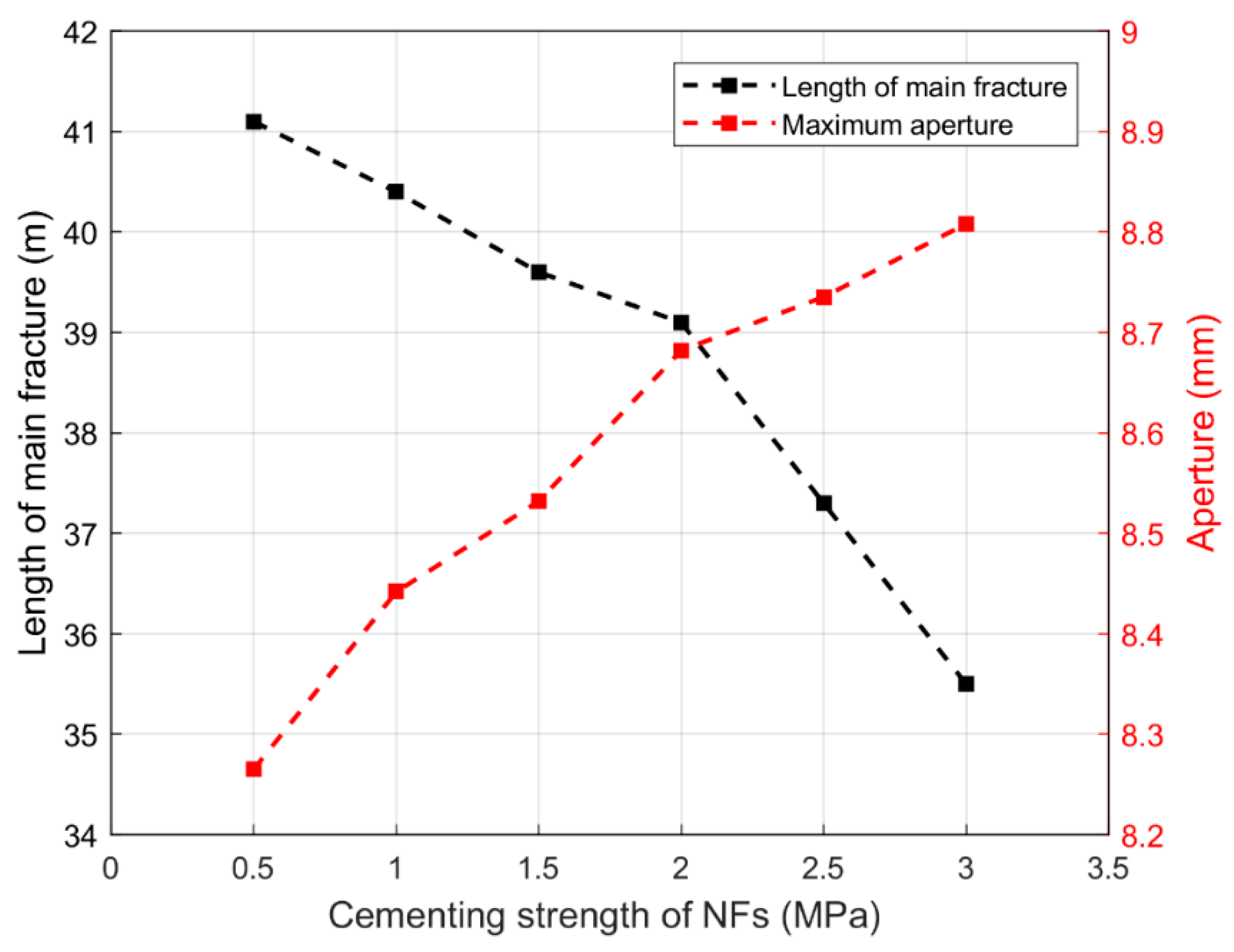
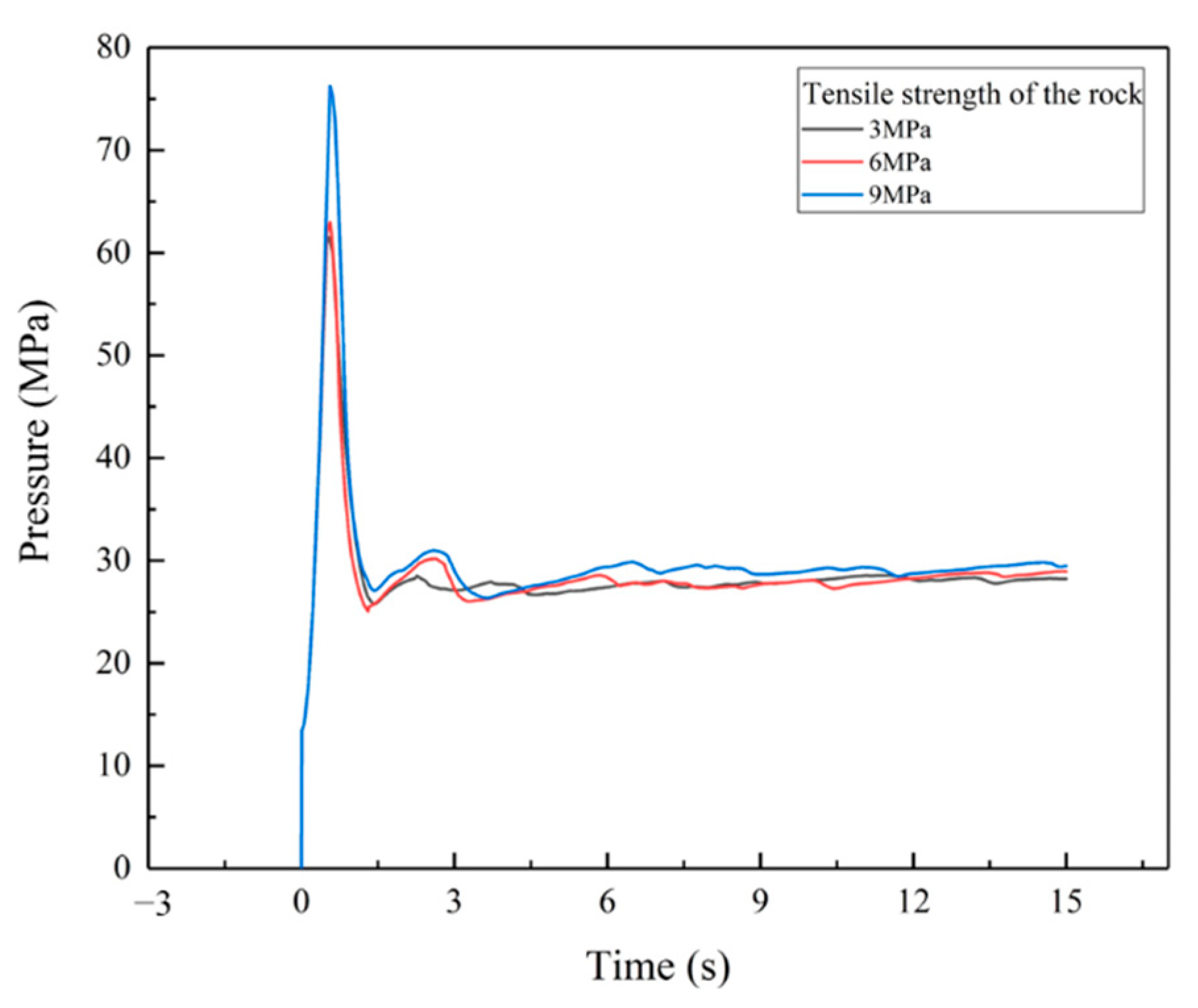
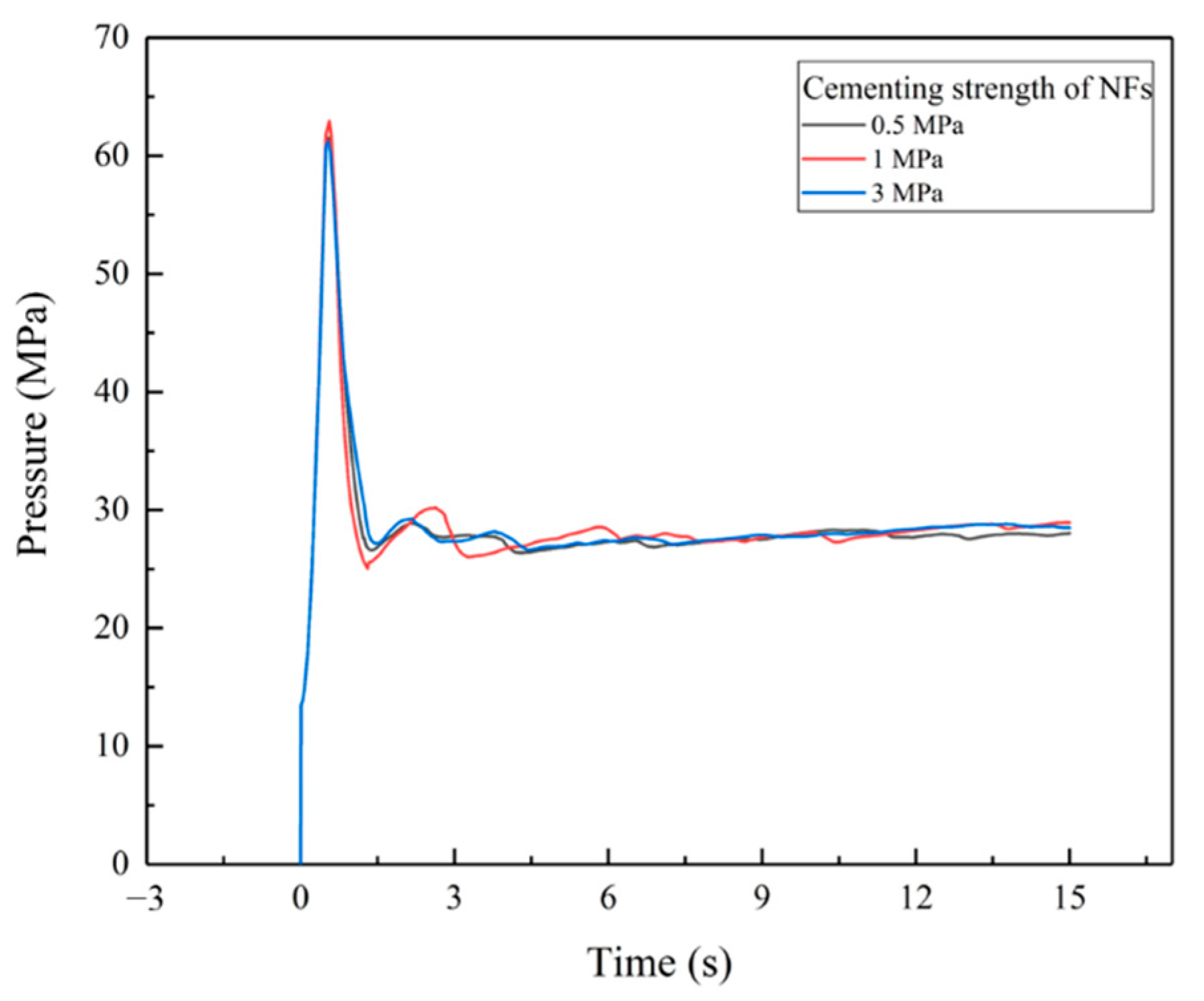
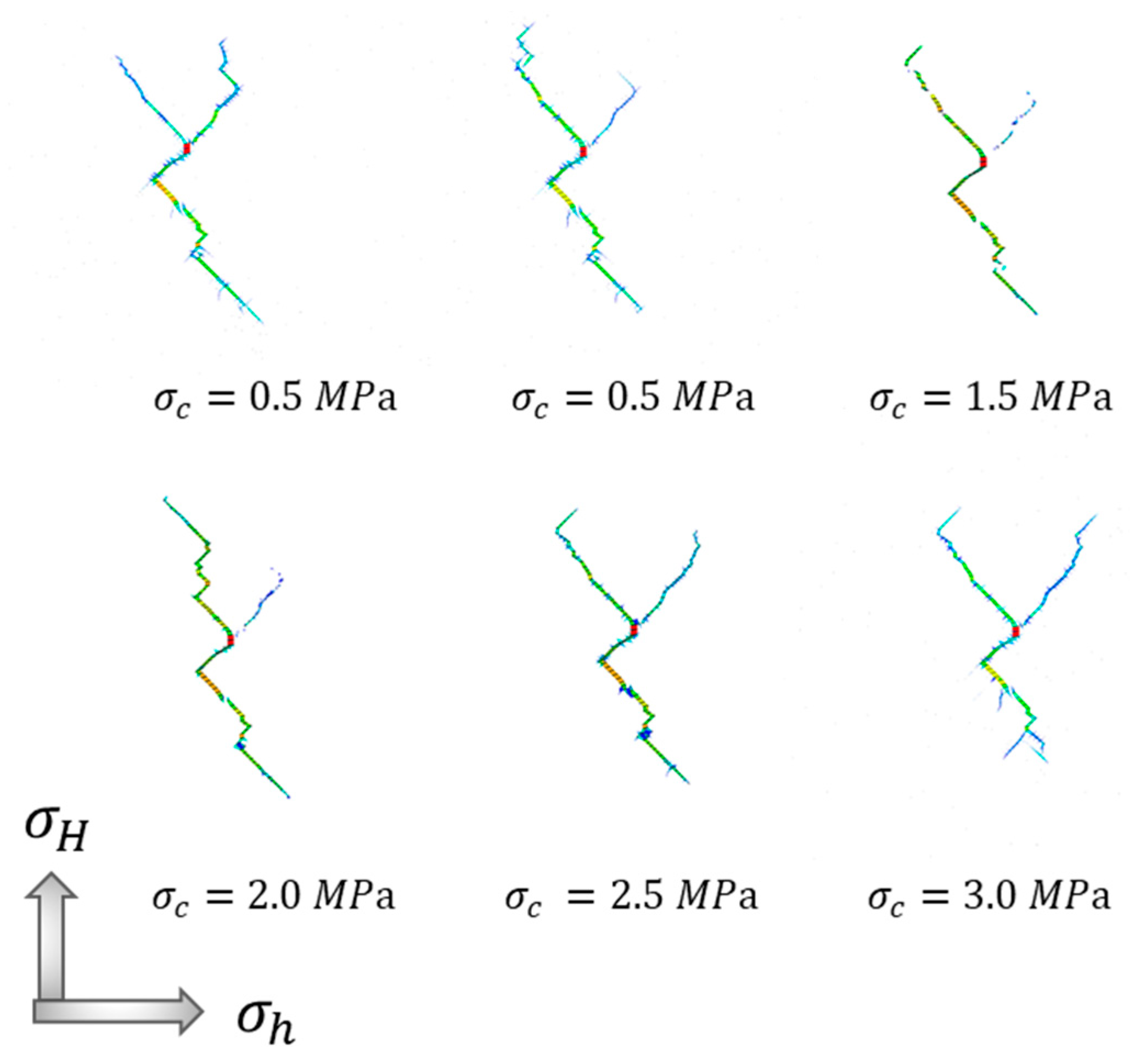
4.2. Tensile Strength of the Rock and Cementing Strength of Natural Fractures

The influence of the tensile strength of the rock σ t and the cementing strength natural fractures σ c on hydraulic fracture propagation were investigated. The in situ stress difference was kept at 5 MPa. In the cases of the sensitivity analysis of the rock tensile strength, σ t ranged from 3 MPa to 9 MPa, and σ c was 1 MPa. In the case of the sensitivity analysis of the cementing strength of the natural fractures, σ c was from 0.5 MPa to 3 MPam and σ t was 3 MPa. The simulation cases are listed in Table 2, and the results are represented in Figure 13, Figure 14, Figure 15 and Figure 16.
Figure 13 shows the extracted hydraulic fractures’ morphology under different rock tensile strengths. It indicates that the bifurcations and secondary fractures were diminished when the rock tensile strength was higher. To understand the propagation pattern of the hydraulic fractures, we analyzed the step-by-step fracture development when the rock tensile strength was 3 MPa, 6 MPa, and 9 MPa, as shown in Figure 14. When the tensile strength was 3 MPa, hydraulic fracturing produced a long left-sloping main fracture and a right-sloping secondary fracture. The secondary fracture propagated for a short distance and stopped. When the tensile strength of the rock was 6 MPa and 9 MPa, only the main fracture occurred, and the main fracture propagated in a zigzag fashion in the natural fracture network and rock matrix. The smaller the differences between the tensile strength of the rock and the natural fractures, the greater the possibility of hydraulic fracture propagated along the natural fractures. It can be seen from Figure 13 that when the tensile strength of rock was relatively small, the phenomenon of fracture bifurcation was more obvious, forming a secondary fracture and more bifurcations. This is because when the tensile strength of rock was higher, greater resistance was needed to overcome it to break up the rock, and fewer bifurcations occur, with a smaller fissured area.
The morphology of hydraulic fracturing fractures with different natural fracture mechanic properties is demonstrated in Figure 15. It can be seen from the figure that the hydraulic crack initiated from the perforation and formed a tri-wing fracture along the direction of the natural fracture. To understand the propagation pattern of the hydraulic fractures, we analyzed the step-by-step fracture development when the rock tensile strength was 0.5 MPa, 1.0 MPa, and 3.0 MPa, as shown in Figure 16. With the increase in the cementing strength of natural fractures, the length of the hydraulic crack on the lower side of perforation became shorter, and the number of bifurcated fractures turning to the rock matrix along the main fractures became larger.

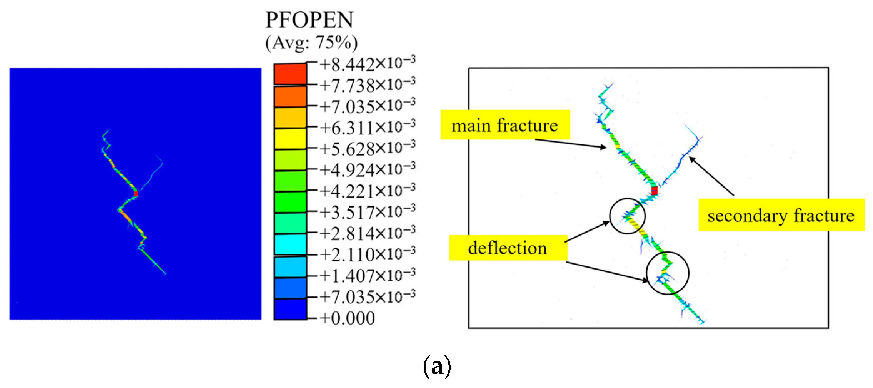
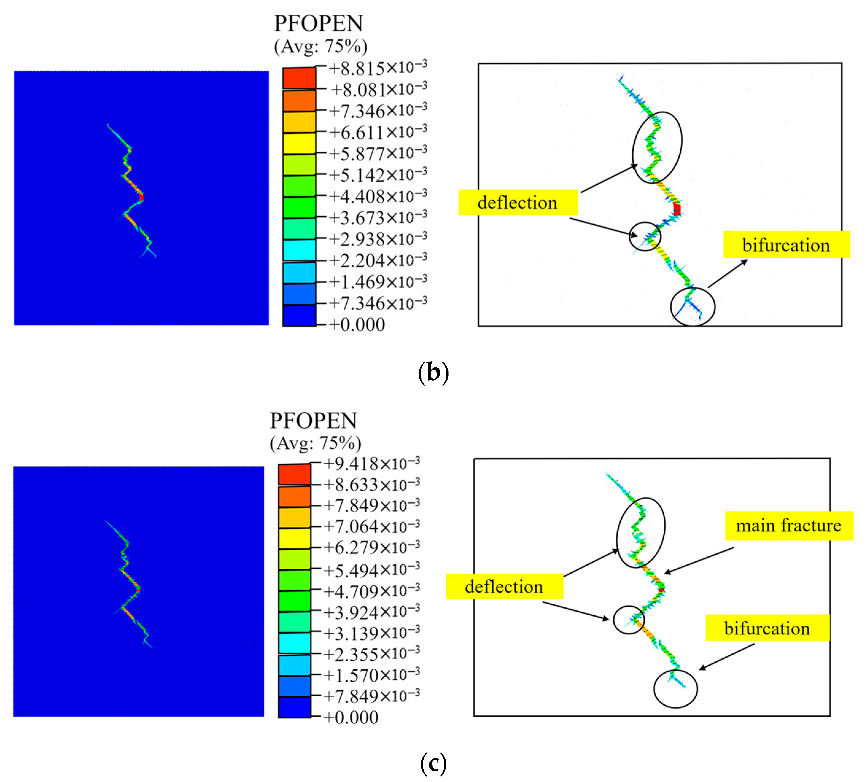
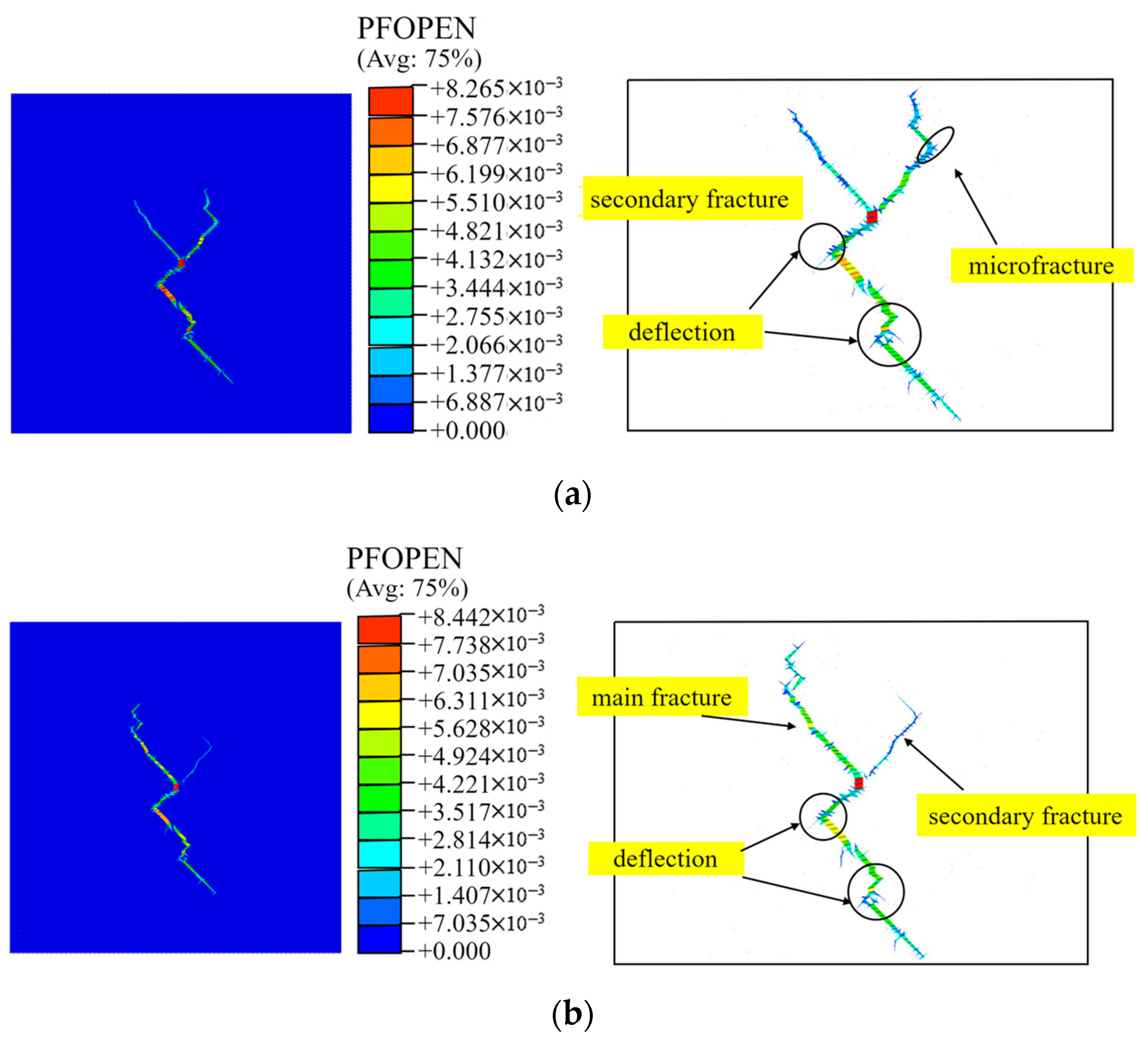
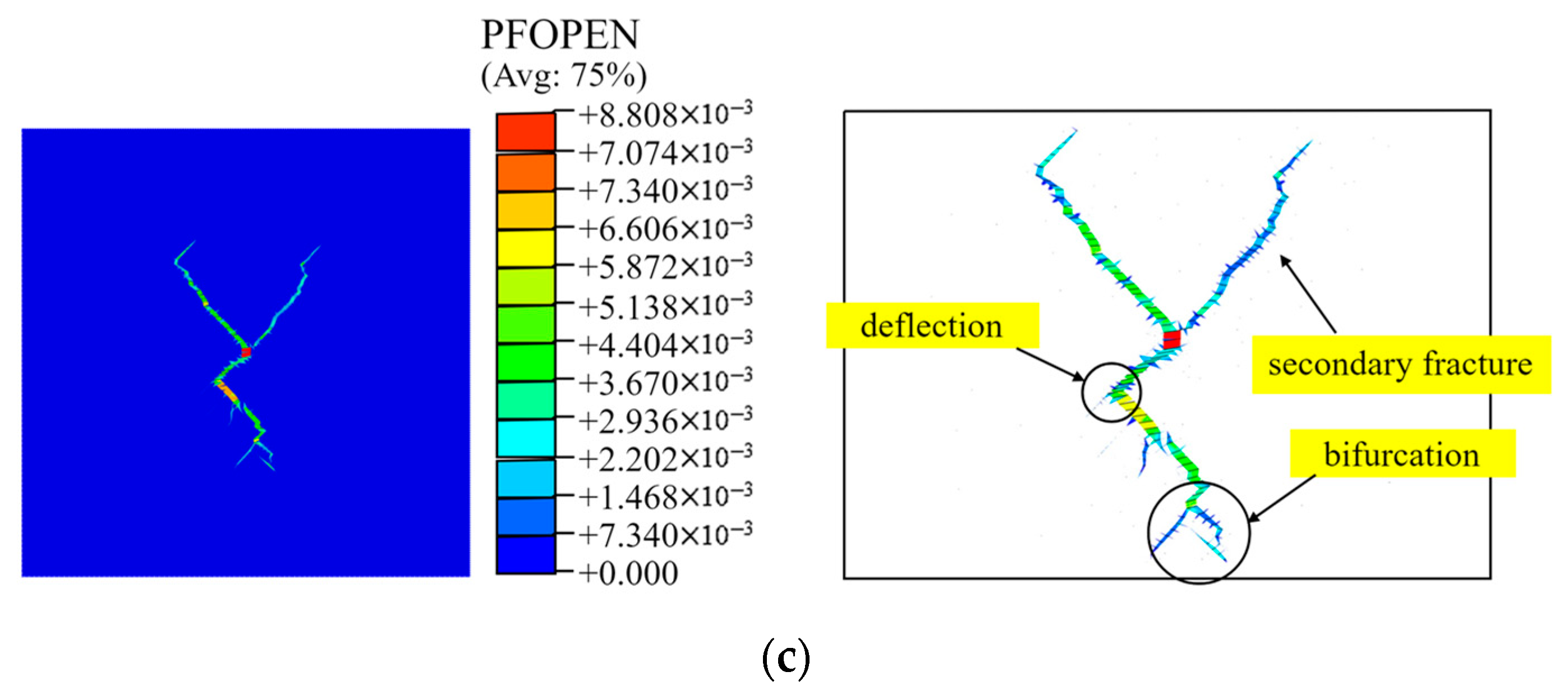
4.3. Complexity of Hydraulic Fracture Network

A complex fracture network is the key to obtaining considerable economic benefits. The formation of a complex network can enlarge the stimulated reservoir volume and cause the fluid in the matrix to permeate along the shortest distance, as well as reduce the driving pressure difference required for the oil and gas flow [50] Therefore, a quantitative assessment of the complexity of the fracture network is required. The total length of the main hydraulic fracture and the effective area of the fracture path in the model were extracted. Here, the effective area of the fracture path is defined as the total area of the closed area surrounded by the equivalent polyline of the hydraulic fracture, which can reflect the area influenced by different fracture shapes on a reservoir to a certain extent. In general, the effective area of reticulated fractures is larger than that of strip-type fractures, and the effective area of zigzag extended fractures is larger than that of unidirectional extended fractures.
The main fracture length and the effective area of a fracture path under different in situ stresses are summarized in Table 3 and Figure 17. With the increase in horizontal in situ stress difference, the length of the main fracture first increased and then declined. The maximum occurred when the horizontal in situ stress difference was 6 MPa, where the in situ stress ratio was 1.12, and the longest main fracture was 53.1 m. This indicates that an excessive horizontal in situ stress difference will lead to a single shape and direction of a hydraulic fracture, which is not conducive to the complexity of a fracture network. In general, the effective area of the fracture path decreased with the increase in the horizontal in situ stress difference. Its value was higher when the horizontal in situ stress difference was at a low level (0~2 MPa). This may be attributed to the secondary fracture with a large angle to the direction of the main fracture. The result shows that the key to increasing the complexity of the hydraulic fracture network is to form secondary fractures with a larger angle to the main fracture to enlarge the network morphology.
Figure 18 and Figure 19 show the length of the main fracture and maximum aperture under different tensile strengths of rock and cementing strengths of natural fractures, respectively. The fracture parameters are listed in Table 4. It can be seen that with the increase in rock tensile strength, the length of the main fracture decreased, in general. When the tensile strength of rock increased from 3 to 9 MPa, the length of the main fracture decreased from 40.4 to 35.1 m. This is because fracturing rock needs more energy when the tensile strength is higher, and it is difficult for a fracture to propagate in rock. Thus, excessive rock tensile strength is not conducive to stimulation treatments. It is better to select reservoirs with appropriate rock tensile strength for fracturing operations when conducting a fracturing feasibility study, for better economic benefits. In addition, it was found that the maximum aperture of the hydraulic fracture increased as the length of the crack decreased. This may because a longer length results in additional leak-off and reduces the fluid pressure in fractures [15], which makes the fracture more narrow.
Figure 19 shows the variation of the fracture length and maximum aperture of the hydraulic fracture under different cementing strengths of natural fractures. As shown in the figure, the length of the main fracture decreased with the increase in the cementing strength of natural fractures. When the cementing strength of natural fractures was 0.5 MPa, the length of the main fracture showed its maximum value and then decreased. Meanwhile, the maximum aperture of the hydraulic fracture increased as the cementing strength of the natural fractures increased. This is because the excessive cementing strength will make it difficult for hydraulic cracks to expand along natural fractures, which leads to the smaller length of the main fracture and more bifurcated fractures turning to rock matrix.

4.4. Bottom Hole Pressure

Bottom hole pressure is one of the most important indexes in oil and gas extraction. With the injection of fracturing fluid, the bottom hole pressure rises approximately linearly until it reaches the extreme point, which represents the breakdown pressure. A new fracture surface is formed after fracture initiation, and fracturing fluid fills the new fracture space, which results in a temporary decrease in bottom hole pressure. When the cohesive element at the fracture tip is completely damaged, the fracture propagates forward, and the pressure reaches a second peak. With the increase in fracture length, the fracturing fluid leak-off into the rock increases, and the pressure at the bottom of the well remains stable, finally. Bottom hole pressure curves under different in situ stress differences are shown in Figure 20. With the increase in in situ stress difference, the breakdown pressure decreased. Figure 21 and Figure 22 are bottom hole pressure curves under different rock tensile strengths and natural fracture cementing strengths, respectively. As can be seen from Figure 21, when the tensile strength of rock was 9 MPa, the initiation pressure was obviously higher than that of 6 MPa and 3 MPa. This is mainly because the greater the tensile strength of rock, the more energy is needed for fracturing the rock. As shown in Figure 22, the breakdown pressure did not change much when the cementing strength of natural cracks changed, because hydraulic fracture initiates in the rock and the breakdown pressure mainly depends on the mechanical parameters of reservoir.

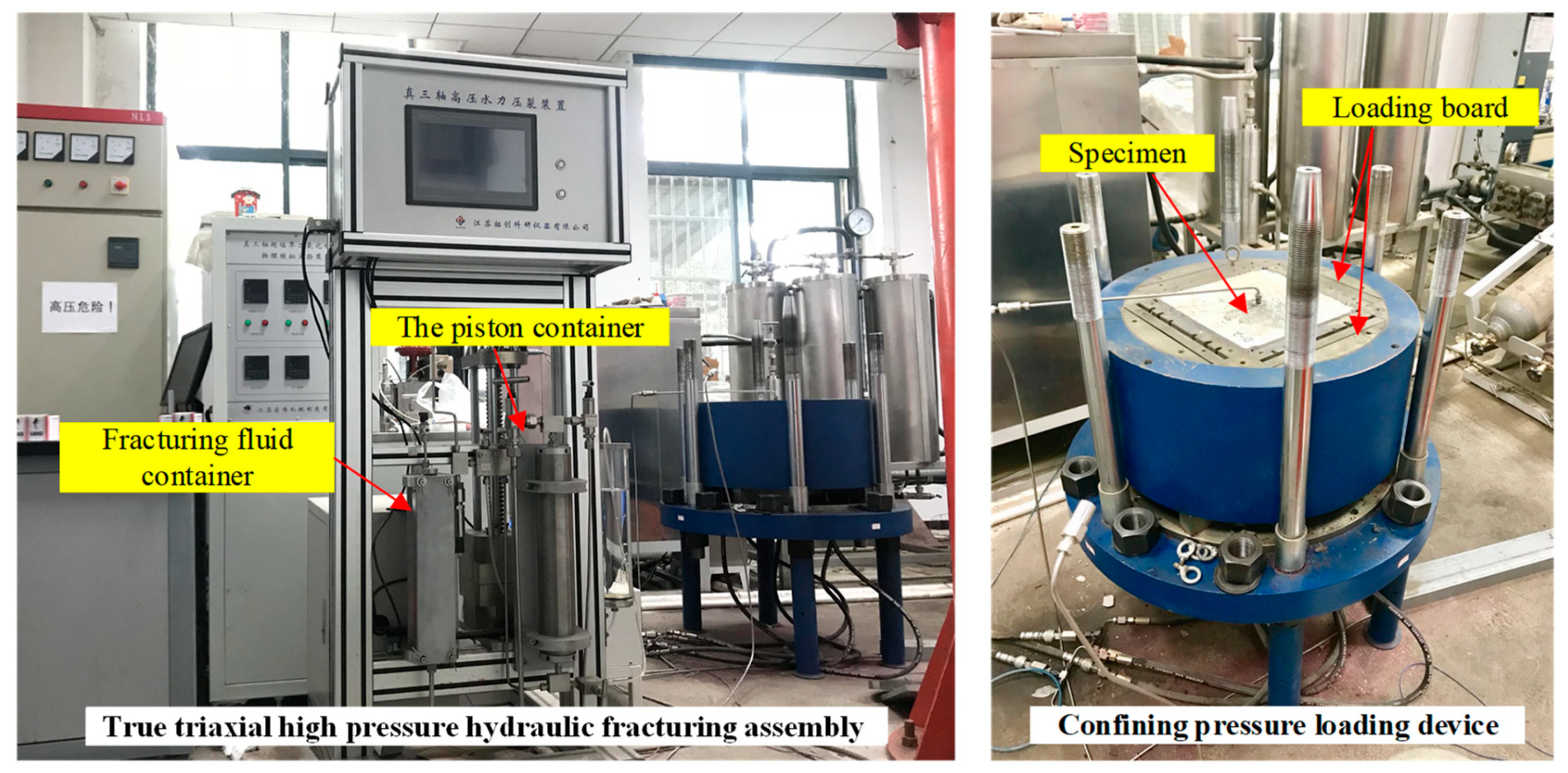
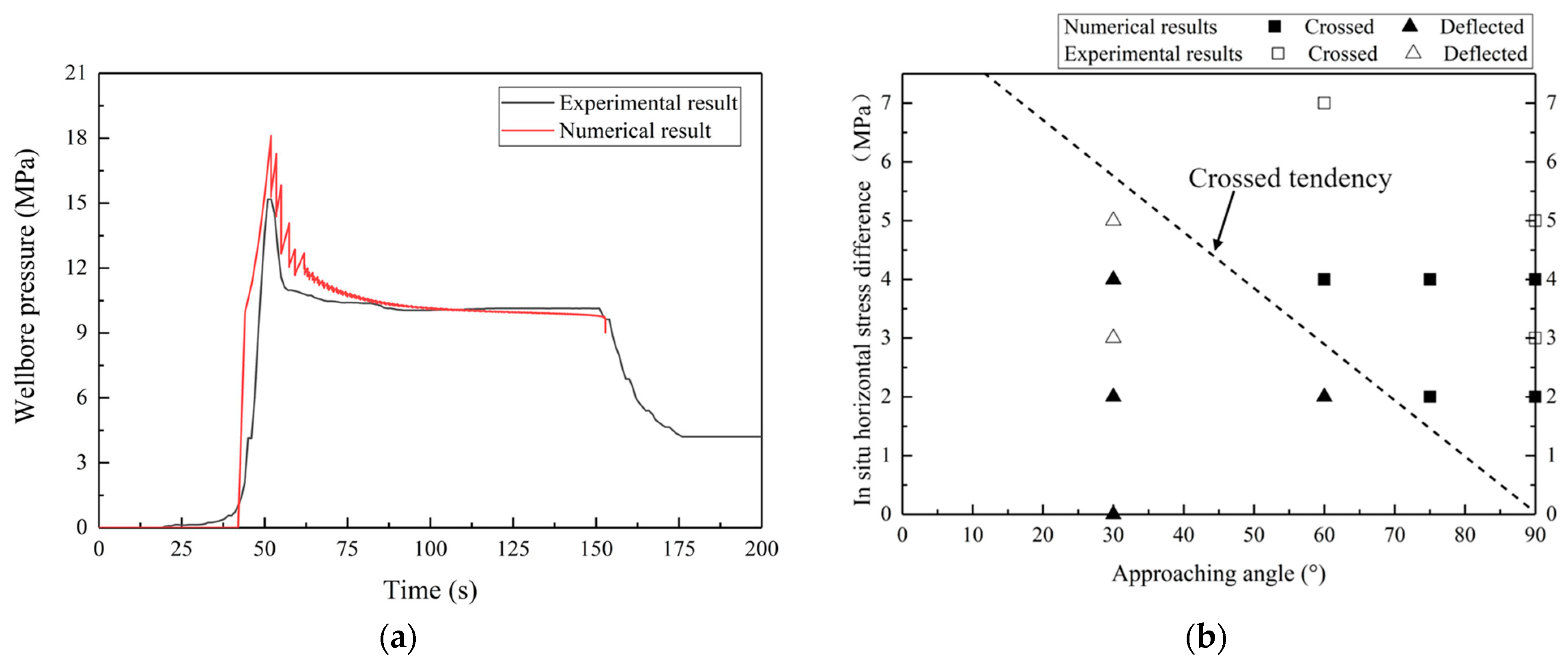
5. Verification Work

Some model validation work was conducted to verify the validation of simulating the hydraulic fracture interaction with natural fractures using the coupled pore fluid diffusion and stress analysis along with global cohesive element.
Firstly, we compared the simulation results with a triaxial hydraulic fracturing experiment in the laboratory. A true triaxial fracturing system was used to perform hydraulic fracturing on synthetic rock specimens that had been strictly prepared and cured (Figure 23). The cubic model block with a side length of 300 mm was located in a confining pressure loading device, which was used to simulate the field stress conditions. Three independent double cylinder hydraulic pump sets provided dynamic confining pressure loading. The test parameters referred to the field test parameters and were calculated by similarity criteria. The vertical, maximum, and minimum horizontal principal stresses were 9.8 MPa, 10.5 MPa and 8.6 MPa, respectively. The hydraulic fluid injection pressure was controlled by the hydraulic pump of the hydraulic fracturing assembly. The injection rate was 1 mL/s. As a control group, a fluid–solid coupled model was established with the same parameters used in the experiment, and the simulation result was compared with the experimental result. The results showed that the bottom hole pressure curve obtained by the numerical simulation was highly consistent with the bottom hole pressure curve in the experiment, shown in Figure 24a. The breakdown pressure and steady pressure obtained from the simulation were 17.38 MPa and 9.92 MPa relatively, which were very close to the experimental results of 15.18 MPa and 10.08 MPa. It proved that simulating the hydraulic fracturing using coupled pore fluid diffusion and stress analysis is credible.
Another model was used to verify the accuracy of the interaction between hydraulic fractures and natural fractures. Different scenarios might occur in the interaction of a hydraulic fracture and a pre-existing natural fracture in naturally fractured shale reservoirs [23,51,52]. The hydraulic fracture may deflect into the natural fracture under the influence of the pre-existing fracture, or it may cross directly without being impacted by the natural fracture. The numerical model was built to simulate the intersection behavior of a hydraulic fracture and a single pre-existing natural fracture. A cohesive pore pressure element was inserted into the model to serve as the natural fracture, and coupled pore fluid diffusion and stress analysis were used to simulate the solid–fluid problem. By changing the in situ horizontal stress difference and the approximation angle, different propagation behaviors of hydraulic fractures were obtained. The numerical results and the experimental results are shown in Figure 24b. Square data denote that the hydraulic fracture crossed the natural fracture, while triangle data denote that the hydraulic fracture was captured and deflected to the direction of the natural fracture. At a small approaching angle, the experimental results and the simulation results showed that hydraulic fractures were deflected. When the approaching angle was 60°, the numerical results showed that the hydraulic fracture deflected under 2 MPa in situ stress difference and crossed under 4 MPa in situ stress difference. At higher approaching angles, the numerical results agreed with the experimental results that the hydraulic fractures crossed the natural fracture. In general, the simulation cases were consistent with the experimental cases in the literature [53]. This shows that it is effective to simulate fracture intersection behavior by using cohesive element combined with coupled pore fluid diffusion and stress analysis.

6. Summary and Conclusions

In this paper, a global cohesive model was established to simulate the natural fracture network in a reservoir. The propagation patterns of a hydraulic fracture in a natural fracture network were investigated. The propagation, bifurcation, and intersection of a hydraulic fracture under different in situ horizontal stress differences, the tensile strengths of rock, and cementing strengths of natural fractures were studied. The fracture parameters such as length and maximum aperture and the effective area of the fracture path were quantitatively evaluated. The results can be briefly concluded as follows:
(1)
The global cohesive model can achieve non-prefabricated propagation of hydraulic fractures in a natural fracture network. This contributes a fracture simulation close to that in a real situation and benefits the understanding of the role that natural fractures play in induced-fracture propagation.
(2)
Step-by-step propagation patterns of hydraulic fractures showed that the hydraulic fracture tips were attracted by local natural fractures under low in situ stress difference. This led to bifurcations and secondary fractures at the intersection of fractures and, thus, contributed to the complexity of the induced fracture network. The influence of natural fractures on the overall trend of fracture propagation was limited when the in situ stress difference increased.
(3)
An effective area that indicated the influenced area of induced fractures was defined. It was higher when the horizontal in situ stress difference was at a low level, due to the formation of secondary fractures. When the in situ stress ratio was 1.12, the length of the main hydraulic fracture reached its maximum.
(4)
The mechanical properties of rock and natural fractures have impacts on the propagation of induced fractures. With the increase in the tensile strength of rock and the cementing strength of natural fractures, the induced fracture became less complicated due to the high cracking energy, and the length of the main fracture decreased. In addition, the higher tensile strength of rock increased the initiation pressure of the induced fracture, while the cementing strength of the natural fractures showed no impact on it.
The results of the study can be utilized to explain various hydraulic fracturing behaviors in reservoirs that developed with rich natural fractures. It allows for the prediction of induced fracture propagations as well as the connection with natural fractures. The method can be utilized for related fracturing design, in general. In the future, the anisotropy of rock and the temperature stress field should be considered in study to obtain results that fit real situations.

Author Contributions

Conceptualization, Y.L.; methodology, Y.H.; simulation, Y.L.; validation, Y.L.; writing—original draft preparation, Y.L.; writing—review and editing, Y.K. All authors have read and agreed to the published version of the manuscript.

Funding

This work is supported by the National Natural Science Foundation of China (No. 52174004), the National Key Research and Development, Program of China (No. 2018YFC0808401), and the Fundamental Research Funds for the Central Universities (2042022kf1025).

Institutional Review Board Statement

Not applicable.

Informed Consent Statement

Not applicable.

Data Availability Statement

Not applicable.

Conflicts of Interest

The authors declare no conflict of interest. The funders had no role in the design of the study; in the collection, analyses, or interpretation of data; in the writing of the manuscript, or in the decision to publish the results.

References

  1. Cheng, W.; Jin, Y.; Chen, M. Experimental study of step-displacement hydraulic fracturing on naturally fractured shale outcrops. J. Geophys. Eng. 2015, 12, 714–723. [Google Scholar] [CrossRef]
  2. Bunger, A.P.; Zhang, X.; Jeffrey, R.G. Parameters affecting the interaction among closely spaced hydraulic fractures. Spe J. 2012, 17, 292–306. [Google Scholar] [CrossRef]
  3. Gale, J.F.W.; Laubach, S.E.; Olson, J.E.; Eichhubl, P.; Fall, A. Natural fractures in shale: A review and new observationsNatural Fractures in Shale: A Review and New Observations. Am. Assoc. Pet. Geol. Bull. 2014, 98, 2165–2216. [Google Scholar]
  4. Mayerhofer, M.J.; Lolon, E.; Warpinski, N.R.; Cipolla, C.L.; Walser, D.W.; Rightmire, C.M. What is stimulated rock volume. In Proceedings of the SPE Asia Pacific Unconventional Resources Conference and Exhibition, Brisbane, Qld, Australia, 18–20 October 2010. [Google Scholar]
  5. Keshavarzi, R.; Mohammadi, S.; Bayesteh, H. Hydraulic fracture propagation in unconventional reservoirs: The role of natural fractures. In Proceedings of the 46th US Rock Mechanics/Geomechanics Symposium, Chicago, IL, USA, 24–27 June 2012. [Google Scholar]
  6. Rutledge, J.T.; Phillips, W.S.; Mayerhofer, M.J. Faulting induced by forced fluid injection and fluid flow forced by faulting: An interpretation of hydraulic-fracture microseismicity, Carthage Cotton Valley gas field, Texas. Bull. Seismol. Soc. Am. 2004, 94, 1817–1830. [Google Scholar] [CrossRef]
  7. Wasantha, P.L.P.; Konietzky, H.; Weber, F. Geometric nature of hydraulic fracture propagation in naturally-fractured reservoirs. Comput. Geotech. 2017, 83, 209–220. [Google Scholar] [CrossRef]
  8. Fatahi, H.; Hossain, M.M.; Sarmadivaleh, M. Numerical and experimental investigation of the interaction of natural and propagated hydraulic fracture. J. Nat. Gas Sci. Eng. 2017, 37, 409–424. [Google Scholar] [CrossRef] [Green Version]
  9. Dahi Taleghani, A.; Gonzalez, M.; Shojaei, A. Overview of numerical models for interactions between hydraulic fractures and natural fractures: Challenges and limitations. Comput. Geotech. 2016, 71, 361–368. [Google Scholar] [CrossRef]
  10. Maxwell, S.C.; Urbancic, T.I.; Steinsberger, N.; Zinno, R. Microseismic imaging of hydraulic fracture complexity in the Barnett shale. In Proceedings of the SPE Annual Technical Conference and Exhibition, San Antonio, TX, USA, 29 September 2002. [Google Scholar]
  11. Renshaw, C.E.; Pollard, D.D. An experimentally verified criterion for propagation across unbounded frictional interfaces in brittle, linear elastic materials. In International Journal of Rock Mechanics and Mining Sciences & Geomechanics Abstracts; Pergamon: Oxford, UK, 1995; Volume 32, pp. 237–249. [Google Scholar]
  12. Gu, H.; Weng, X.; Lund, J.; Mack, M.; Ganguly, U.; Suarez-Rivera, R. Hydraulic fracture crossing natural fracture at nonorthogonal angles: A criterion and its validation. SPE Prod. Oper. 2012, 27, 20–26. [Google Scholar] [CrossRef]
  13. Bahorich, B.; Olson, J.E.; Holder, J. Examining the effect of cemented natural fractures on hydraulic fracture propagation in hydrostone block experiments. In Proceedings of the SPE Annual Technical Conference and Exhibition, San Antonio, TX, USA, 8–10 October 2012. [Google Scholar]
  14. Soliman, M.Y.; Daal, J.; East, L. Fracturing unconventional formations to enhance productivity. J. Nat. Gas Sci. Eng. 2012, 8, 52–67. [Google Scholar] [CrossRef]
  15. Warpinski, N.R.; Teufel, L.W. Influence of geologic discontinuities on hydraulic fracture propagation. J. Pet. Technol. 1987, 39, 209–220. [Google Scholar] [CrossRef]
  16. Olson, J.E.; Dahi-Taleghani, A. Modeling simultaneous growth of multiple hydraulic fractures and their interaction with natural fractures. In Proceedings of the SPE Hydraulic Fracturing Technology Conference, The Woodlands, TX, USA, 19 January 2009. [Google Scholar] [CrossRef]
  17. McClure, M.W. Modeling and Characterization of Hydraulic Stimulation and Induced Seismicity in Geothermal and Shale Gas Reservoirs; Stanford University: Stanford, CA, USA, 2012. [Google Scholar]
  18. Xu, G.; Wong, S.-W. Interaction of multiple non-planar hydraulic fractures in horizontal wells. In Proceedings of the IPTC 2013: International Petroleum Technology Conference, Beijing, China, 26–28 March 2013; p. cp-350-00461. [Google Scholar]
  19. Castonguay, S.T.; Mear, M.E.; Dean, R.H.; Schmidt, J.H. Predictions of the growth of multiple interacting hydraulic fractures in three dimensions. In Proceedings of the SPE Annual Technical Conference and Exhibition, New Orleans, LA, USA, 30 September 2013. [Google Scholar]
  20. Hossain, M.M.; Rahman, M.K. Numerical simulation of complex fracture growth during tight reservoir stimulation by hydraulic fracturing. J. Pet. Sci. Eng. 2008, 60, 86–104. [Google Scholar] [CrossRef]
  21. Chen, Z. Finite element modelling of viscosity-dominated hydraulic fractures. J. Pet. Sci. Eng. 2012, 88, 136–144. [Google Scholar] [CrossRef]
  22. Shin, D.H.; Sharma, M.M. Factors controlling the simultaneous propagation of multiple competing fractures in a horizontal well. In Proceedings of the SPE Hydraulic Fracturing Technology Conference, The Woodlands, TX, USA, 4–6 February 2014. [Google Scholar]
  23. Taleghani, A.D.; Olson, J.E. How natural fractures could affect hydraulic-fracture geometry. SPE J. 2014, 19, 161–171. [Google Scholar] [CrossRef]
  24. Weber, N.; Siebert, P.; Willbrand, K.W.; Feinendegen, M.; Clauser, C.; Fries, T.-P. The XFEM with an explicit-implicit crack description for hydraulic fracture problems. In Proceedings of the ISRM International Conference for Effective and Sustainable Hydraulic Fracturing, Brisbane, Australia, 20 May 2013. [Google Scholar]
  25. Nagel, N.B.; Sanchez-Nagel, M.; Lee, B. Gas shale hydraulic fracturing: A numerical evaluation of the effect of geomechanical parameters. In Proceedings of the SPE Hydraulic Fracturing Technology Conference, The Woodlands, TX, USA, 6–8 February 2012. [Google Scholar]
  26. Savitski, A.A.; Lin, M.; Riahi, A.; Damjanac, B.; Nagel, N.B. Explicit modeling of hydraulic fracture propagation in fractured shales. In Proceedings of the IPTC 2013: International Petroleum Technology Conference, Beijing, China, 26–28 March 2013; p. cp-350-00477. [Google Scholar]
  27. Hyman, J.D.; Karra, S.; Makedonska, N.; Gable, C.W.; Painter, S.L.; Viswanathan, H.S. dfnWorks: A discrete fracture network framework for modeling subsurface flow and transport. Comput. Geosci. 2015, 84, 10–19. [Google Scholar] [CrossRef] [Green Version]
  28. Riahi, A.; Damjanac, B. Numerical study of interaction between hydraulic fracture and discrete fracture network. In Proceedings of the ISRM International Conference for Effective and Sustainable Hydraulic Fracturing, Brisbane, Australia, 20 May 2013. [Google Scholar]
  29. Damjanac, B.; Cundall, P. Application of distinct element methods to simulation of hydraulic fracturing in naturally fractured reservoirs. Comput. Geotech. 2016, 71, 283–294. [Google Scholar] [CrossRef]
  30. Haddad, M.; Sepehrnoori, K. Simulation of hydraulic fracturing in quasi-brittle shale formations using characterized cohesive layer: Stimulation controlling factors. J. Unconv. Oil Gas Resour. 2015, 9, 65–83. [Google Scholar] [CrossRef]
  31. Pouya, A.; Yazdi, P.B. A damage-plasticity model for cohesive fractures. Int. J. Rock Mech. Min. Sci. 2015, 73, 194–202. [Google Scholar] [CrossRef]
  32. Guo, J.; Zhao, X.; Zhu, H.; Zhang, X.; Pan, R. Numerical simulation of interaction of hydraulic fracture and natural fracture based on the cohesive zone finite element method. J. Nat. Gas Sci. Eng. 2015, 25, 180–188. [Google Scholar] [CrossRef]
  33. Gonzalez, M.; Dahi Taleghani, A.; Olson, J.E. A cohesive model for modeling hydraulic fractures in naturally fractured formations. In Proceedings of the SPE Hydraulic Fracturing Technology Conference, The Woodlands, TX, USA, 3–5 February 2015; pp. 858–873. [Google Scholar] [CrossRef]
  34. Chen, Z.; Bunger, A.P.; Zhang, X.; Jeffrey, R.G. Cohesive zone finite element-based modeling of hydraulic fractures. Acta Mech. Solida Sin. 2009, 22, 443–452. [Google Scholar] [CrossRef]
  35. Sarris, E.; Papanastasiou, P. Modeling of hydraulic fracturing in a poroelastic cohesive formation. Int. J. Geomech. 2012, 12, 160–167. [Google Scholar] [CrossRef]
  36. Elices, M.; Guinea, G.V.; Gomez, J.; Planas, J. The cohesive zone model: Advantages, limitations and challenges. Eng. Fract. Mech. 2002, 69, 137–163. [Google Scholar] [CrossRef]
  37. Terzaghi, K.; Peck, R.B.; Mesri, G. Soil Mechanics in Engineering Practice; John Wiley & Sons: New York, NY, USA, 1996. [Google Scholar]
  38. Tariq, S.M. Evaluation of flow characteristics of perforations including nonlinear effects with the finite-element method. SPE Prod. Eng. 1987, 2, 104–112. [Google Scholar] [CrossRef]
  39. Erdogan, F.; Sih, G.C. On the crack extension in plates under plane loading and transverse shear. J. Basic Eng. 1963, 85, 519–525. [Google Scholar] [CrossRef]
  40. Maiti, S.K.; Smith, R.A. Comparison of the criteria for mixed mode brittle fracture based on the preinstability stress-strain field Part I: Slit and elliptical cracks under uniaxial tensile loading. Int. J. Fract. 1983, 23, 281–295. [Google Scholar] [CrossRef]
  41. Hussain, M.A.; Pu, L.; Underwood, J. Strain Energy Release Rate for a crack under combined mode I and mode II. In Proceedings of the 1973 National Symposium on Fracture Mechanics, University of Maryland, College Park, Maryland, 27–29 August 1973; Volume 559, p. 2. [Google Scholar]
  42. Sih, G.C. Some basic problems in fracture mechanics and new concepts. Eng. Fract. Mech. 1973, 5, 365–377. [Google Scholar] [CrossRef]
  43. Sidoroff, F. Description of anisotropic damage application to elasticity. In Physical Non-Linearities in Structural Analysis; Springer: Heidelberg, Germany, 1981; pp. 237–244. [Google Scholar]
  44. Gurson, A.L. Continuum theory of ductile rupture by void nucleation and growth: Part I—Yield criteria and flow rules for porous ductile media. J. Eng. Mater. Technol. 1977, 99, 2–15. [Google Scholar] [CrossRef]
  45. Zhaoxia, L.; Liguang, X. Finite element analysis of local damage and post-failure behavior for strain-softening solid. Int. J. Fract. 1996, 80, 85–95. [Google Scholar] [CrossRef]
  46. Camanho, P.P.; Dávila, C.G. Mixed-Mode Decohesion Finite Elements for the Simulation of Delamination in Composite Materials; National Aeronautics and Space Administration (NASA): Washington, DC, USA, 2002. [Google Scholar]
  47. Carpinteri, A. Nonlinear Crack Models for Nonmetallic Materials; Springer Science & Business Media: New York, NY, USA, 2012; Volume 71. [Google Scholar]
  48. Cornec, A.; Scheider, I.; Schwalbe, K.-H. On the practical application of the cohesive model. Eng. Fract. Mech. 2003, 70, 1963–1987. [Google Scholar] [CrossRef]
  49. Wang, Z.; Sun, J. Exploitation Practice and Cognition of Pilot Well Group in Fuling Shale Gas Field; China Petrochemical Press: Beijing, China, 2014. [Google Scholar]
  50. Maxwell, S.C.; Waltman, C.; Warpinski, N.R.; Mayerhofer, M.J.; Boroumand, N. Imaging seismic deformation induced by hydraulic fracture complexity. SPE Reserv. Eval. Eng. 2009, 12, 48–52. [Google Scholar] [CrossRef] [Green Version]
  51. Fu, W.; Ames, B.C.; Bunger, A.P.; Savitski, A.A. An experimental study on interaction between hydraulic fractures and partially-cemented natural fractures. In Proceedings of the 49th US Rock Mechanics/Geomechanics Symposium, San Francisco, CA, USA, 29 June–1 July 2015. [Google Scholar]
  52. Jeffrey, R.G.; Zhang, X.; Thiercelin, M.J. Hydraulic fracture offsetting in naturally fractures reservoirs: Quantifying a long-recognized process. In Proceedings of the SPE Hydraulic Fracturing Technology Conference, The Woodlands, TX, USA, 19 January 2009. [Google Scholar]
  53. Zhou, J.; Chen, M.; Jin, Y.; Zhang, G. Analysis of fracture propagation behavior and fracture geometry using a tri-axial fracturing system in naturally fractured reservoirs. Int. J. Rock Mech. Min. Sci. 2008, 45, 1143–1152. [Google Scholar] [CrossRef]
Figure 1. Schematic of the intersection between a hydraulic fracture and a natural fracture using pore pressure cohesive elements. Inspired by [32].
Applsci 12 04738 g001
Figure 2. Cohesive traction–separation law with linear damage evolution.
Applsci 12 04738 g002
Figure 3. (a). Schematic of two-dimensional pore pressure cohesive element. (b) Fluid flow in cohesive element. The pore pressure cohesive element can simulate a tangential flow and leak-off from fracture to rock matrix.
Applsci 12 04738 g003
Figure 4. Schematic of arrangement of cohesive elements at the intersection of a hydrofracture with a fixed propagation direction and a pre-existing natural fracture.
Applsci 12 04738 g004
Figure 5. Schematic of element nodes at the intersection.
Applsci 12 04738 g005
Figure 6. Schematic representation of discontinuous natural fractures network model.
Applsci 12 04738 g006
Figure 7. Schematic diagram of the natural fractures network model established using global cohesive elements. (a) Mesh generation of the natural fractures network model. (b) The mesh is locally enlarged to show the location of the natural fracture more clearly. (c) Mesh before embedding cohesive element. (d) Mesh after global embedding cohesive elements.
Applsci 12 04738 g007
Figure 8. The extracted morphology of hydraulic fractures under different in situ stress differences.
Applsci 12 04738 g008
Figure 9. The in situ stress difference at 0 MPa. (a) Schematic diagram of the fracture morphology. (b) The propagation process of the hydrofractures in a natural fracture network.
Applsci 12 04738 g009
Figure 10. The in situ stress difference at 5 MPa. (a) Schematic diagram of the fracture morphology. (b) The propagation process of the hydrofractures in a natural fracture network.
Applsci 12 04738 g010
Figure 11. The in situ stress difference at 10 MPa. (a) Schematic diagram of the fracture morphology. (b) The propagation process of the hydrofractures in a natural fracture network.
Applsci 12 04738 g011aApplsci 12 04738 g011b
Figure 12. The in situ stress difference at 15 MPa. (a) Schematic diagram of the fracture morphology. (b) The propagation process of the hydrofractures in a natural fracture network.
Applsci 12 04738 g012
Figure 13. The extracted morphology of hydraulic fractures under different rock tensile strengths.
Applsci 12 04738 g013
Figure 14. Schematic diagram of fracture morphology in different tensile strength of rock. (a) 3 MPa. (b) 6 MPa. (c) 9 MPa.
Applsci 12 04738 g014aApplsci 12 04738 g014b
Figure 15. The extracted morphology of hydraulic fractures under different cementing strengths of natural fractures.
Applsci 12 04738 g015
Figure 16. Schematic diagram of fracture morphology in different interface cementing strengths of natural fractures. (a) 0.5 MPa. (b) 1 MPa. (c) 3 MPa.
Applsci 12 04738 g016aApplsci 12 04738 g016b
Figure 17. Fracture length under different in situ horizontal stresses.
Applsci 12 04738 g017
Figure 18. Fracture length under different tensile strengths of rock.
Applsci 12 04738 g018
Figure 19. Fracture length under different cementing strengths of a natural fracture.
Applsci 12 04738 g019
Figure 20. The bottom hole pressure under different in situ horizontal stresses.
Applsci 12 04738 g020
Figure 21. The bottom hole pressure under different tensile strengths of rock.
Applsci 12 04738 g021
Figure 22. The bottom hole pressure under different cementing strengths of natural fractures.
Applsci 12 04738 g022
Figure 23. Schematic of the triaxial hydraulic fracturing test system used in the experiment.
Applsci 12 04738 g023
Figure 24. (a) Result comparison between the numerical simulation and the physical experiment. (b) Result comparison between the numerical simulation and the simulation in the reference.
Applsci 12 04738 g024
Table 1. Relevant parameters for the model.
ParameterValueParameterValue
Young’s modulus30.2 GPaInitial pore pressure36.5 MPa
Poisson’s ratio0.2Porosity0.1
Tensile strength of the rock3/6/9 MPaPermeability coefficient2.23 × 10−7 m/s
Cementing strength of the NFs 10.5/1/3 MPaLeak-off coefficient1 × 10−13 m/(Pa·s)
Minimum in situ horizontal stress50 MPaInjection rate0.01 m3/s
Maximum in situ horizontal stress65 MPaFluid viscosity0.001 Pa·s
1 NFs means natural fractures.
Table 2. Simulation cases.
Case
Tensile strength of the rock σ t = 3, 4, 5, 6, 7, 8, 9 MPa
Cementing strength of NFs 1 (MPa) σ c = 0.5, 1, 1.5, 2.0, 2.5, 3.0 MPa
σ H σ h 5 MPa
1 NFs denotes natural fractures.
Table 3. Fracture parameters under different horizontal stresses.
σ H σ h ( MPa ) σ H / σ h Length of Main Fractures (m)Effective Area of Fracture Path (m2)
01.037.3123.7
11.0243.1126.4
21.0440.5122.3
31.0645.492.6
41.0847.686.7
51.1048.762.4
61.1253.190.3
71.1448.447.2
81.1642.526.1
91.1844.137.4
101.2041.923.9
111.2239.624.1
121.2440.233.5
131.2641.234.1
141.2843.145.2
151.3040.337.5
Table 4. Fracture parameters under different tensile strengths of rock and cementing strengths of natural fractures.
σ t ( MPa ) σ c   ( M P a ) Length of Main Fractures (m)Maximum Aperture (10−3 m)
31.040.48.442
41.038.68.601
51.037.98.900
61.037.78.815
71.035.58.896
81.036.29.242
91.035.19.418
30.541.18.265
31.539.68.532
32.039.18.682
32.537.38.735
33.035.58.808
Publisher’s Note: MDPI stays neutral with regard to jurisdictional claims in published maps and institutional affiliations.

