An Effective Beam Width Model of Slab in Thick Wall-Thick Slab Joints Subjected to Lateral Forces

Featured Application

This proposed effective beam width model was developed for predicting the initial stiffness of the wall-slab joints for providing a simplified way to determine whether a wall-slab joint satisfied the seismic stiffness requirements.

Abstract

Thick wall-thick slab structures are a newly-developed type of structural system comprising solely of structural floor slabs and shear walls, the former of which is thicker than that of slabs used in typical reinforced concrete frame structures. This study looks to develop a method to predict the initial stiffness of thick wall-thick slab joints under lateral loading by adopting the effective beam width method (EBWM). The height and length of the bearing wall, and the span length of the slab on effective beam width have been considered. Moreover, a correction coefficient that estimates the lateral force applied on the wall top, which is another crucial parameter for predicting the effective beam width and considered as the condition providing initial stiffness, is suggested based on experimental data from the literature. Additionally, by comparing values of the effective beam width obtained from the proposed model with those calculated using equations employed by the current code according to three wall-slab joint specimens, it has been demonstrated the usefulness and accuracy of the proposed method, which works better than the current code method for the wall-slab joints in TWTS cases.

1. Introduction

In Japan, conventional reinforced concrete wall (WRC) structures, such as described in Inoue and Teshigawara ‘s work [1] and as shown in Figure 1, are composed of bearing walls, floor slabs, and protruding beams connected to the walls (called “wall beam” in the following contents). This type of structural system was invented in Japan after World War II as a result of the Japanese Government needing to provide a large number of residential buildings with good structural performance and a comfortable living environment [2,3]. This type of system had many benefits such as ease of mass production, good fire resistance, and high seismic resistance, resulting in the WRC structural system still being commonly used in current practice [1,3]. In particular, the high seismic performance is one of the most important features given that Japan is located in one of the most active seismic zones globally. In several major seismic events since the widespread adoption of WRC buildings, such as the Tohoku earthquake in 2011 and Kumamoto earthquake in 2016, it was observed that WRC structures incurred far less damage than other types of structures [4,5]. However, due to the existence of wall beams in WRC structures, of which the depth must be greater than 450 mm according to the “AIJ Standard for Structural Design of Reinforced Concrete Boxed-Shaped Wall Structures” (abbreviated as the “WRC Standard” in this work) [3], small frames surrounded by walls and wall beams were formed, which led to the design freedom of the available interior space and reduced structure plane. This resulted in the WRC structural system being less favorable from an architectural viewpoint.

To provide more interior space and increase the flexibility of room layout for architectural design, thick wall-thick slab (TWTS) structures composed solely of thick walls and slabs, as described in Inai et al.’s work [6,7] and as shown in Figure 2 and Figure 3, have been proposed in Japan. In TWTS structures, the thickness of the slab was increased relative to conventional WRC buildings. However, the depth of wall beams was then decreased to match that of the slab. As such, the wall beams become visually part of the floor slab itself which results in larger interior space being provided as well as much easier construction. Furthermore, by retaining the bearing wall elements, it is expected that this system can still provide high seismic resistance similar to that of WRC structures.

Based on the combined benefits (i.e., high resistance to lateral forces, simplifying the construction framework, and more open interior space for architectural flexibility) of the TWTS buildings, there is strong interest in adopting this structural system into practice in the near future, particularly for use in large-size residential housings and office buildings. However, since this is a new system, there are no design guidelines currently available specifically for TWTS components. As TWTS buildings are expected to behave similarly to WRC buildings, the performance criteria required for WRC buildings from the relevant standards [3] could be adopted. One of the key requirements is to predict the deformation angle of wall components to evaluate seismic safety. In all the factors affecting the deformation angle, the initial stiffness, which is defined as the stiffness before external excitations are applied, is generally recognized as a critical index regarding the initial seismic performance of structural components under earthquake loadings and thus paid lots of attention to.

However, because the wall in the TWTS structures is always much stiffer than the flat slab component, the flat slab is the critical member to transfer the lateral loading and which the deformation refers to. Thus, the stiffness of the wall-slab joints under earthquake loadings is mainly determined by the flat slab component rather than that of the wall component. It can be known that appropriately estimating the stiffness of the flat slab is important for evaluating the stiffness of the entire wall-slab joints for practical design. Additionally, considering an expectation to model the wall-slab joints as a two-dimensional frame model for a simpler calculation of the structure, several attempts to simplify the flat slab as a common beam component have been widely considered. The most common concept of these approaches is the “effective beam width method (EBWM) ”, in which the slab is modeled as a beam, so it is conveniently used for two-dimensional frame analysis [8,9,10,11,12,13,14,15].

This paper presents a simplified prediction method for the initial stiffness of wall-slab joints in TWTS structures based on the EBWM concept. In this method, configurations of the joint and an estimated value of input lateral load are used. Data from an experimental test from the literature is employed to estimate the input lateral load at an assumed initial deformation angle based on the current code definition. Thus, the proposed effective slab width can be applied for initial stiffness estimation in lateral load analysis of the TWTS structures. This study aims to develop an effective and simplified model to evaluate the initial stiffness by estimating the effective proportion of the slab of the entire thick wall-thick slab joints under lateral force at the initial stage (namely the “effective beam width” consequently described in detail in the following sections) and provide necessary information for a further understanding of the seismic performance of the critical components “thick wall-thick slab joints” in the TWTS structures.

2. Background

The code requirement for the initial stiffness of WRC structures according to the current Japanese code [3] is described in this section. In addition, the basic definition of the EBWM concept which is employed in this work is as well introduced.

2.1. Current Design Requirement

The inter-story drift ratio (ratio of the inter-story displacement to the height of each floor) of structures is usually used for evaluating the damage condition, ensuring the seismic performance, or continuous usability for buildings during or after earthquakes. Based on the Japanese building standards law, to model the restoring force, inter-story drift ratio relationship of the first inflection point (where the direction of flexural response changes due to cracking occurrence) at the inter-story drift ratio of 0.05% (or 1/2000 rad), and the second inflection point (where the direction of flexural response changes again caused by the yielding) at 0.5% (or 1/200 rad) to evaluate the structural response of a reinforced concrete structural component has been suggested in WRC Standard [3]. It is required that most structures do not show severe damage when the inter-story drift ratio at the yielding stage is less than 0.5%. Since the structure is not expected to have significant yielding (if any at all) under the allowable stress demands, the key to satisfying the drift requirement is to provide sufficient stiffness.

According to the WRC Standard [3], experimental results obtained from 37 rectangular bearing wall specimens are summarized and used for establishing a relationship of initial stiffness (expressed by the horizontal axis with the inter-story deformation angle based on the code requirement) and inter-story deformation angle as illustrated in Figure 4. Based on this figure, it can be seen that if a drift of 1/2000 rad or less at the initial stage can be achieved, the maximum drift angle should be approximately 1/200 rad or less. As such, it is requested that the deformation angle at the identified initial stage be limited to 1/2000 rad. Thus, the certain value of the stiffness that can satisfy this request is consequently considered as the initial stiffness.

2.2. Effective Beam Width Method (EBWM)

The Effective Beam Width Method (EBWM) concept was initially developed to simplify an analytical procedure for calculating the rotational stiffness of column-slab joints in reinforced concrete flat-plate structure, which is one type of reinforced concrete (RC) structure where the slabs are supported on the columns directly without any beams. In this method, the effective beam width is defined as the width of the floor slab that essentially acts as a beam. By assuming the effective beam, the effects of bending, shearing, and torsional behaviors of the slab are incorporated. Only the effective beam portion of the slab is considered when determining the strength and stiffness of the joint. As a result, the stiffness of the original slab could be greater than that of the effective beam because not all of it contributes to resisting loading, and thus the resultant stiffness captured by the effective beam is relatively lower. However, due to the shearing and torsional behaviors of the slab being relatively ignorable compared to the flexural behavior, the effective beam can be considered reasonable to represent the structural behavior of the original slab. As shown in Figure 5, usually, an effective beam width factor, which is the ratio of the effective beam width to the full slab width, is used to represent the scope of the effective beam by substituting the slab with the effective beam width.

Tsuboi and Kawaguchi [8] proposed an investigation on the EBWM concept for the first time in the early 1960s. It was pointed out that parts of plate elements such as slabs and walls could be considered counting as effective to cooperate with frames to form resisting systems against external forces. They described static experimental studies to investigate earthquake resistance of flat slabs and plates, and as well indicated that the concept of effective width was suitable for the practical design of flat slabs or plates for the estimation of its stiffness that are effective for resisting external excitations. Pecknold [9] modeled a three-dimensional system as a two-dimensional frame of a conventional column and an equivalent beam by multiplying an effective beam width factor and the original full width of the slab using the EBWM concept. This effort made the equivalent beam rotate identical to the deformation angle as the original slab, based on which it could be considered that the equivalent system has the same elastic rotational stiffness as the original system. Vanderbilt and Corley [10] as well applied the EBWM concept in a column-slab joint. In their work, they pointed out that when the column underwent a rotational angle, part of the slab connected to the column that had the same width as that of the column would produce the same rotational angle, while the rotational angle of other parts of the slab located at a longer distance from the column core would be varying to much smaller. If the width of the slab was sufficiently wider, the rotational angle at the edge of the slab would be possible to turn to 0.

Luo et al. [11,12,13] also applied the EBWM concept to nonlinear seismic analysis. Based on the results of an experimental study on 40 interior column-slab joints and 41 exterior column-slab joints in flat-plate structures, they proposed a modified calculation approach for modeling the effective beam width factor. They indicated that the effective beam width factor could be expressed as a function of column and slab aspect ratios and calculated using elastic solutions. Hwang and Moehle [14] also evaluated the EBWM concept with experimental and numerical results and consequently indicated that the EBWM concept could provide reasonable and suitable predictions for the estimation of stiffness within the elastic range. They suggested that the stiffness of the column-slab joints was independently affected by the slab full-width and the column depth. Based on this consideration, they thus modeled the effective beam width as a simple linear function of the slab span length and column width for both interior and exterior cases in the elastic range. However, they pointed out that it tended to produce calculated stiffnesses higher than the true elastic stiffness. Analytical evaluation of the EBWM concept considering effects of connection geometric dimensions and cracking conditions was also performed in their study. Dovich and Wight [15] proposed a simple model of effective beam width for initial stiffness of column-slab joints based on experiment results obtained from a two-story, two-bay slab-column frame structure. In their model, the initial stiffness for the interior column-slab joints was expressed by 1/3 times slab full-width while the initial stiffness for the exterior column-slab joints was expressed by a sum of the column width and the column depth.

As a simple and convenient methodology to evaluate the stiffness of a flat slab by modeling an effective beam, both experimental and analytical research has been conducted on the application of the EBWM concept. Even though the rotational stiffness was considered roughly by flexural behavior of slabs while shear and torsional behaviors were not considered separately, the EBWM concept still showed good accuracy and calculation simplicity for estimating the stiffness of flat slab components according to previous research.

3. Methodology

Based on the previous research, a simple prediction method for estimating the initial stiffness of the flat slab in wall-slab joints under earthquake loadings is needed for frame analysis of the TWTS structural system. In this work, an effective beam model based on the EBWM concept is developed for the initial stiffness considering the load equilibrium and deformation coordination characteristics at the wall-slab joints in TWTS structures and mainly includes:

• Basic assumptions are made for the calculation diagram of wall-slab joints.
• Express the initial stiffness of the flat slab using a lateral input load representing the earthquake input excitations.
• Describe the initial stiffness by considering the proportion of the flat slab as an effective beam using its width.
• Obtain the effective beam width model by equalling these equivalent stiffness presented by two expressions.

In the processed model, a critical coefficient, the lateral input load at the initial stage (1/2000 rad deformation angle or 0.05% drift ratio according to the current Japanese code), has to be acquired. To solve this, actual experimental data obtained from reinforced concrete wall-slab joint specimens from the literature is employed for providing an estimation of the requested lateral input load. The detailed information is as follows.

• A criteria value of the lateral load over the bearing wall cross-section is defined based on actual experimental data from the literature.
• Establish the relationship between a target lateral input load and the criteria value.
• Estimate the target lateral input load using the criteria value.

Based on these considerations, the effective beam width model can thus be established. Additionally, the effective beam width prediction method employed in the current Japanese codes [2,3] is as well calculated and compared with the actual values, which can be used to demonstrate the better effectiveness and accuracy of the proposed EBWM model for the effective beam width for the initial stiffness.

4. Results

A wall-slab joint subjected to a lateral load on the top of the bearing wall can be modeled as conventional a wall-beam frame by keeping the bearing wall unchanged and considering the proportion of the slab as an effective beam using the EBWM. The effective beam width model was developed to match the initial stiffness under a lateral load representing an earthquake excitation on a reinforced concrete wall-slab joint specimen in this section.

4.1. General Concept

The stiffness of the slab is much lower than that of the bearing wall, so that the wall in the wall-slab joint can be relatively considered as a rigid body. Thus, the stiffness under a lateral load of the entire joint is mainly determined by the flat slab component. Based on these considerations, a relationship between the effective beam width that is expressed by $b_e$ and other parameters of the wall-slab joints have been established as the calculation flow chart showed in Figure 6 (details for each step are presented in the following sections).

The actual initial stiffness of the entire wall-slab joint is represented by $K$. Considering the relationship of rotational behaviors of the bearing wall and the effective beam, the rotational stiffness of the effective beam $K_s$ can be obtained from $K$. On the other hand, $K_s$ is as well equal to the analytical rotational stiffness $K_b$ which can be expressed as a common beam in general frame structures and calculated using the beam width $b_e$. Thus, $K_s$ and $K_b$ are both values representing the rotational stiffness of the effective beam so that they should be equal. By equaling $K_s$ and $K_b$, the effective beam width can be expressed by other parameters related to the joint features, such as configurations and material characters.

4.2. Basic Assumptions

• The inflection points of the vertical and horizontal components (the bearing wall and the flat slab) are both assumed to occur at the mid-height and the mid-span, respectively.
• The bearing wall and the connection portion between the wall and slab are assumed to be rigid bodies because the rotational stiffness of the bearing wall is much larger than that of the slab.
• The shear behavior of the slab was not considered to be significant as the thickness of the slab was relatively small compared to the plane dimensions.
• There is no vertical load applied on the top of the wall nor gravity load applied on the slab; the self-weight of the slab is not considered therefore the influence that might be brought from the vertical load is ignored.
• Considering the initial stiffness is defined as the stiffness at a small deformation (0.05% drift ratio or 1/2000 rad deformation angle), the effects of initial crackings, concrete shrinkage, creep, and other nonlinear behaviors are not taken into account.
• The effect of reinforcing rebars in the concrete slabs is neglected since it does not play any role in the stiffness prediction.

4.3. Modeling Procedure

4.3.1. Analytical Model

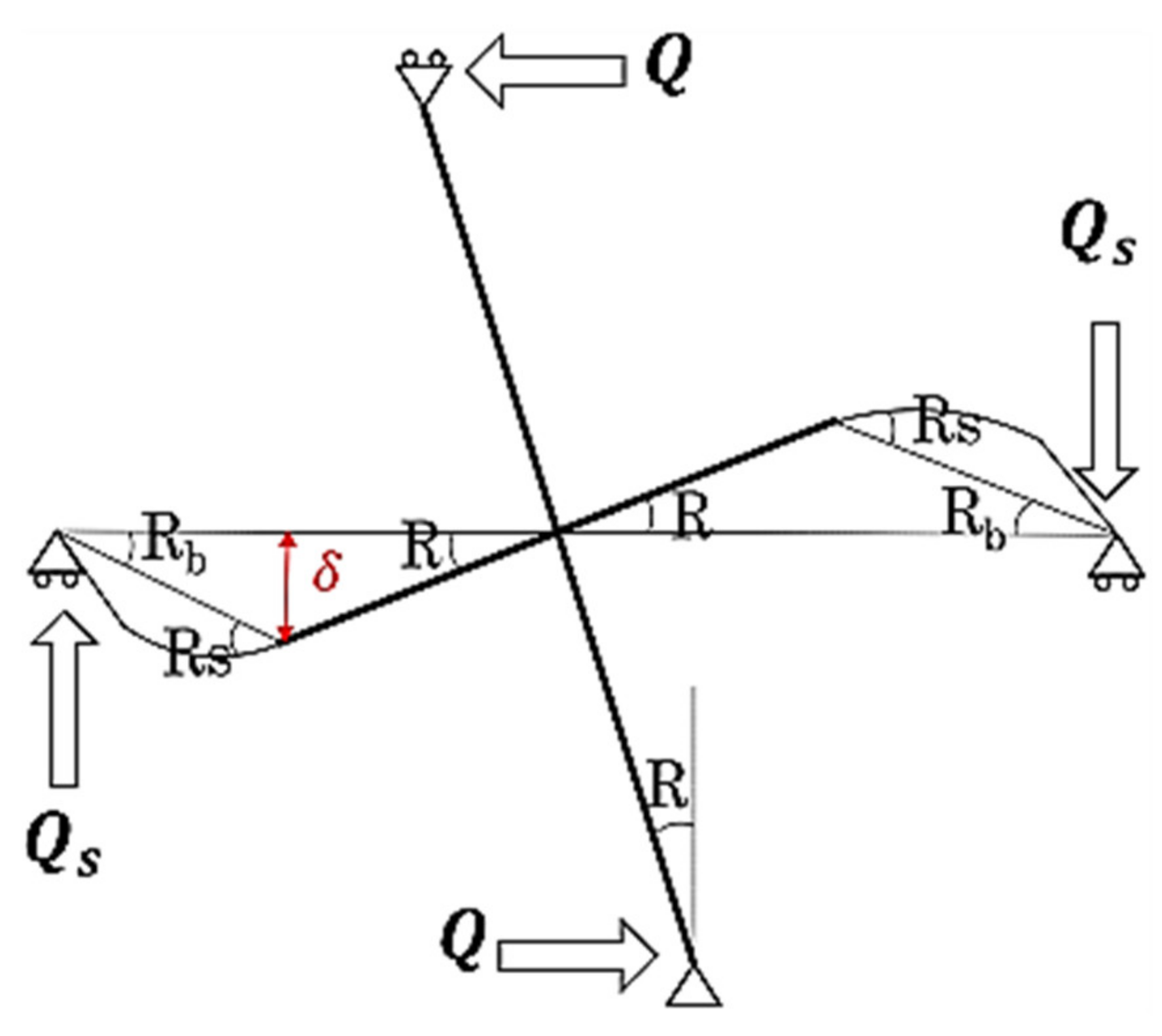
The dimension diagram of an individual wall-slab joint is shown in Figure 7a, while Figure 7b presents the deformation diagram when a lateral load named by $Q$ is subjected to the top of the bearing wall, in which the wall and joint portion are assumed as rigid bodies. $R$ is the rotational angle at the foot of the bearing wall while $R_s$ represents the rotational angle of the effective beam, and $L_s$ represents half the slab span length.

Thus, the rotational stiffness $K$ of the entire wall-slab joint can be expressed using the lateral load $Q$ and the rotational angle $R$ that represents the deformation angle of the strong bearing wall as given by Equation (1).

$$K=\frac{Q}{R}$$

(1)

Due to considerations of (i) the force supporting at the slab ends represented by $Q_s$, (ii) the rotational angle at the end of the effective beam noted using $R_s$, and (iii) the connection portion treated as a rigid region, the stiffness of the effective beam $K_s$ can be consequently expressed as given by Equation (2).

$$K_s=\frac{Q_s}{R_s}$$

(2)

Next, a relationship between $K$ and $K_s$ can be established using $Q$, $R$, $Q_s$, and $R_s$ as shown in Equation (3).

$$\frac{K}{K_s}=\frac{\frac{Q}{R}}{\frac{Q_s}{R_s}}=\frac{Q}{Q_s}\times \frac{R_s}{R}$$

(3)

Because there is a relationship between $Q$ and $Q_s$ concerning the equilibrium of moment around the joint core as shown in Equation (4), “$Q$/$Q_s$” can thus be expressed as shown in Equation (5) by rearranging Equation (4).

$$Q\cdot 2H=Q_s\times 2L_s$$

(4)

$$\frac{Q}{Q_s}=\frac{L_s}{H}$$

(5)

Additionally, “$R$/$R_s$” can be expressed using dimensions of wall and slab as given by Equation (6) due to the assumptions that the wall and the connection portion are treated as rigid bodies. It is noted that this equation is theoretically correct if the plastic hinge forms on the slab and is adjacent to the joint core.

$$\frac{R}{R_s}=\frac{L_2}{L_1}$$

(6)

Accordingly, by rearranging Equation (3) after substituting in “$\frac{Q}{Q_s}$” and “$\frac{R}{R_s}$” using Equations (5) and (6), respectively, “$\frac{K}{K_s}$” can be expressed by Equation (7) using values of the joint dimensions.

$$\frac{K}{K_s}=\frac{Q}{Q_s}\times \frac{R_s}{R}=\frac{L_s}{H}\times \frac{L_1}{L_2}=\frac{L_s{L}_1}{H{L}_2}$$

(7)

Thus, the effective beam stiffness $K_s$ can be obtained from $K$ by rearranging Equation (7) as shown in Equation (8).

$$K_s=\frac{H{L}_2}{L_s{L}_1}K$$

(8)

On the other hand, considering the thickness of the slab is $D$, $b_e$ can be as well expressed by Equation (9) if the required moment of inertia of area $I$ is known.

$$b_e=\frac{12I}{D^3}$$

(9)

Additionally, considering the effective beam as a normal beam element in which the flexible length of the beam is represented by $L_2$ (equals to “$L_s$-$L_1$”) as shown in Figure 7a, the rotational angle of the effective beam represented by $R_b$ can be consequently expressed by Equation (10).

$$R_b=\frac{L_2{}^2}{3EI}{Q}_b$$

(10)

Thus, assuming the stiffness of the effective beam as $K_b$, $K_b$ can be given by Equation (11) by rearranging Equation (10), where the moment of inertia of area $I$ has been given by Equation (12).

$$K_b=\frac{Q_b}{R_b}=\frac{3EI}{L_2{}^2}$$

(11)

$$I=\frac{b_e{D}^3}{12}$$

(12)

By substituting Equation (12) for $I$ into Equation (11), $K_b$ can be expressed by Equation (13).

$$K_b=\frac{3E}{L_2{}^2}\times \frac{b_e{D}^3}{12}$$

(13)

Because $K_b$ and $K_s$ are both representing the stiffness of the effective beam, indicating they should be equal, by setting $K_b$ expressed by Equation (13) to be equal with $K_s$ expressed by Equation (8) as shown in Equation (14), Equation (15) can thus be obtained. By rearranging Equation (15), the effective beam width $b_e$ is consequently expressed by Equation (16) using the joint stiffness $K$, component dimensions, and material features of the wall-slab joint.

$$K_s=K_b$$

(14)

$$\frac{H{L}_2}{L_s{L}_1}K=\frac{3E}{L_2{}^2}\times \frac{b_e{D}^3}{12}$$

(15)

$$b_e=\frac{4H{L}_2^3}{E{D}^3{L}_s{L}_1}K$$

(16)

Additionally, because $K$ can also be expressed by “$\frac{Q}{R}$”, where $Q$ represents the lateral force applied to the top of the wall while $R$ represents the rotational angle at the wall foot, Equation (16) can be rearranged to Equation (17).

$$b_e=\frac{4}{E{D}^3}\times \frac{L_2^3}{L_s{L}_1}\times \frac{QH}{R}$$

(17)

As a result, Equation (17) can be considered as the effective beam model to calculate the stiffness of an individual wall-slab joint under a lateral load $Q$ representing an earthquake excitation. It is noted that parts of “$\frac{4}{E{D}^3}$”, “$\frac{L_2^3}{L_s{L}_1}$”, and “$H$” can be obtained from model dimensions and material features, such as wall length, slab thickness, Young’s modulus of concrete, and others which can be obtained directly from design details. Only the $Q$ and $R$ which represent the applied lateral force and the rotational deformation angle of the joint are needed carefully discussed for applying this model in practical design.

Firstly, $R$ can be taken by the value of 0.05% due to the initial stiffness defined as the secant stiffness at 0.05% inter-story drift ratio (corresponding to 1/2000 rad inter-story deformation angle according to WRC Standard [3]). Therefore, Equation (17) can thus be rearranged to Equation (18) for predicting the effective beam width for the initial stiffness.

$$b_e=\frac{4}{E{D}^3}\times \frac{L_2^3}{L_s{L}_1}\times 2000\times QH$$

(18)

Next, for the applied lateral force $Q$, if the average shear stress distributing over its bearing wall cross-section plane of wall-slab joints when the required deformation value which represents the initial stage reaches, the value of $Q$ for Equation (18) can consequently be obtained by multiplying the average shear stress and its total cross-sectional area of the bearing wall. However, it is hard to accurately estimate the average shear stress distributed over the bearing wall, due to the shear stress of concrete at a very small deformation angle which is not stable nor identical for different situations. Therefore, to accurately estimate the value of force $Q$ applied to the bearing wall when the defined initial stage reaches, results of an experimental cyclic lateral loading test of thick wall-thick slab joints in TWTS structures conducted at Yamaguchi University in 2016 [6,7] are employed in this work. The measured lateral force applied on the top of the bearing wall at the inter-story drift ratio of 0.05% for specimens in their tests is used to provide a reasonable estimate of $Q$ at 0.05% inter-story drift ratio. These values from their experimental results are employed as criterion values and a correction coefficient is defined. Thus, by applying the criterion value and correction coefficient, an estimation of the crucial factor $Q$ for the effective beam width of initial stiffness prediction can be obtained. Detailed information of their experimental tests related to this work and the model processing using their resultant data are explained in the following sections.

4.3.2. Model Processing Using Experimental Tests Results

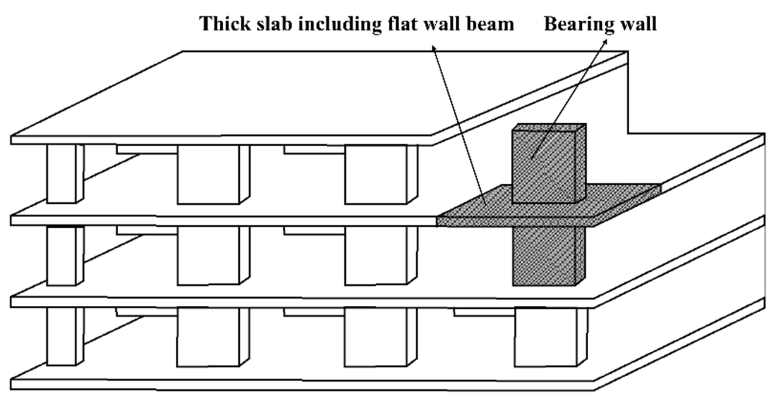
Four 1/2-scaled specimens of thick wall-thick slab joints were tested in Inai et al.’s experimental tests [6,7], from which three specimens are selected for the modeling processing in this work. Specimen 1 and 2 have slabs on both sides while Specimen 3 only has an individual slab on one side as shown in Figure 8 and Figure 9, respectively. The specimens have a uniform dimension for bearing wall (500 mm length, 1500 mm height, and 175 mm depth), flat slab (span length of 1500 mm and slab thickness of 175 mm), and the invisible beams that are concealed in the flat slab (length of 1500 mm equal to that of the slab, width of 350 mm, and depth of 175 mm). It is noticed that in their work, the bearing wall is not arranged symmetrically in the north-south direction, which is caused by the design consideration for the interior and exterior spaces (such as different reinforcement distribution for the indoor space and the balcony space). However, it is not affecting the flexural stiffness of solid components so that the discrepancy of the invisible beam component can be ignored for the stiffness calculation. Additionally, the properties and test results for concrete and steel materials in their test are summarized in

Table 1. Material test results of concrete [6,7].

Specimen	Compressive Strength (N/mm2)	Young’s Modulus (N/mm2)
1	38.50	31.90
2	36.80	32.20
3	37.50	31.10

.

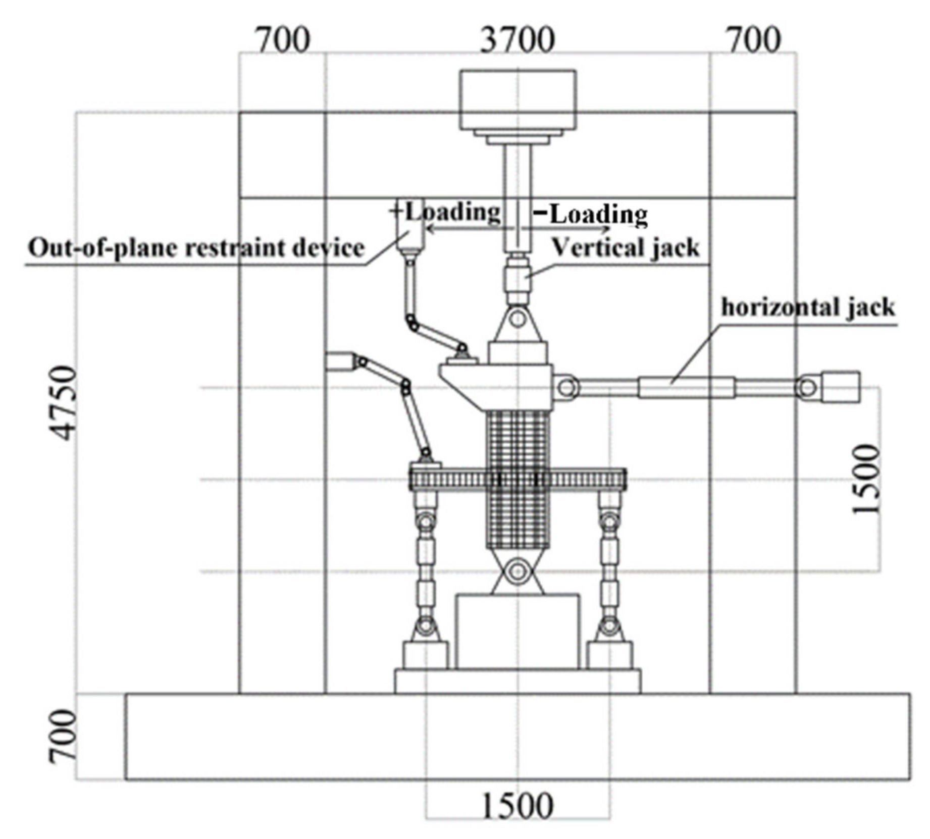
The fixity condition and test setup are shown in Figure 10. The bottom of the bearing wall was pin-supported on the strong ground to restrain the horizontal and vertical movements of the base, the top of the bearing wall was free where cyclic lateral loadings were applied, and both ends of the slab were roller-supported and restrained only in the vertical direction to simulate points of inflection.

Considering that the initial stiffness was defined as the secant stiffness at 0.05% inter-story drift ratio, the results from their experimental test of the lateral force at 0.05% drift ratio are defined as criterion values of the input lateral force $Q_0$, in which the subscript “0” represents the criterion value. Additionally, the specimen and material properties from their experimental test are as well considered as criterion values for further model processing, such as $A_{w0}$ for the wall cross-sectional area, $l_{w0}$ for the wall length, $t_{w0}$ for the wall thickness, and so on. Moreover, the initial stiffness $K_{b0}$ using Equation (1) and the effective beam width $b_{e0}$ using Equation (18) can be obtained as summarized in

Table 2. Application experimental test results to the proposed model.

Specimen	$\mathbf{The}\mathbf{applied}\mathbf{Lateral}\mathbf{Load}{\mathit{Q}}_0$ (kN)	$\mathbf{Initial}\mathbf{Rotational}\mathbf{Stiffness}{\mathit{K}}_{\mathit{b}0}$ (kN/rad)	$\mathbf{Effective}\mathbf{Beam}\mathbf{Width}{\mathit{b}}_{\mathit{e}0}$ (mm)	$\mathbf{The}\mathbf{Ratio}\mathbf{of}\mathbf{the}\mathbf{Effective}\mathbf{Beam}\mathbf{Width}\mathbf{Divided}\mathbf{by}\mathbf{the}\mathbf{Thickness}$ be/tw
1	24.10	48,200.00	563.86	3.20
2	24.10	48,200.00	558.61	3.20
3	18.60	37,200.00	446.37	2.60

. It can be noted that for wall-slab joints with only one-side slabs, the effective beam is 2.60 times the uniform thickness while for joints with both-side slabs, it should be taken by 3.20 times.

Thus, these values obtained from Inai et al.’s results can be used to estimate the lateral force for the effective beam width model at the initial stage. To estimate the lateral force $Q$ in Equation (18) using the criterion value $Q_0$, a correction coefficient that represents the relationship between the target value $Q$ and $Q_0$ is established in the following section.

First of all, ${\tilde{\tau }}_0$ representing the criterion value of the average shear stress distributed over the cross-sectional plane of the bearing wall at the 0.05% inter-story drift ratio is defined and it can be obtained using the criterion lateral force $Q_0$ divided by the total cross-sectional area of the bearing wall. Based on the measured results from Inai et al.’s experimental tests, ${\tilde{\tau }}_0$ equals 0.28 $N/m{m}^2$ for both-slab joints while 0.21 $N/m{m}^2$ for one-slab joints. Additionally, $A_{w0}$ represents the criterion value of the total cross-sectional area of the bearing wall, $l_{w0}$ represents the criterion value of the length of the bearing wall which equals 500 mm, and $t_{w0}$ is the criterion value of the thickness of the bearing wall which equals 175 mm. Thus, the criterion lateral force $Q_0$ can be expressed using the criterion average shear stress ${\tilde{\tau }}_0$, multiplying the criterion value of the total cross-sectional area of the bearing wall $A_{w0}$ (equaling to the product of $l_{w0}$ and $t_{w0}$) as shown in Equation (19):

$$Q_0={\tilde{\tau }}_0\times A_{w0}={\tilde{\tau }}_0\cdot l_{w0}\times t_{w0}$$

(19)

where,

${\tilde{\tau }}_0$: Criterion value of average shear stress distributed over the cross-sectional plane of the bearing wall.

$A_{w0}$: Criterion value of the total cross-sectional area of the bearing wall.

$l_{w0}$: Criterion value of the length of the bearing wall.

$t_{w0}$: Criterion value of the thickness of the bearing wall.

Similarly, for a target wall-slab joint, the lateral force $Q$ applied at the 0.05% inter-story drift ratio can be expressed using its average shear stress $\tilde{\tau }$ which is distributing over its bearing wall cross-section plane, multiplying its total cross-sectional area of the bearing wall $A_w$ (equaling to the product of $l_w$ and $t_w$) as shown in Equation (20):

$$Q=\tilde{\tau }\times A_w=\tilde{\tau }\times l_w\times t_w$$

(20)

where,

$\tilde{\tau }$: Average shear stress distributed over the cross-sectional plane of the bearing wall.

$A_w$: Total cross-sectional area of the bearing wall.

$l_w$: Length of the bearing wall.

$t_w$: Thickness of the bearing wall.

Thus, as given by Equation (21), a correction coefficient $\rho$ can be established by $Q$ shown in Equation (20) divided by $Q_0$ shown in Equation (19). It is noted that only if the dimensions of the bearing wall is designed identical to that in Inai et al.’s models, the correction coefficient $\rho$ is thus as well the correction coefficient between the average shear stress $\tilde{\tau }$ and the criterion average shear stress ${\tilde{\tau }}_0$.

$$\rho =\frac{Q}{Q_0}=\frac{\tilde{\tau }\times l_w\times t_w}{{\tilde{\tau }}_0\times l_{w0}\times t_{w0}}$$

(21)

As shown in Figure 11, the supporting force applied to the slab end can be defined as $Q_s$ and has a relationship with $Q$ as given by Equation (22).

$$Q\times 2H=Q_s\times 2L_s$$

(22)

Concerning the geometric relationship, the rotational angle at the slab end $R_s$ can be expressed by $R_b$ plus the rotational angle of the bearing wall $R$, as given by Equation (23).

$$R_s=R_b+R$$

(23)

Assuming the displacement of the end of the rigid connection area is $\delta$, $\delta$ can be expressed by multiplying the rotational angle and the flexural length for both sides as shown in Equation (24) and Figure 11, where the definition of flexural length $L_1$ and $L_2$ are explained in Figure 7.

$$\delta =R_b\times L_2=R\times L_1$$

(24)

Next, by substituting Equation (24) for $R_b$ into Equation (23), $R_s$ can thus be expressed using the rotational angle $R$ and joint dimensions as given by Equation (25).

$$R_s=\frac{L_s}{L_2}\times R$$

(25)

The slab stiffness can be expressed in two ways: (i) $Q_s$ divided by $R_s$ shown in Equation (2), and (ii) $3EI$ divided by squared slab flexural length $L_2$ as given by Equation (26), respectively. By equalling these two formulas, $Q_s$ can thus be expressed as shown in Equation (27).

$$K_s=\frac{3EI}{L_2{}^2}$$

(26)

$$Q_s=\frac{3EI}{L_2{}^2}\times R_s$$

(27)

Then, by substituting Equation (25) for $R_s$ into the Equation (27), $Q_s$ can accordingly be expressed by $R$ as shown in Equation (28).

$$Q_s=\frac{3EI{L}_s}{L_2{}^3}\times R$$

(28)

Next, substituting Equation (28) for $Q_s$ into Equation (23), and considering $L_2$ equals “$L_s-L_1$”, a relationship between $Q$ and $R$ can be established as given by Equation (29).

$$Q=\frac{3EI{L}_s{}^2}{H{\left(L_s-L_1\right)}^3}\times R=3EI\times \frac{L_s{}^2}{H{\left(L_s-L_1\right)}^3}\times R$$

(29)

Using this formula, the criterion value $Q_0$ can consequently be expressed as given by Equation (30).

$$Q_0=3E_0{I}_0\times \frac{L_{s0}{}^2}{H_0{\left(L_{s0}-L_{10}\right)}^3}\times R_0$$

(30)

Thus, a correction coefficient $\rho ,$ representing the ratio between the unknown value $Q$ for a target wall-slab joint and the criterion value $Q_0,$ can be established using Equation (29) divided by Equation (30) as given by Equation (31).

$$\rho =\frac{Q}{Q_0}=\frac{3EI\times \frac{L_s{}^2}{H{\left(L_s-L_1\right)}^3}\times R}{3E_0{I}_0\times \frac{L_{s0}{}^2}{H_0{\left(L_{s0}-L_{10}\right)}^3}\times R_0}$$

(31)

Because the initial stiffness is defined as 0.05% inter-story drift ratio in this study, “$R=R_0=0.05\%$” can be substituted into Equation (31). Thus, Equation (31) is simplified to Equation (32) by eliminating $R$ and $R_0$. Generally, the applied lateral force changes and the stiffness reduction needs to be considered as the deformation process, which leads to a reduction of the effective beam width, while when the deformation is small enough, the deformation change and the stiffness reduction can be ignored so that the stiffness can be seen as a constant value. Thus, the applied lateral force can be consequently considered stable as a constant. Based on these considerations, it is noted that the $R$ and $R_0$ are set as 1/2000 rad for the initial stage in this work because the deformation angle is relatively small enough at the initial stage.

$$\rho =\frac{3EI\times \frac{L_s{}^2}{H{\left(L_s-L_1\right)}^3}}{3E_0{I}_0\times \frac{L_{s0}{}^2}{H_0{\left(L_{s0}-L_{10}\right)}^3}}$$

(32)

Additionally, the moment of inertia of area $I$ and $I_0$ in Equation (32) are assumed by 3.20 times the wall thickness for joints with both-side slabs and 2.60 times the wall thickness for joints with one-side slab according to measured results from the experimental data as shown in Table 2 previously.

Thus, the unknown value $Q$ can be estimated using the criterion value $Q_0$ and the correction coefficient $\rho$ is given by Equation (33).

$$Q=\rho \times Q_0$$

(33)

As a result, an estimated value of the lateral force at the initial stage obtained using Equations (32) and (33) can thus be applied to Equation (18) for predicting the effective beam width for the initial stiffness. This analytical-based, effective beam width estimation is derived for practical designing the wall-slab joints in TWTS structures. The proposed effective beam-width model provides a relatively accurate and convenient estimation for determining the slab design by limiting the minimum value on the width. Additionally, using this proposed model, it can as well model the entire wall-slab joints as a wall-beam frame, which leads to a simplified two-dimension frame analysis by substituting the slab components using the proposed effective beam.

4.3.3. Discussions on Influencing Factors

In the proposed model of the effective beam width for the initial stiffness, various features of the joint including the configuration dimensions and material properties, such as the concrete elastic modulus $E$, the thickness of the slab $D$, half of the wall height $H$, half of the wall height $L_1$, half of the slab span length $L_s$, and the flexural length of the slab $L_2,$ has been considered. The influence of two main factors, the wall height “$H$”, the wall length “$L_1$”, and the slab span length of “$L_s$” on the effective beam width prediction is discussed in this section.

Considering a situation in which except for the parameter of “$H$”, other features of the wall-slab joints are kept identical to discuss the influence of “$H$”, due to the strong bearing wall being assumed as a rigid body, the rotational angles generated for the slab ends are usually equaling to the value at an identical deformation angle occurring around the bearing wall footing at the initial stage. In other words, the input moment transferred over the effective beam is identical for cases with different values of $H$. Thus, the value of “$QH$” is consequently considered unchanged for different wall-slab joint models with different “$H$”. As a result, it can be known that if only the value of “$H$” is changing while other variables are kept identical, the value of $b_e$ predicted using Equation (18) is a constant. However, it should be noticed that the model was developed by assuming the bearing wall was a rigid body, which was reasonable considering calculation simplification but not completely true in reality. In actual structures, initial and growing cracks, shrinkage, creeps, or other damages occur in the bearing wall, which could make the stiffness of the bearing wall reduce, can bring slight influences on the value of “$QH$” and leads to the value of “$QH$” not keeping a constant and showing a slight change. As a result, in the situation that only “$H$” changes, it can be considered that the effective beam width is predicted identical at the initial stage with sufficiently small deformation, based on which slight influences can be ignored.

Due to $L_2$ equals to “$L_s-L_1$”, Equation (18) can also be expressed by Equation (34).

$$b_e=\frac{4}{E{D}^3}\times \frac{{\left(L_s-L_1\right)}^3}{L_s{L}_1}\times 2000\cdot QH$$

(34)

It can be known that $b_e$ is disproportionate to the thickness of the slab “$D$”, while for the group of “$\frac{{\left(L_s-L_1\right)}^3}{L_s{L}_1}$”, more discussions are needed to figure out how these two parameters, $L_s$ and $L_1$, influence the value of $b_e$. In the group “$\frac{{\left(L_s-L_1\right)}^3}{L_s{L}_1}$”, as the value of wall length $L_1$ increases, the part of “$L_s-L_1$” representing the flexural length of the effective beam decreases, which leads to a reduction of the calculation value of $b_e$. Thus, it can be indicated that the length of the bearing wall is as well disproportionate to the value of $b_e$. On the other hand, in the situation that the slab span length $L_s$ increases, both of “$L_s-L_1$” as well as “$L_s{L}_1$” increases, which is not clear to determine whether the value of “$\frac{{\left(L_s-L_1\right)}^3}{L_s{L}_1}$” increases or decreases. Therefore, for the parameter of the span length of the slab $L_s$, further investigations are needed in future work.

5. Comparison with Current Code Equations

The current standard for reinforced concrete structures provisions [2] recommend a calculation equation for T-shaped structural components in which the additional effect of slabs needed to be considered use the formula given by Equation (35) and illustrated in Figure 12:

$$b_a=\left\{\begin{array}{cc}\hfill \left(0.5-0.6\frac{a}{l}\right)a,& \frac{a}{l}<0.5\hfill \\ \hfill 0.1l,& \frac{a}{l}\ge 0.5\hfill \end{array}\right.$$

(35)

where,

$B$: Total effective beam width corresponding to $b_e$ in this work.

$b_a$: Effective proportion of slab contributing to the effective beam.

$a$: Distance between two side surfaces of two adjacent T-shaped structural components.

$b$: Thickness of the vertical supporting structural component corresponding to the thickness of the bearing wall in this work.

$l$: Span length of frames corresponding to the slab span length in this work.

Thus, a comparison of the calculated value of effective beam width for the three specimens from Inai et al.’s experimental test [6,7] using the proposed model and the code equations are summarized in

Table 3. Comparison of the effective beam width.

Specimen	Code Formula Calculations (mm)	Proposed Model Calculations (mm)
1	475.00	563.86
2	475.00	558.61
3	325.00	446.37

.

For these specimens, a is 1000 mm while l is 1500 mm for code equations so that it can be obtained “$\frac{a}{l}$” equals 0.67 which is greater than 0.5. The effective proportion of slab contributing to the effective beam $b_a$ is consequently calculated equaling 150 mm using Equation (35). Therefore, the effective beam width $B$ based on the code equations is predicted as 475 mm for both-slab joints (Specimen 1 and 2) and 325 mm for one-slab joint (Specimen 3). However, it has been known, as shown in Table 3, that the effective beam width $b_a$ obtained from the results of the experimental test are 563.86 mm, 558.61 mm, and 446.37 mm for these specimens, respectively. The values calculated using Equation (35) are lower than those obtained from experimental data either for both or one-slab joints. Thus, it can be known that the equations employed in the current code underestimate and are not appropriate to evaluate the effective beam width for initial stiffness at the elastic stage, which might result in giving a higher initial deformation angle prediction which is larger than 1/2000 rad at the elastic stage and consequently, large cracks or shear failure may wrongly be predicted for the design target deformation angle of 1/200 rad (0.05% drift ratio), finally. In contrast, since the proposed prediction model is analytically established from the actual experimental test setup, which can give an appropriate prediction of the effective beam width, the initial stiffness of the wall-slab joints in TWTS structures can be evaluated by the proposed prediction model with more accuracy and higher efficiency than the current code equations.

6. Suggestions for Practical Design and Limitations

Based on the results obtained from this work, the following design recommendations on the wall-slab joints in TWTS structures can be drawn.

Firstly, a design procedure for the application of the effective beam width prediction model has been suggested.

Step 1: Determine the correction coefficient $\rho$ using Equation (32).

Step 2: Estimate the unknown value of lateral force $Q$ carried by the target wall-slab joint at the top of the bearing wall using the correction coefficient $\rho$ and Equation (33).

Step 3: Apply $Q$ into Equation (18) to obtain the prediction value of the effective beam width $b_e$.

Step 4: By using the effective beam width $b_e$, the initial stiffness of the wall-slab joint can thus be predicted.

However, because of the assumptions and estimations for developing this model, the following limitations are needed to be noticed for practical design:

• Only if this assumption that the bearing wall and the wall-slab connection portion being considered as rigid bodies is reasonably true, the proposed prediction model shown in Equation (18) is applicable.
• Using the proposed model, the effective beam width for the initial rotational stiffness can be accurately predicted if the applied lateral force at the 0.05% inter-story drift ratio is known. Nonetheless, it is difficult to obtain the accurate value of the lateral force at the elastic stage. To solve this problem, a correction coefficient employing the experimental results from the literature is used and gives a reasonable estimation for the practical design. However, as a new type of structural system, limited experimental tests and not sufficient studies have been conducted, which makes the lateral force estimation considered only applicable for wall-slab joints similar to the specimens from the experimental test referred to in this work. Thus, further research is needed to investigate the effective beam width for the initial stiffness in a larger scope.

7. Conclusions

In this study, a prediction model was developed for the effective beam width for the initial stiffness of the wall-slab joints in TWTS structures based on the EBWM concept. Additionally, by applying experimental data from the literature, a practical application procedure using the proposed model is as well suggested. Thus, the following conclusions can be drawn from this work:

(i)

The prediction model of the effective beam width for the initial stiffness which is defined as the stiffness at 0.05% inter-story drift ratio of wall-slab joints in TWTS structures has been proposed as shown in Equation (18).

(ii)

By applying the results from an experimental test, a correction coefficient $\rho$ to estimate the unknown value of the lateral force for the initial stiffness has as well been proposed as shown in Equation (32).

(iii)

Using the proposed analytical prediction model, a practical design procedure has been suggested.

(iv)

The effects of parameters that are involved in the prediction model, such as the height and length of bearing wall, and the span length of slab on effective beam width have been discussed.

(v)

Due to several assumptions being made for the model processing, the applicable scope of this proposed model has been carefully defined. Moreover, one of the indexes of this model is estimated using limited experimental data from the literature. This model can give a good prediction for similar target specimens in practical design, but there is a need to perform further experimental tests to enlarge the usage scope of the proposed model.

Finally, it should be noted that the prediction model of the effective beam width for the initial stiffness of wall-slab joints in TWTS structures proposed in this study is more engineering-oriented, by which the seismic performance design and assessment can be achieved in a reasonable and simplified manner.

References

1. Inoue, Y.; Teshigawara, M. Guidelines for Structural Performance Evaluation of Reinforced Concrete Boxed Wall-Buildings (Draft). Concr. J. 2009, 47, 3–10. [Google Scholar] [CrossRef]
2. AIJ. Standard for Structural Calculation of Reinforced Concrete Structures; Architectural Institute of Japan: Tokyo, Japan, 2018. [Google Scholar]
3. AIJ. The Standard for Structural Design of Reinforced Concrete Boxed-Shaped Wall Structures; Architectural Institute of Japan: Tokyo, Japan, 2018. [Google Scholar]
4. AIJ. Preliminary Reconnaissance Report of the 2011 Tohoku-Chiho Taiheiyo-Oki Earthquake; Architectural Institute of Japan: Tokyo, Japan, 2011. [Google Scholar]
5. AIJ. Report on the Damage Investigation of the 2016 Kumamoto Earthquake; Architectural Institute of Japan: Tokyo, Japan, 2018. [Google Scholar]
6. Inai, E.; Kawata, Y.; Akita, T.; Imagawa, N. Loading tests in the in-plain direction of wall-slab joints in box-shaped thick slab and thick wall structures (Part 1–5). Proceedings of Annual Research Meeting Chugoku Chapter. Archit. Inst. Jpn. (AIJ) 2017, 40, 247–266. [Google Scholar]
7. Inai, E.; Kawata, Y.; Akita, T.; Imagawa, N.; Ikeda, H. Seismic behavior in the in-plain direction of wall-slab joints of reinforced concrete box-shaped thick slab-thick wall structures (Part 1–4). Summaries of technical papers of annual meeting. Archit. Inst. Jpn. 2017, 2017, 881–887. [Google Scholar]
8. Tsuboi, Y.; Kawaguchi, M. On Earthquake Resistant Design of Flat Slabs and Concrete Shell Structures. In Proceedings of the Second World Conference on Earthquake Engineering, Tokyo and Kyoto, Japan, 11–18 July 1960; Volume III, pp. 1693–1708. [Google Scholar]
9. Pecknold, D.A. Slab Effective Width for Equivalent Frame Analysis. ACI Struct. J. 1975, 72, 135–137. [Google Scholar]
10. Vanderbilt, M.D.; Corley, W.G. Frame Analysis of Concrete Buildings. Concr. Int. Des. Constr. 1983, 5, 12. [Google Scholar]
11. Luo, Y.H.; Durrani, A.J.; Conte, J.P. Equivalent Frame Analysis of Flat-Plate Buildings for Seismic loading. J. Struct. Eng. 1994, 120, 2137–2155. [Google Scholar] [CrossRef]
12. Luo, Y.H.; Durrani, A.J. Equivalent Beam Model for Flat-Slab Buildings Part I: Interior Connections. ACI Struct. J. 1995, 92, 115–124. [Google Scholar]
13. Luo, Y.H.; Durrani, A.J. Equivalent Beam Model for Flat-Slab Buildings Part II: Exterior Connections: Interior Connections. ACI Struct. J. 1995, 92, 250–257. [Google Scholar]
14. Hwang, S.; Moehle, J.P. Models for Laterally Loaded Slab-Column Frames. ACI Struct. J. 2000, 97, 345–352. [Google Scholar]
15. Dovich, L.M.; Wight, J.K. Effective slab width model for seismic analysis of flat slab frames. ACI Struct. J. 2005, 102, 868–875. [Google Scholar]
Figure 1. An example frame of WRC structures.
Applsci 12 04600 g001
Figure 2. Thick wall-thick slab building view.
Applsci 12 04600 g002
Figure 3. Development of thick wall-thick slab structures.
Applsci 12 04600 g003
Figure 4. Relation of initial stiffness and maximum inter-story deformation angle.
Applsci 12 04600 g004
Figure 5. Definition of EBWM.
Applsci 12 04600 g005
Figure 6. Calculation flow chart for the effective beam width b e .
Applsci 12 04600 g006
Figure 7. The effective beam at the wall-slab joints in TWTS structures.
Applsci 12 04600 g007
Figure 8. Design details for both-slab specimen (dimensions in mm) [6,7].
Applsci 12 04600 g008
Figure 9. Design details for one-slab specimen (dimensions in mm) [6,7].
Applsci 12 04600 g009
Figure 10. Loading arrangement [6,7].
Applsci 12 04600 g010
Figure 11. Calculation diagram.
Applsci 12 04600 g011
Figure 12. Effective beam width prediction in the current RC Standard.
Applsci 12 04600 g012