Article

Whitening CNN-Based Rotor System Fault Diagnosis Model Features

1
Department of Mechanical Engineering, Aalto University, 02150 Espoo, Finland
2
Control Engineering, Environmental and Chemical Engineering, University of Oulu, 90014 Oulu, Finland
3
Kongsberg Maritime Finland Oy, 26101 Rauma, Finland
4
Department of Electrical Engineering and Automation, Aalto University, 02150 Espoo, Finland
*
Author to whom correspondence should be addressed.
Appl. Sci. 2022, 12(9), 4411; https://doi.org/10.3390/app12094411
Submission received: 5 April 2022 / Revised: 20 April 2022 / Accepted: 25 April 2022 / Published: 27 April 2022
(This article belongs to the Special Issue Disruptive Trends in Automation Technology)

Abstract

:
Intelligent fault diagnosis (IFD) models have the potential to increase the level of automation and the diagnosis accuracy of machine condition monitoring systems. Many of the latest IFD models rely on convolutional layers for feature extraction from vibration data. The majority of these models employ batch normalisation (BN) for centring and scaling the input for each neuron. This study includes a novel examination of a competitive approach for layer input normalisation in the scope of fault diagnosis. Network deconvolution (ND) is a technique that further decorrelates the layer inputs reducing redundancy among the learned features. Both normalisation techniques are implemented on three common 1D-CNN-based fault diagnosis models. The models with ND mostly outperform the baseline models with BN in three experiments concerning fault datasets from two different rotor systems. Furthermore, the models with ND significantly outperform the baseline models with BN in the common CWRU bearing fault tests with load domain shifts, if the data from drive-end and fan-end sensors are employed. The results show that whitened features can improve the performance of CNN-based fault diagnosis models.

1. Introduction

A malfunctioning rotating system is a common concern across a multitude of industries in the modern world. A malfunction in a rotating system can be caused by a number of reasons such as faulty bearings, broken shafts or worn gears. Typically, these faults increase the harmful vibration of the system by exciting the rotating parts on a per revolution basis. Often these excitations that alter the vibration profile of the system can be observed from measurements conducted with vibration sensors such as accelerometers.
Vibration based fault diagnosis for rotating systems has been developed for decades [1]. Most developed methods can be described as two step processes of feature extraction and fault recognition [2]. Features can be extracted from vibration data with a set of signal processing techniques in the time domain, the frequency domain and the time-frequency domain [3]. Typically, the features most sensitive to various faults are then exploited in fault recognition. Some of the studied fault recognition models employing traditional machine learning rely on, for example, random forests [4], support vector machines [5] and shallow neural networks [6]. Despite the successful results related to these techniques, they still suffer from a few disadvantages. Designing the signal processing techniques for feature extraction requires manual labour and often task-specific feature selection. Furthermore, the learning capacity of the models limits their performance if many non-linear relations between the input space and the fault label space are required.
Currently, deep learning (DL) seems like a promising solution for the challenges related to the other machine learning (ML) related fault diagnosis techniques. Deep learning requires no manual feature extraction nor sophisticated signal processing techniques, for it can be utilized to process the raw vibration data directly. The advantage of DL algorithms originates from their capacity to learn hierarchical and non-linear features autonomously between the raw data and the fault label space [7]. This implies that both steps, the feature extraction and the fault recognition can be simultaneously optimised and combined under one deep learning model. Furthermore, some studies have indicated that features acquired with deep learning increase the machine fault classification accuracy and noise tolerance when compared to features acquired with signal processing tools [8,9].
These advantages have attracted a growing amount of research interest toward deep learning based fault diagnosis [1,10,11]. Many deep learning architectures, such as deep-belief networks (DBN) [12], autoencoders (AE) [9] and recurrent neural networks (RNN) [13] have been proposed for anomaly detection and fault diagnosis tasks. Despite these impressive results, learning the rich features required for fault recognition is difficult. Fortunately, many works have shown that convolutional neural networks (CNN) are effective in extracting features from vibration data [1,10,14]. For example, a number of studies have shown that 1D-CNNs can diagnose faults from time-series data [15,16,17,18]. Furthermore, a number of studies have also demonstrated that CNNs can effectively diagnose faults from the vibration frequency spectrum [19,20,21]. In addition, some studies have demonstrated the efficiency of 2D-CNNs for diagnosing the faults from time-frequency spectrograms [19,22]. Furthermore, CNN-based fault diagnosis models seem to be at the core of the most recent research branch of fault diagnosis concerning transfer learning [23,24,25]. Although deep learning based fault diagnosis models have been extensively studied and the focus seems to be shifting towards transfer learning, the techniques improving the feature extraction of the current models are still relevant.
Many of the recent CNN-based state-of-the-art deep learning algorithms for fault diagnosis rely on batch-normalisation (BN) [15,16,17]. BN efficiently accelerates the model convergence and improves model generalisation [26,27]. In essence, this standardisation method centres and scales the layer activations based on the mini-batch statistics [26]. Centring and scaling each layer activation per mini-batch effectively stabilises the gradient distribution for each corresponding weight [27]. Stabilised gradient distribution increases the consistency of the gradient descent. However, BN can be considered an incomplete normalisation method, since its design includes a compromise that separates it from whitening [26]. In addition to centering and scaling, whitening includes decorrelation, which has been argued to simplify the optimisation of the model weights by making the adjacent weights independent [28]. Decorrelation has been excluded from BN due to the heavy toll it introduces to the computation [26]. Fortunately, recent studies have shown how to implement full whitening of the activations without excessive computational cost. These studies have also shown that whitening improves the learning results over BN [29,30,31].
Despite the promising results regarding feature whitening techniques, CNN-based fault diagnosis models still mostly rely on BN. This study shows how whitening the layer activations improves the current state-of-the-art 1D-CNN-based algorithms for machine fault diagnosis. The novel experiments employ three previously published fault diagnosis models. These commonly known models are Ince’s model [32], WDCNN [15] and SRDCNN [18]. The experiments reveal the fault diagnosis accuracies of these baseline models in parallel with corresponding models employing a whitening normalisation technique instead of BN. The whitening technique is adapted from an earlier study showing that decorrelating layer inputs channel-wise and pixel-wise consistently improved 2D-CNNbased model performance and training convergence on image data [31]. This “network deconvolution” (ND) operation, developed in [31], is further adjusted and integrated with the three 1D-CNN-based fault diagnosis models for time series data in this study. The experiments of this work complement the previously reported results with ND performance in 1D-CNN-based models. The three experiments in this study employ two vibration datasets acquired from different rotor systems. The first dataset is the thoroughly studied bearing fault dataset produced by Case Western Reserve University [33]. The second dataset consists of vibration data from three azimuth thrusters before and after bearing and gear related faults were noticed. Each experiment shows that models with whitened features achieve high performance. More specifically, the models with whitened features achieve mostly better or significantly better diagnosis accuracies compared to the baseline models in the three experiments.

2. CNNs and Normalization Layers

Convolutional neural networks (CNNs) typically consist of convolutional layers, pooling layers, normalisation layers and a few fully connected layers. In vibration-based fault classification, the final fully-connected layer can be considered as the classifier in the fault recognition step. The other fully-connected layers, convolutional layers, normalisation, and pooling layers are used for the feature extraction step.

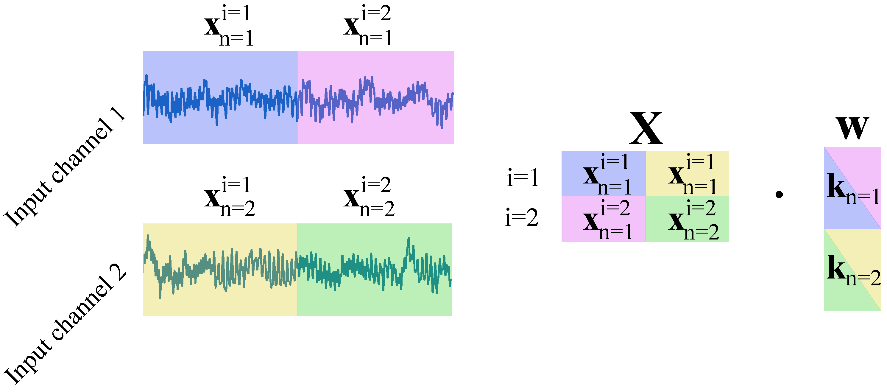
2.1. 1D Convolutional Layer

1D convolutional layers consist of filters computing cross-correlations over local areas of the input. Each filter consisting of N kernels with M weights computes an output value for a local area that consists of N × M values, where N denotes the number of channels e.g., different vibration sensors at the first layer and M denotes the length of the local area e.g., time steps. The filters process the local areas subsequently along the length axis with the same set of weights. Equation (1) shows this cross-correlation computation for a given local area:
y j l , i = n = 0 N k j , n l x n l , i + b j , n l
where y j l , i denotes the i-th local area output value of j-th filter on the layer l, k j , n l is the kernel for n-th channel of j-th filter on the layer l, x n l , i is the n-th channel of the i-th local area, ∗ denotes the dot product and b j , n l is the bias term of the kernel n of filter j on layer l. To conclude, the output value y j l , i is the sum of the dot-products between the kernels and the local areas computed at each corresponding input channel n. This computation is commonly referred to as the depth-wise convolution.
The computation at a given convolutional layer can be formulated as matrix multiplication Xw . With one dimensional data and a single input channel, for example, time series data from a single sensor at the first layer, the rows in matrix X would correspond to each local area x 1 1 , i and w corresponds to a column vector of the weights in the only kernel k j , 1 1 of the filter j. Typically, there are multiple input channels to each convolutional layer, and the number of kernels in a convolutional layer filter equals the number of input channels to that layer. The local areas x n l , i of the latter input channels are concatenated to the transformed data matrix X , so that each local area x n i , corresponding to the i-th convolution, are on the same row. Similarly, the weights of each kernel k n for all channels n are vertically concatenated to the column vector w . This transformation of input data to matrix X is similar to the commonly known im2col transformation with the difference that time series data is one-dimensional. The transformation is visualised in Figure 1.

2.2. Pooling Layer and ReLU Activation

Pooling layers efficiently reduce the model complexity and redundant information passed between the layers in CNNs. Each pooling layer consists of kernels that slide through the input array similar to the convolution layer kernels. Pooling layers rely on sub-sampling each local area under the kernels’ receptive field. The most common pooling layers are the max-pooling and the average-pooling layer. Max-pooling has been shown to consistently outperform average pooling [34]. A max-pooling layer compresses the signals between layers by concatenating the maximum values of each local area for every channel separately. Equation (2) demonstrates the max-pooling operation:
y ^ j l , k = m a x ( y j l , k )
where y j l , k denotes the values under the max-pooling kernel receptive field from the k-th local area of the j-th channel between convolutional layers l and l + 1 , and y ^ j l , k is the corresponding maximum value.
Typically between consequent cross-correlation computations, the output values are processed with a non-linear activation function, such as the rectified linear unit (ReLU) shown in Equation (3). The processed output values x j l + 1 , i can then be passed forward to the next layer l + 1 .
x j l + 1 , i = R e L U ( y j l , i ) = m a x ( 0 , y j l , i )

2.3. Batch Normalisation

Batch normalisation (BN) layers are additional layers that fix the activation distributions. This technique reduces the effect of internal covariate shift, a phenomenon hindering stochastic gradient descent optimisation [26]. Internal covariate shift can be described as a drastic change in the activation distributions due to the changed network parameters. BN normalises each activation separately with activation mean μ b and variance σ b 2 estimated from the mini-batch statistics. Furthermore, BN learns an additional set of scale γ and shifts β parameters by backpropagation. The computations related to BN are shown in Formulas (4)–(7).
μ b 1 m i = 1 m x i
σ b 2 1 m i = 1 m ( x i μ b ) 2
x ^ i x i μ b σ b 2 + ϵ
y i γ x ^ i + β
In Formulas (4)–(6), x i denotes the i-th convolution layer output values in a batch, i.e., x i = y j l , i as in Equation (1). More explicitly, x i X = [ x 1 m ] , where X is the batch with m convolution layer activations y j l , i . Alternatively, BN can operate on the activation values given by the ReLU-activation function in Equation (3). In Formulas (4) and (5), the mean μ b and the variance σ b 2 are computed from the distribution of the corresponding output values in the batch. Formula (6) shows the normalisation computation, where x ^ i is the normalised output, and ϵ is a small constant introduced for numerical stability. In Formula (7), y i is the BN layer output and γ and β are weights for scaling and shifting activations, optimised with backpropagation. Furthermore, during training the moving averages of μ b and σ b 2 are collected and utilised during testing.

2.4. From BN to Whitening Features

Image data may contain correlating data between nearby pixels and channels. For example, the pixels nearby a blurry object in an image correlate spatially. In addition, a grey object in an RGB image results in channel-wise correlation, since the RGB values are close to equal in the grey pixels. Machine vibration data may contain a similar correlation. For example, nearby sensors likely collect similar vibration patterns. Such data can hamper the optimisation process by inducing a correlation between the features learned by the neural network. Moreover, correlated features have been deemed problematic for neural network optimisation in the past [28].
Although BN has been shown to be effective in numerous state-of-the-art works [35,36,37,38], it merely scales and shifts the activations. BN was not designed to decorrelate the features due to the expense of computing the inverse square root of the activation covariance matrix and the corresponding derivatives. Nevertheless, several normalisation techniques that also decorrelate features have been proposed. These techniques typically seek better optimisation results by whitening the activations directly. Activations can be whitened for example according to the population statistics [39,40]. However, the estimation of the population statistics is hindered by the computational constraints and the changes to the activation distributions caused by the weight updates during optimisation [27]. Fortunately, these problems can be avoided by whitening the activations based on the mini-batch statistics. Such techniques are, for example, decorrelated batch normalisation (DBN) [30], IterNorm [41] and network deconvolution [31]. These three techniques first estimate the covariance matrix of the activations in the batch, as shown in Equation (8). In Equation (8), X R C × N is the activation matrix with C channels and N samples, and μ R C is the mean of the N activations in the batch. The batch of activations is then whitened with the inverse square root of the covariance matrix, i.e., the whitening matrix, and the batch mean, as shown in Equation (9). DBN has a slight disadvantage since it computes the whitening matrix with eigenvalue decomposition. IterNorm was proposed to solve the computational problems of DBN. IterNorm approximates the inverse square root of the whitening matrix with Newton’s iteration. Network Deconvolution is similar to IterNorm. However, it employs coupled Newton-Schulz iteration, which was shown both a quick and stable approximation technique for the whitening matrix [31].
Cov = 1 N ( X μ ) T ( X μ )
X ˜ = ( X μ ) Cov 1 2

3. Proposed Improvement for Fault Diagnosis Models

This study seeks to improve the current state-of-the-art CNN-based techniques for diagnosing faults from raw vibration data. The experiments in this study adapt three reportedly highly performing 1D-CNN models, remove all BN functions and normalise the layer inputs with ND instead. The study then evaluates the original models employing BN in parallel with the corresponding models employing ND. The baseline models are known as Ince’s model [32], the stacked residual dilated convolutional neural network (SRDCNN) [18] and the Deep Convolutional Neural Networks with Wide First-layer Kernels (WDCNN) [15]. Although numerous other fault diagnosis models exist, these were chosen due to their simple and effective architectures. For example, WDCNN has been shown to produce the best bearing fault diagnosis results with slight modifications as an ensemble [16] and with an additional RNN-path [17]. However, the contrast in the results between models employing ND and BN can be sufficiently shown with these models without additional modifications.
This section is divided into three parts. Section 3.1 visits briefly the baseline model architectures. Then, Section 3.2 describes the ND practical implementation details. Finally, some general training algorithmic design choices are presented in Section 3.3.

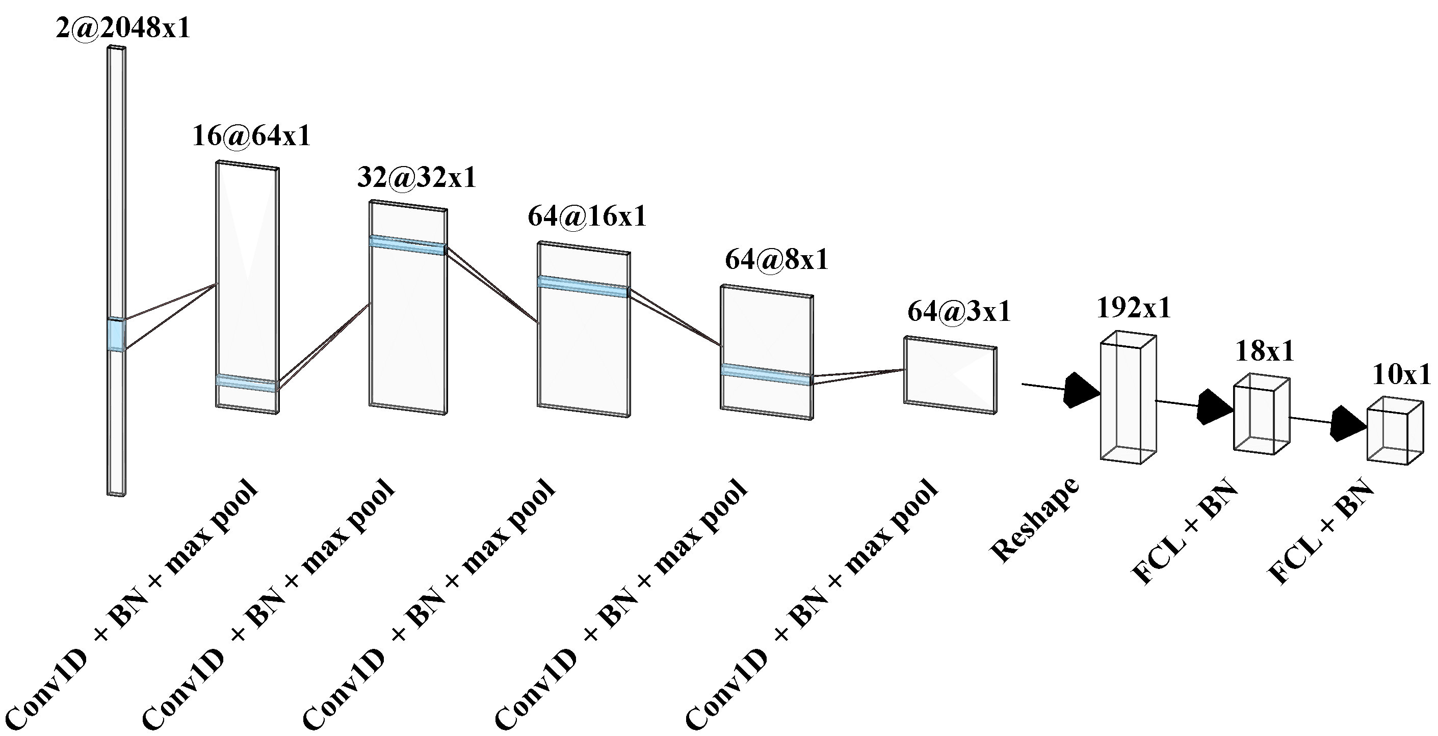
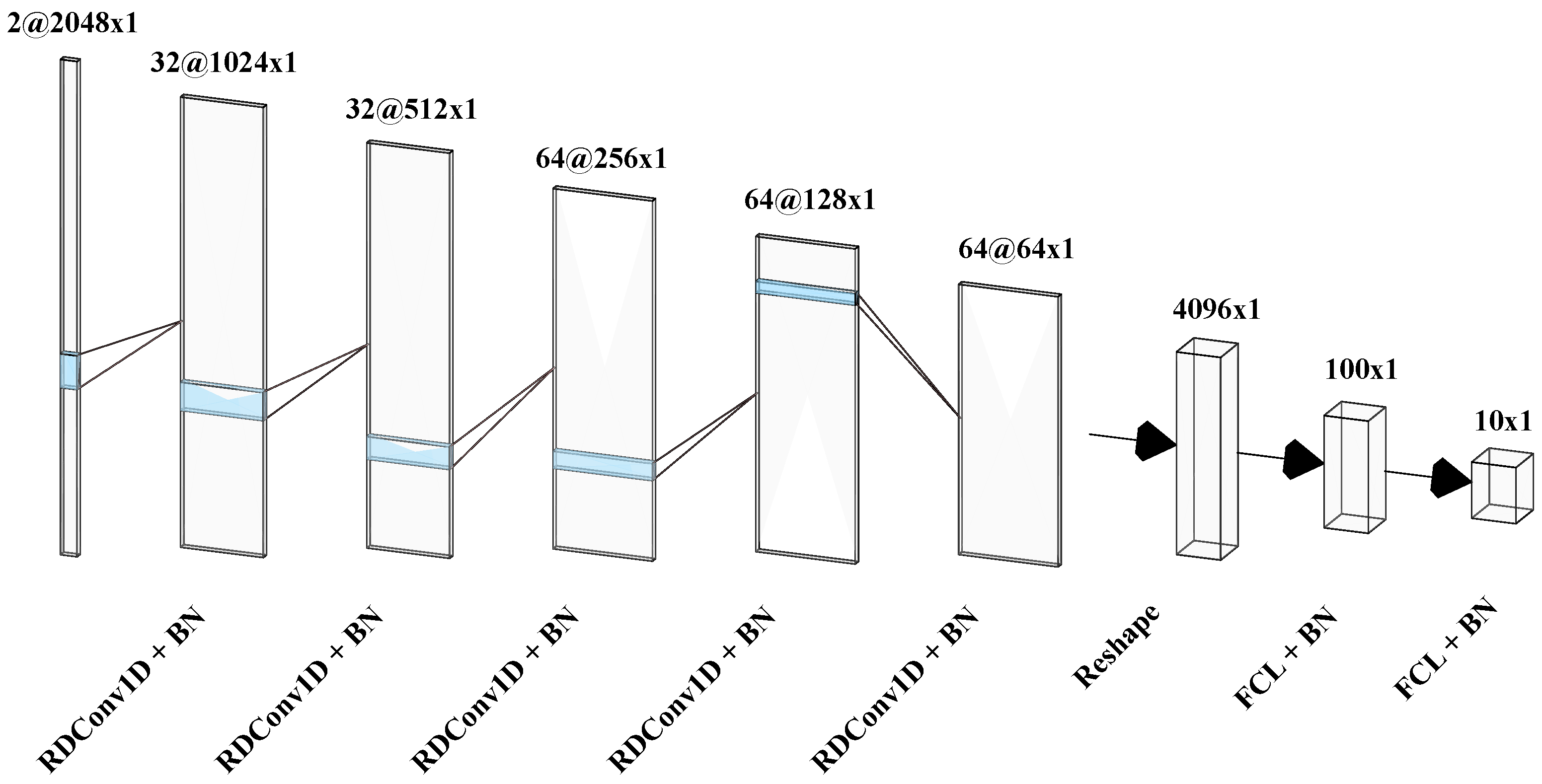
3.1. Model Architectures

Ince’s model [32] was one of the first CNN-based models proposed for vibrationbased fault diagnosis of a rotating system. The original study showed that the model could accurately detect bearing faults from induction motor currents. The original model architecture consists of three CNN layers (Conv1D) and two fully-connected layers (FCL). The original model was slightly modified for the experiments in this study. Table 1 details the modified model architecture. Furthermore, Figure 2 shows the corresponding feature maps between the model layers. The modified version of Ince’s model only employs one fully connected layer. The output space spans over 10 probabilities for every bearing health state in the CWRU dataset. In addition, the output space can include only one value corresponding to the probability of a fault, if the model is optimised for the binary thruster fault detection tasks. Furthermore, BN was placed after every CNN layer, despite BN not being mentioned in the original publication proposing Ince’s model.
WDCNN is an accurate model for vibration based condition monitoring [15]. The model consists of two levels. The first level includes five 1D-CNN, BN and pooling layers employed for feature extraction. The second level includes two fully connected layers with BN for fault recognition. Table 2 details the WDCNN architecture. Furthermore, Figure 3 shows the corresponding feature maps between the model layers. The first layer filters consist of wider 64 × 1 kernels. Each filter includes a kernel for every input channel. The rest of the CNN layers consist of 3 × 1 kernels. After every CNN layer, there is a BN layer, max-pooling layer and a (ReLU) activation function, in this order. All max-pooling layers apply 2 × 1 kernel with a stride of 2. The final fully connected layers compute the probabilities for the system health states.
SRDCNN [18] is a promising model, which achieved relatively high accuracies in bearing fault diagnosis tests in the original study. Similar to Ince’s model and WDCNN, SRDCNN extracts features with 1D convolutional layers and then computes the probabilities for the system health with fully-connected layers. Table 3 lists the main components of SRDCNN architecture. Furthermore, Figure 4 shows the corresponding feature maps between the model layers. The model consists of five convolutional layers and two fully-connected layers. However, the convolutional layers of SRDCNN differ from the convolutional layers of WDCNN and Ince’s model. SRDCNN applies dilated convolutions. Furthermore, each convolutional layer includes two adjacent convolutional sublayers and a residual connection. These adjacent sublayers are structured similarly to the input gates in the recurrent neural network type known as long short-term memory (LSTM). The activation values of these sublayers are multiplied element-wise together and then added element-wise to the residual values. The residual values are the input values to the layer passed through a third adjacent 1D-convolutional sublayer with 1 × 1 kernels. These dilated convolutional layers were named residual dilated convolutional layers (RDConv1D) in the original publication. BN is employed after every convolutional sublayer and fully-connected layer except the convolutional sublayers with 1 × 1 kernels for residual connections.
All these models can function with vibration data from an arbitrary number of sensors. The number of input sensors corresponds to the number of input channels in the first layer of the model. Table 1, Table 2 and Table 3 show that the number of the first layer input channels in all the models in this study is either one or two because the datasets in this study contain vibration data measured with one or two accelerometers. Furthermore, all these models can compute an arbitrary number of probabilities for the health states of the rotor system. The tables in this section show that the output dimensions of the final fully-connected layers of the models can be either 1 or 10. These dimensions correspond to the health states in the two datasets in this study.
Depending on the number of probabilities, this study employs two classification functions computing the diagnosed health state from the probability values. Softmax function, Equation (10), processes the 10 model output values into a probability distribution of 10 probabilities that sum to 1. The diagnosed health state of the system is the label with the highest probability. Sigmoid function, Equation (11), computes the model output value into a probability between [0, 1]. This probability corresponds to the probability of a fault occurring in the system.
S ( z ) = e z j = 0 N e z j
S ( z ) = 1 1 + e z

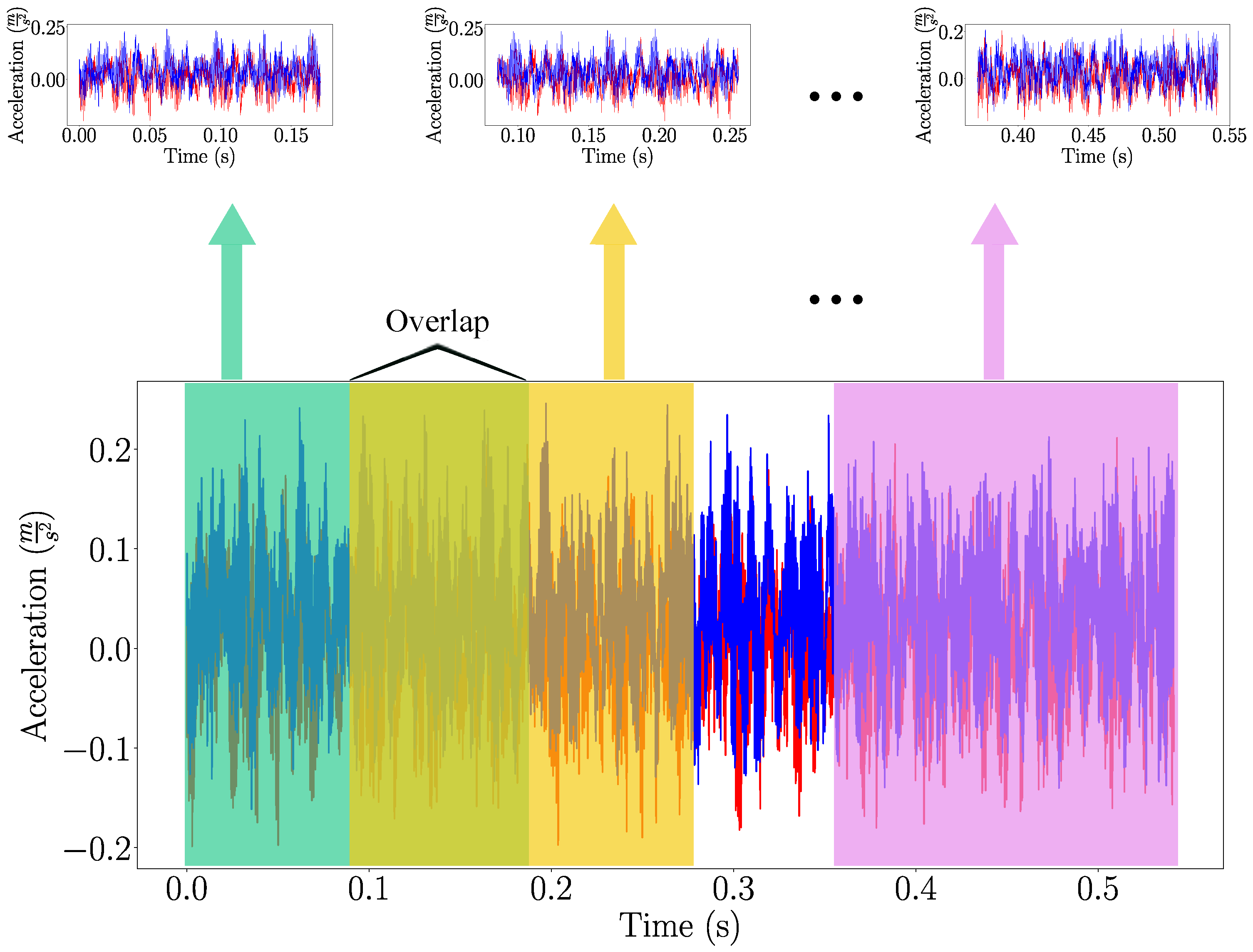
3.2. Whitening CNN Inputs

ND, as proposed in [31], employs the matrix multiplication composition of a convolutional layer, as explained in Section 2.1. ND performs the whitening of the layer input X by subtracting its mean, and then by multiplying it with the inverse square root of the corresponding covariance matrix. Subtracting the mean centres the layer input, and multiplying with the inverse square root of the covariance matrix decorrelates the layer input local area-wise and channel-wise. Ideally, after ND the layer inputs have a mean of zero and the covariance matrix is approximately an identity matrix. The computations related to this whitening operation are shown in the following equations:
Cov = 1 N ( X μ ) T ( X μ )
D ( Cov ) 1 2
y j = ( X μ ) · D · w j + b j .
In Equation (12), the covariance of layer input data is computed. X is the transformed input data matrix and μ are the mean of N values in the columns of X , i.e., the mean of values multiplied by an arbitrary weight. N depends on the number of samples in a minibatch and the number of local areas. D is the deconvolution kernel in Equation (13), which is an approximation of the inverse square root of the covariance matrix. Equation (14) shows the computation of the output values y j of the j-th filter with the centered and transformed input X μ , the deconvolution kernel D COV 1 2 , the filter weights w j and the filter bias terms b j .
The whitening computations, as presented above, may decelerate the optimisation of a deep neural network excessively. Therefore, computation acceleration techniques for ND were also proposed [31]. These techniques include subsampling the layer input matrix X for lighter covariance matrix computation, coupled Newton-Schulz iteration for the inverse square root of the covariance matrix approximation, and implicit decorrelation of layer inputs. This work optimised these acceleration algorithms for the 1D-CNN-based fault diagnosis models. The remainder of this subsection explains the practical implementation of ND and the required acceleration techniques.
After the layer input formulation to matrix X , as shown in Figure 1, the covariance matrix is computed as expressed in Equation (12). Since the covariance matrix computation is performed for every layer and during every forward pass, subsampling the layer input matrices X l likely decreases the required training time. That is, the number of rows N in a layer input matrix X , consisting of local areas from all mini-batch samples, decreases by subsampling the rows. Subsampling is likely to have a small effect on the covariance matrix because the number of input values N is relatively high compared to the covariance matrix dimensions.
To whiten the layer inputs, the inverse square root of the covariance matrix needs to be computed. Several techniques exist for computing the inverse square root of a matrix. However, the coupled Newton-Schulz iteration was shown to be both a numerically stable and fast algorithm for approximating the inverse square root of the covariance matrix [31]. The iteration starts by initialising matrices Y 0 = Cov + ϵ · I and Z 0 = I . The matrices Y k and Z k are updated every iteration with Equations (15) and (16), respectively. The matrices converge to approximate values of the square root and the inverse square root of the covariance matrix, as shown in Formulas (17) and (18).
Y k + 1 = 1 2 Y k ( 3 I Z k Y k )
Z k + 1 = 1 2 ( 3 I Z k Y k ) Z k
Y k + 1 Cov 1 2
Z k + 1 Cov 1 2
Once the inverse square root of the covariance matrix has been approximated, the inverse correction can be applied to the layer input matrix X . However, ND performs this whitening correction implicitly by correcting the weights w of the convolutional layers instead of decorrelating the input data. This whitening can be considered as decorrelating the weights of each kernel in a filter. During training, a running mean of the deconvolution matrix D ( Cov + ϵ · I ) 1 2 is collected for each layer. A small constant ϵ is added for numerical stability and regulatory effect. After training has finished, the running average of the deconvolution kernels D l are frozen and kept constant during testing to reduce the computation time. This implicit deconvolution is expressed mathematically on the right-hand side of Equation (19).
y j l = ( X l μ l ) · ( D l · w j l ) + b j l = X l · D l · w j l + b j l μ l · D l · w j l

3.3. Training the Models

The training convergence of a deep neural network depends heavily on the training algorithm design. With suitable choices, the sample efficiency and the test performance are likely to increase. This work deployed various techniques, such as time window division, learning rate scheduling and early stopping. The following discusses briefly the major choices. The repository for this study is linked in Appendix A for further evaluation.
A disadvantage of deep neural network solutions for fault diagnosis originates from their need for a large number of training samples in order to converge to a satisfying optimum. Fortunately, the number of training samples can be increased with data augmentation. This work employed overlapping time window division for data augmentation. That is, the time series samples were split into shorter time windows including time steps over multiple rotor revolutions. Figure 5 demonstrates this overlapping time window division technique. The extracted time windows correspond to an input sample of 2048 time steps in this study.
The loss function for multi-categorical fault diagnosis tasks is cross-entropy loss (CE loss), as shown in Equation (20). The CE loss is a measure for the difference of the target distribution and the estimated distribution over K categories averaged over N samples in a batch. In Equation (20), y j n { 0 , 1 } are the K values in the target distribution with the correct category encoded as 1 and f j n [ 0 , 1 ] are the K probabilities in the estimated distribution. The loss function for binary fault detection tasks is the binary cross-entropy loss (BCE loss), as shown in Equation (21). Similarly to CE loss, the BCE loss is averaged over the N samples in the batch. In Equation (21), y n { 0 , 1 } is the correct label and f n [ 0 , 1 ] is the probability of a fault.
C E l o s s = 1 N n = 1 N j = 1 K y j n l o g ( f j n )
B C E l o s s = 1 N n = 1 N ( y n l o g ( f n ) + ( 1 y n ) ( 1 l o g ( f n ) )
The gradient optimisation steps of all models were controlled with Adam optimiser [42] and decaying learning rate. The learning rate decayed by half every tenth epoch. Furthermore, all models were optimised with early stopping and checkpoints. That is, at the end of every epoch, if the validation loss decreases, the model weights are saved. If the validation loss increases, the previous best weights are loaded to the model. The optimisation ends after a maximum number of epochs or after the validation loss increases seven times. A maximum number of epochs and other training and model related hyperparameters are detailed in Appendix B.

4. Validation of ND for Fault Diagnosis

This section presents the performance of the baseline models relying on BN and the modified models relying on ND under two different tasks. The first task in Section 4.1 relates to the extensively studied benchmark dataset for bearing fault diagnosis. The dataset consists of rotor system vibration data sampled at different motor loads. The second task in Section 4.2 demonstrates the model’s performance at detecting faults from vibration data acquired in more diverse operating conditions. The dataset of this task consists of thruster vibration data sampled in real operation conditions.

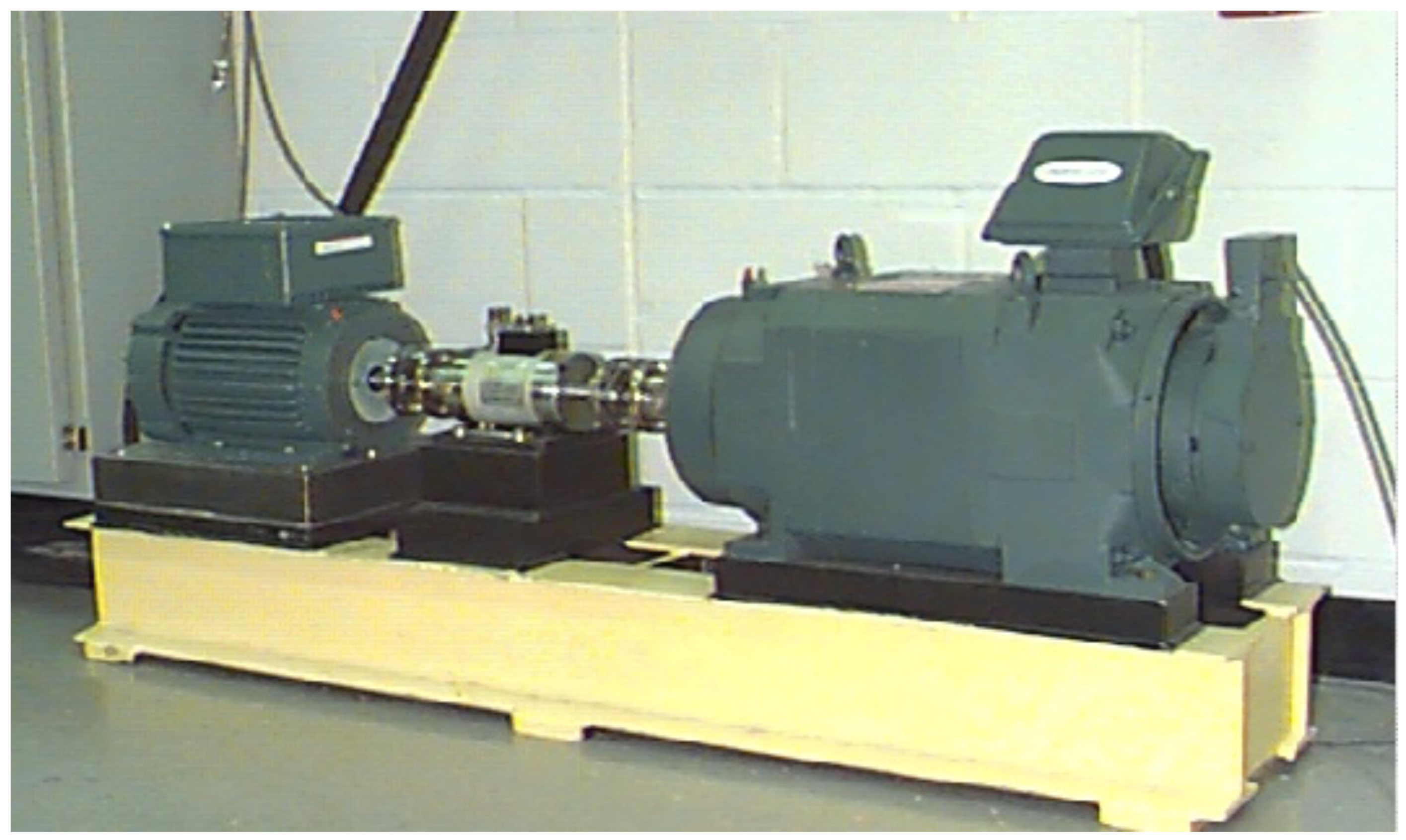
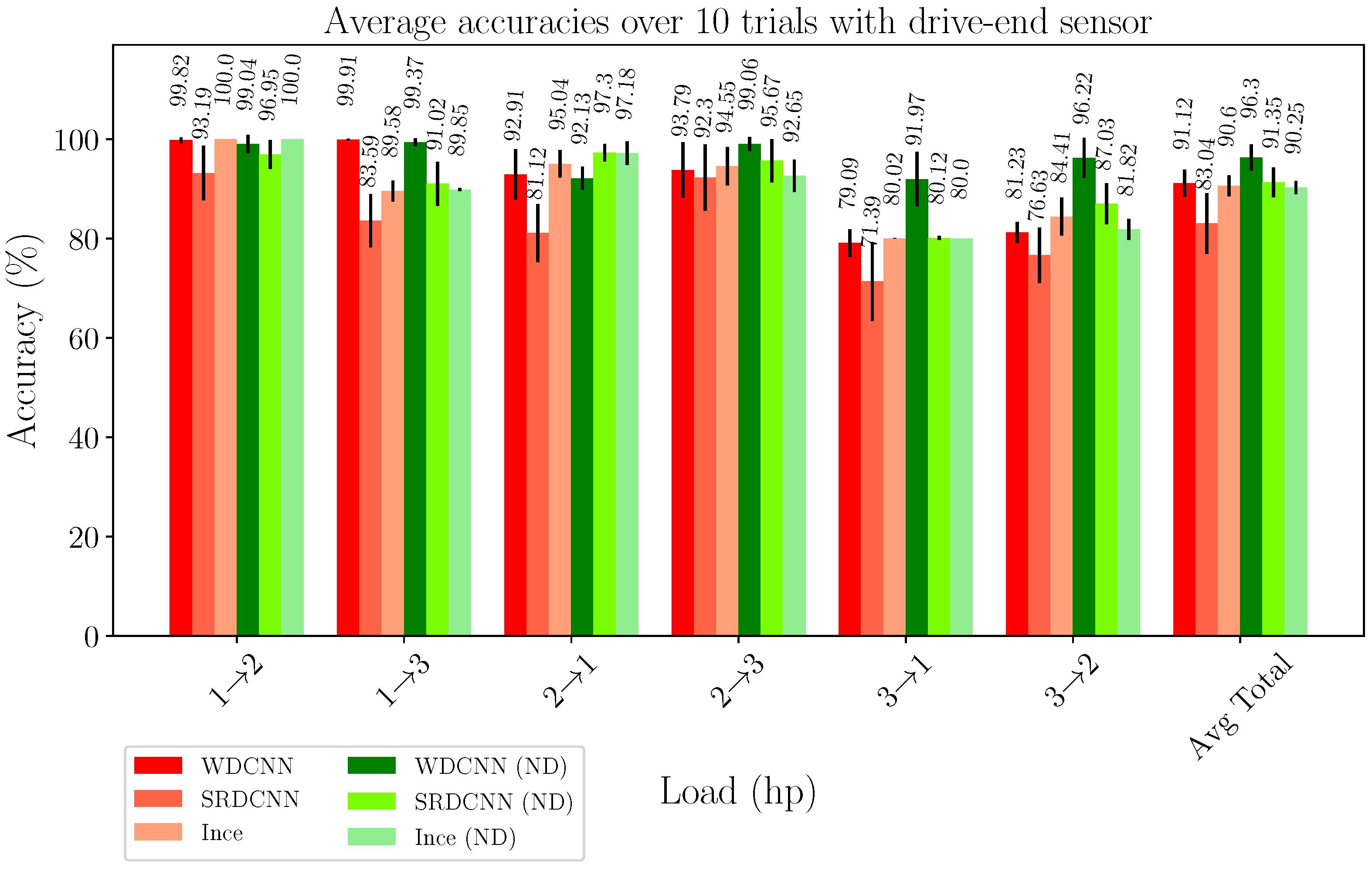
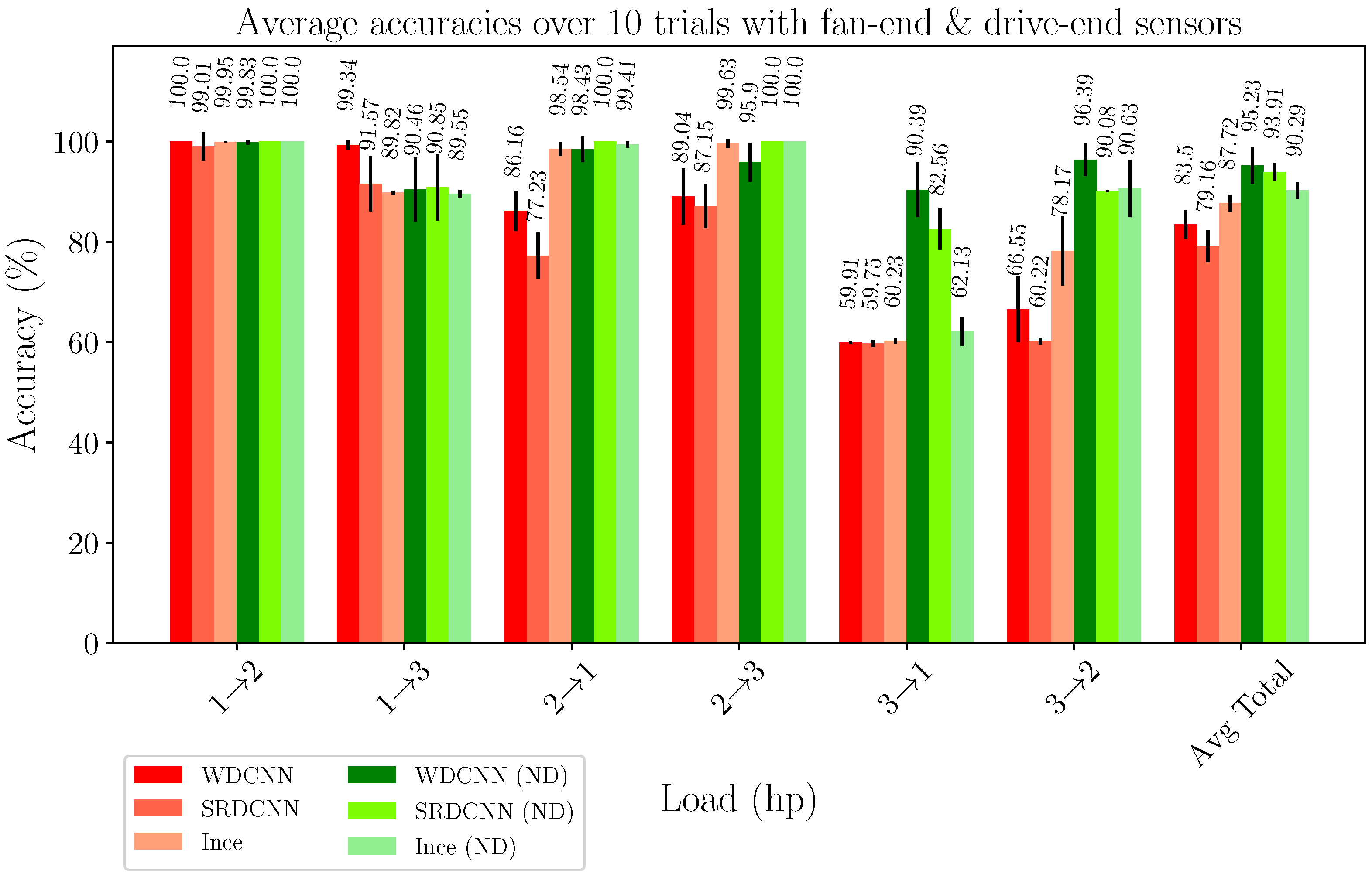
4.1. Case 1: Bearing Fault Diagnosis under Varied Load Conditions

The CWRU bearing fault dataset [33] is a well-established machine fault classification benchmark. The vibration dataset includes samples of healthy and faulty bearings placed in the test rig in Figure 6. There are four different bearing health conditions in the dataset: healthy (H), ball fault (B), inner race fault (I) and outer race fault (O). Each fault type was machined with three different diameters: 0.1778 mm (* L ), 0.3556 mm (* M ) and 0.5334 mm (* H ). Thus, the number of different health states in the dataset is 10. Each fault type was measured at three different motor loads: 0.746 kW (1 hp), 1.491 kW (2 hp) and 2.237 kW (3 hp). Each time series sample was measured with two accelerometers at the drive-end and the fan-end of the motor. The sampling frequency was 12 kHz. Earlier related studies have mostly trained the fault diagnosis models with the vibration data acquired with the drive-end sensor only [15,18,19]. However, often condition monitoring systems include multiple sensors. Therefore, this subsection also presents the fault diagnosis experiments employing both, the drive-end and the fan-end sensor data as model inputs.
Table 4 shows the details related to the bearing fault dataset. The training samples were acquired by sampling overlapping time windows from the 10 time series samples corresponding to the health states. Each training sample is 2048 timesteps long. The shift between adjacent training samples is 32 timesteps. Test samples share the length with training samples, however, they do not overlap.
The baseline models with BN and the modified models with ND were trained to recognise the health state of the bearing from the vibration data. Every model was trained on each motor load domain and then evaluated on the other motor load domains. These tests were repeated 10 times for each model and load domain. Furthermore, these experiments were conducted with data from both accelerometers and with data from the drive-end accelerometer only. Figure 7 presents the means and standard deviations of the model accuracies when only the data from the drive-end accelerometer was available. Figure 8 presents the results from repeated experiments with data from both accelerometers.
Figure 7 shows that all models diagnose the bearing health states with over 80% accuracy on average from the drive-end accelerometer data. In the same experiments, the modified WDCNN and SRDCNN models achieve more than 5 percentage points (pp) better average classification accuracies than the corresponding baseline models. The accuracy of the modified Ince’s model is 0.35 pp less than the corresponding baseline. Overall the modified models achieve similar or significantly better diagnosis accuracies than the corresponding baselines in these experiments.
Figure 8 shows that the average diagnosis accuracies of the models decreased after introducing data from both accelerometers to the task. Only modified Ince’s model and modified SRDCNN increased the diagnostic accuracy compared to the results in Figure 7. Especially the baseline models performed significantly worse when they were trained with data acquired with the motor load of 3 hp. Overall, the average diagnosis accuracies of the modified models were significantly higher than the corresponding baseline counterparts.

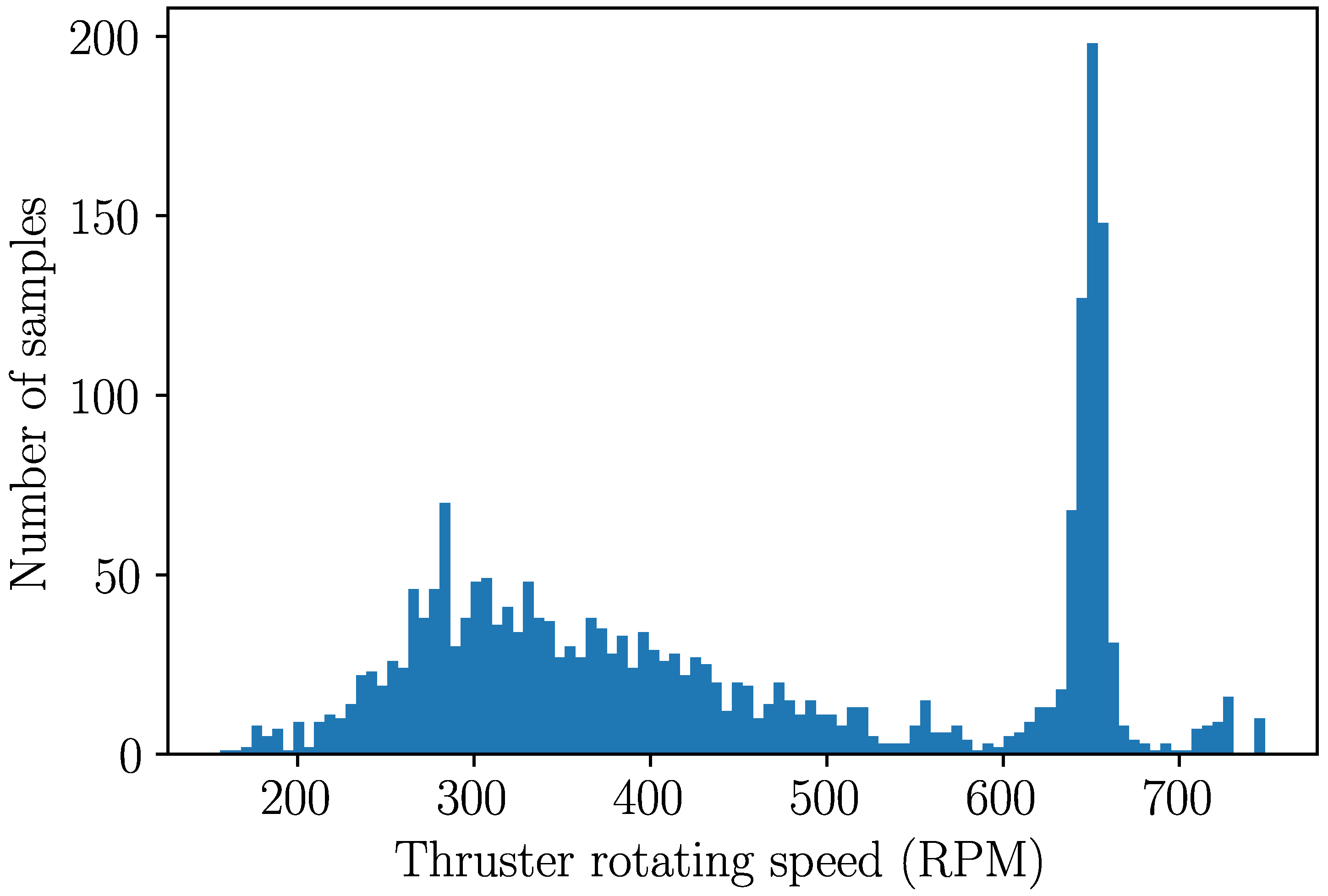
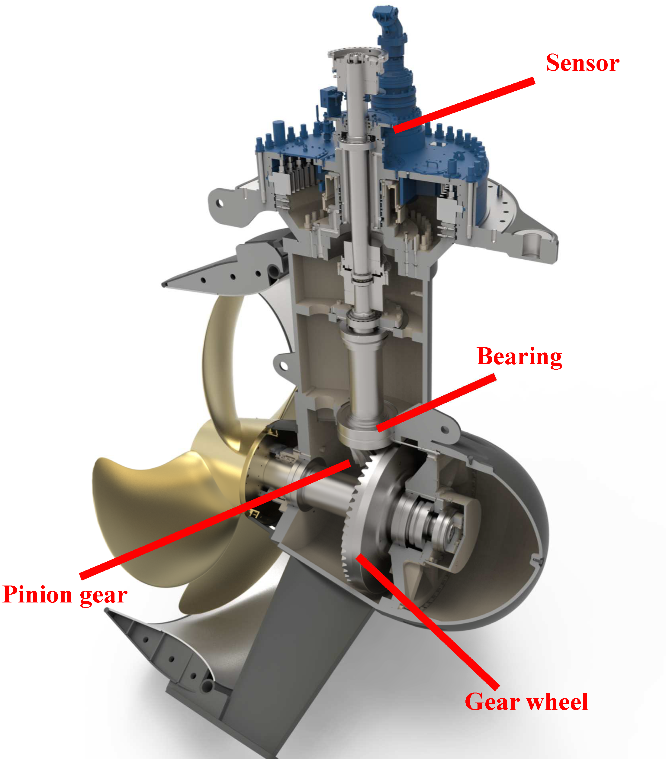
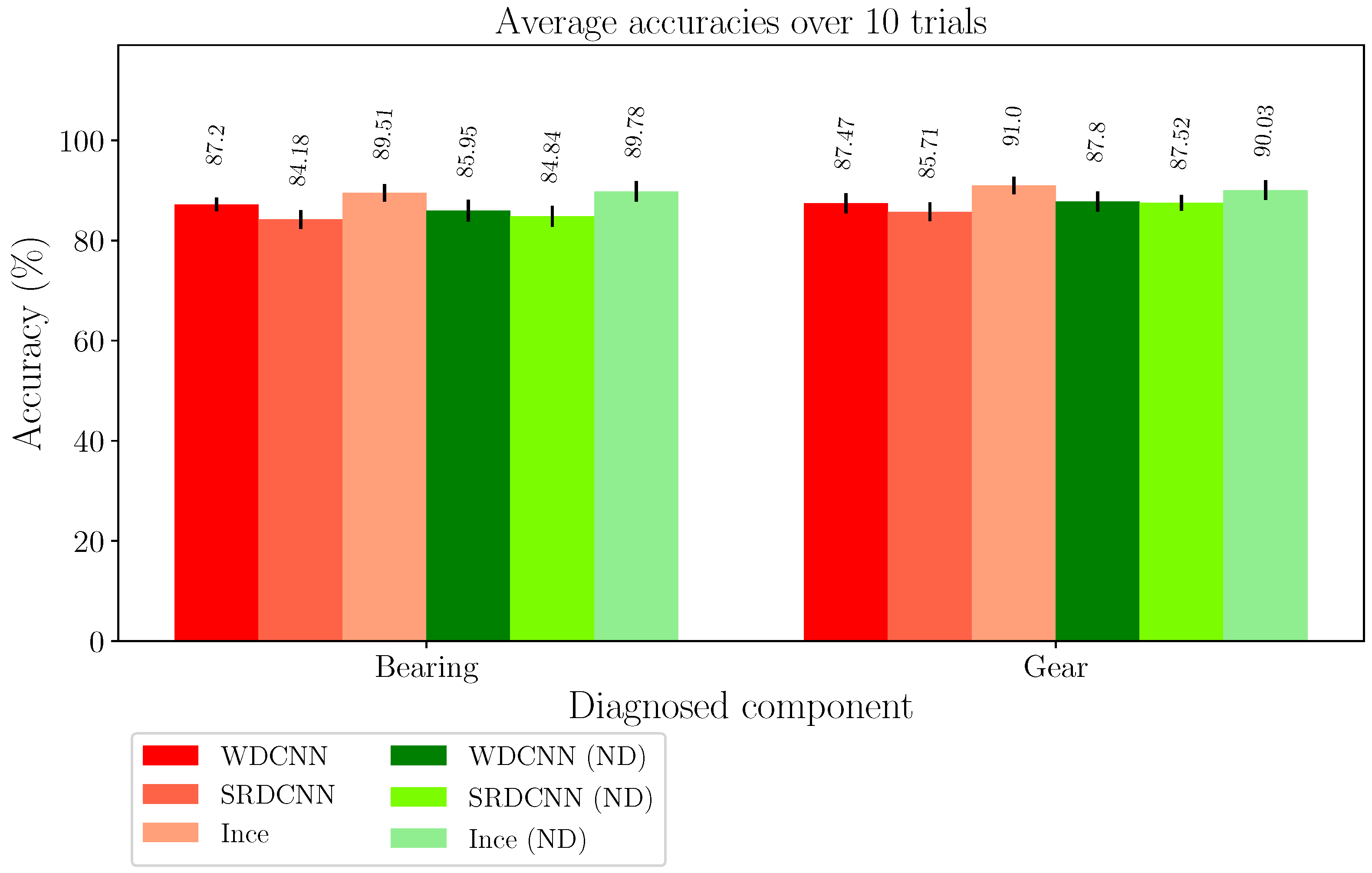
4.2. Case 2: Azimuth Thruster Fault Detection

Three azimuth thrusters of a similar configuration of the same drill ship were monitored frequently from mid-2018 to the end of 2019. An azimuth thruster is a rotor system which ships may use for movement or for preserving position. The three thrusters were operated in diverse environments at various rotating speeds and thrusting angles. Figure 9 shows the rotating speed distribution of the vibration samples in the dataset. Each vibration sample in the dataset is a time series sample including four revolutions sampled at 1024 distinct encoder positions totalling 4096 sampling points. Therefore, the time dimension differs between the vibration samples measured at different rotating speeds.
The vibration samples were acquired with accelerometers in similar positions near the input shafts (IS) of the thrusters. During the monitoring period, the thrusters were healthy in the beginning but suffered malfunctions in matching components. The faults were related to the bearing near the gear end of the pinion shaft (B) and the gear pinion and the gear wheel (G). Figure 10 shows the thruster assembly, the fault locations and the sensor position. All faults occurred in all three thrusters during the period of observations. The faults in the dataset were recognised by condition monitoring specialists.
Some samples with abnormal data were filtered from the dataset with a quality control function. Appendix C describes the quality control function in detail. The resulting dataset is described in Table 5, where the components were either labelled as healthy or faulty. The severity of the faults in a single thruster changes between the samples, due to the long observation period. That is, vibration samples were collected over a long period of time before and after the malfunctions were first noticed.
The lowest row in Table 5 shows the number of samples drawn and augmented to training, validation and test datasets. The relatively high number of training, validation and test samples is due to data augmentation with time window division. Each time window was 2048 time steps long. The time windows were overlapped during training data and validation data augmentation, but not overlapped during test data augmentation. The same number of samples were drawn randomly 10 times for each trial consisting of training and evaluation of all models. Furthermore, each set holds an equal number of healthy and faulty samples.
The baseline models with BN and the modified models with ND were optimised to recognise faulty behaviour in a specific component. Therefore, the models were subjected to binary classification tasks. All models were trained and then evaluated 10 times for each task with the hyperparameters listed in Appendix B. Figure 11 shows the average test classification accuracies of the models in the fault diagnosis tasks. All models achieved similar diagnosis accuracies between 84% and 91% in both tasks. Overall, the modified models with ND performed slightly better. The modified SRDCNN and Ince’s model diagnosed the bearing condition less than 1 pp more accurately than the corresponding baseline models. Moreover, the modified WDCNN and SRDCNN diagnosed the bearing condition less than 2 pp more accurately than the corresponding baseline models.

5. Discussion

Based on the results, ND seems like a competitive solution for BN in CNN-based machine fault diagnosis from vibration data. In Section 4.1, the modified models with ND were compared to the baseline models with a well-established benchmark dataset for bearing fault diagnosis. In this multi-categorical bearing fault recognition task, the modified models with ND mostly outperformed the baseline models with BN in terms of the average accuracy of all experiments. Whitening seemed to especially improve WDCNN performance. The average accuracy of modified WDCNN was 5.18 pp and 11.73 pp higher than the baseline in results shown in Figure 7 and Figure 8, respectively. Furthermore, the modified WDCNN and modified SRDCNN outperformed remarkably the corresponding baselines in experiments with training data drawn from the vibration data sampled at a 3 hp motor load.
In Section 4.2, the modified models and the baseline models were compared by using a real world dataset consisting of ship thrusters in diverse environments. In these thruster fault detection tasks, all models achieved relatively high accuracies of over 84%. However, there were no significant differences between the fault detection accuracies of the compared models. Based on these thruster fault detection tasks, ND can be considered as good as BN for normalising the activations of CNN-based fault detection models.
Although ND is a promising technique for whitening the features between CNN layers, it introduces a few extra hyperparameters for fault diagnosis model training. Moreover, the models relying on ND can be very sensitive toward these hyperparameters. That is, the sampling stride, the number of coupled Newton-Schulz iterations and the regularisation term ϵ , for example, may affect optimisation results and require careful tuning. For convenience, Appendix D shows accuracies at different subsampling strides and batch sizes. Furthermore, Appendix E provides some examples of the deconvolution matrix D after a different number of coupled Newton-Schulz iterations. Fortunately, similar ND hyperparameters seemed to perform well in both model validation case studies, even though the data was significantly different due to the measurement circumstances and due to the health state spaces. Therefore, the values searched in this work for ND hyperparameters are likely suitable for other vibration diagnosis tasks.
Overall, whitening the layer inputs seems to consistently provide high test performance for CNN-based fault diagnosis models. By whitening the layer inputs, the model learns uncorrelated features containing less redundant information than correlated features. With uncorrelated features, the domain adaptation of the model improves on average, as shown in Section 4.1. The difference in domain adaptation between whitened features and batch normalised features is significant, especially when shifting from the higher load domains to lower load domains. Furthermore, decor-related features seem to significantly increase the accuracies of the diagnosis models compared to the baseline models when data from two sensors were employed, as Figure 8 shows. This indicates that decorrelating CNN-based model features may increase fault diagnosis accuracy of condition monitoring systems with many sensors.

6. Conclusions

This study demonstrated the effect of whitening the features of 1D-CNN-based fault diagnosis models. The features of three commonly known and highly accurate fault diagnosis models were whitened with network deconvolution. Network deconvolution is a recently proposed, implicit and approximative whitening technique. The models modified with network deconvolution were compared to the originally proposed models relying on batch normalisation under two validation case studies. In the first case study, the models were evaluated on a well established bearing fault dataset under varied load domains. The second case study evaluated the model performances in more challenging real thruster fault detection tasks. The first case study showed that whitened features increased the 1D-CNN model performances on average. Furthermore, the same case study showed that the models with whitened features were significantly more accurate at diagnosing the bearing health state from the vibration data acquired with two sensors. However, the second case study showed that the models with whitened features achieved similar fault detection accuracies to the corresponding baseline models. Overall, this study shows that whitening 1D-CNN-based fault diagnosis model features may improve the diagnosis performance. These results are significant for CNN-based fault diagnosis algorithms since the whitening technique employed in this study can replace all batch normalisation layers in any CNN-based fault diagnosis model.

Author Contributions

Conceptualization, J.M., R.-P.N. and J.K.-R.; methodology, J.M.; software, J.M.; validation, J.M., R.-P.N., J.K.-R., F.F. and T.T.; formal analysis, J.M.; investigation, J.M.; resources, J.M.; data curation, J.M., R.-P.N. and J.K.-R.; writing—original draft preparation, J.M.; writing—review and editing, J.M., R.-P.N., J.K.-R., F.F., T.T., S.S. and R.V.; visualization, J.M.; supervision, J.K.-R., F.F., T.T., S.S. and R.V; project administration, J.K.-R. and R.V.; funding acquisition, J.K.-R. and R.V. All authors have read and agreed to the published version of the manuscript.

Funding

This research was funded by Business Finland as part of the Reboot IoT project (grant number 4356/31/2019) and by the Academy of Finland as part of the AI-ROT research project (grant number 335717).

Institutional Review Board Statement

Not applicable.

Data Availability Statement

Data sharing concerning the thruster dataset is not applicable to this article due to legal issues. Publicly available datasets were analyzed in this study. This data, concerning the bearing fault dataset, can be found here: https://engineering.case.edu/bearingdatacenter.

Conflicts of Interest

The authors declare no conflict of interest. The funders had no role in the design of the study; in the collection, analyses, or interpretation of data; in the writing of the manuscript, or in the decision to publish the results.

Abbreviations

The following abbreviations are used in this manuscript:
IFDIntelligent Fault Diagnosis
BNBatch Normalization
NDNetwork Deconvolution
CNNConvolutional Neural Network
DLDeep Learning
MLMachine Learning
DBNDeep Belief Network
AEAutoencoder
RNNRecurrent Neural Network
WDCNNDeep Convolutional Neural Networks with Wide First-layer Kernels
SRDCNNStacked Residual Dilated Convolutional Neural Network
ReLURectified Linear Unit
LSTMLong Short-Term Memory
CECross-Entropy
BCEBinary Cross-Entropy
ppPercentage Point

Appendix A. Source Code

The repository linked below contains the source code related to this study.

Appendix B. Model Specific Hyperparameters

Before the model optimisation, some of the training related and model related hyperparameters were optimised for every model separately. Table A1 lists the hyperparameters employed in the bearing fault diagnosis experiments in Section 4.1. Table A2 details the hyperparameters of the thruster experiments in Section 4.2. The models marked with ‘ND’ in parenthesis refer to the models modified with network deconvolution. First layer iterations refers to the number of coupled Newton-Schulz iterations at the first convolutional layer. Deconv iterations refers to the number of coupled Newton-Schulz iterations on other model layers. ϵ is the small constant for regularisation and numerical stability of the iteration. Sampling stride defines the subsampling factor for the layer input matrix X .
Table A1. Hyperparameters deployed in bearing fault experiments *.
ParamInceSRDCNNWDCNNInce (ND)SRDCNN (ND)WDCNN (ND)
Batch size3264648128 (8)8
Learning rate0.0010.00010.0010.00010.1 (0.0001)0.0001
Max epochs606070704070
BiasFalseTrueTrueTrueTrueTrue
First layer iterationsN/AN/AN/A151515
Deconv iterationsN/AN/AN/A555
ϵ N/AN/AN/A 10 5 10 5 10 5
Sampling strideN/AN/AN/A555
* Hyperparameters employed in experiments with the drive-end and the fan-end sensors are in parentheses if different.
Table A2. Hyperparameters deployed in thruster fault experiments.
ParamInceSRDCNNWDCNNInce (ND)SRDCNN (ND)WDCNN (ND)
Batch size326464888
Learning rate0.0010.00010.0010.00010.00010.0001
Max epochs606070707070
BiasFalseTrueTrueTrueTrueTrue
First layer iterationsN/AN/AN/A151525
Deconv iterationsN/AN/AN/A555
ϵ N/AN/AN/A 10 5 10 5 10 5
Sampling strideN/AN/AN/A5536

Appendix C. Quality Control Function for Filtering Abnormal Samples

Although the thruster data was sampled in diverse environments and the time series samples differed, some samples containing outliers were removed from the dataset. Outlier samples originated likely due to many reasons, such as faulty sensor or heavy storm conditions. For this purpose, a quality control algorithm was developed to reject the outlying samples based on three checks. Firstly, the data sample consisting of 4096 × 1 time series was divided into sliding time windows of 100 × 1, with the step size of 1. A mean value was then computed for all the sliding windows. The sample was rejected if the difference between the maximum and the minimum mean value was higher than 0.2 × 9.81 m/s 2 . Secondly, the sample was rejected if the maximum and minimum values of the time series were the same. Thirdly, the sample was rejected if the absolute mean of the time series was over 0.5 × 9.81 m/s 2 . If the sample passed each check, it was accepted for further processing.

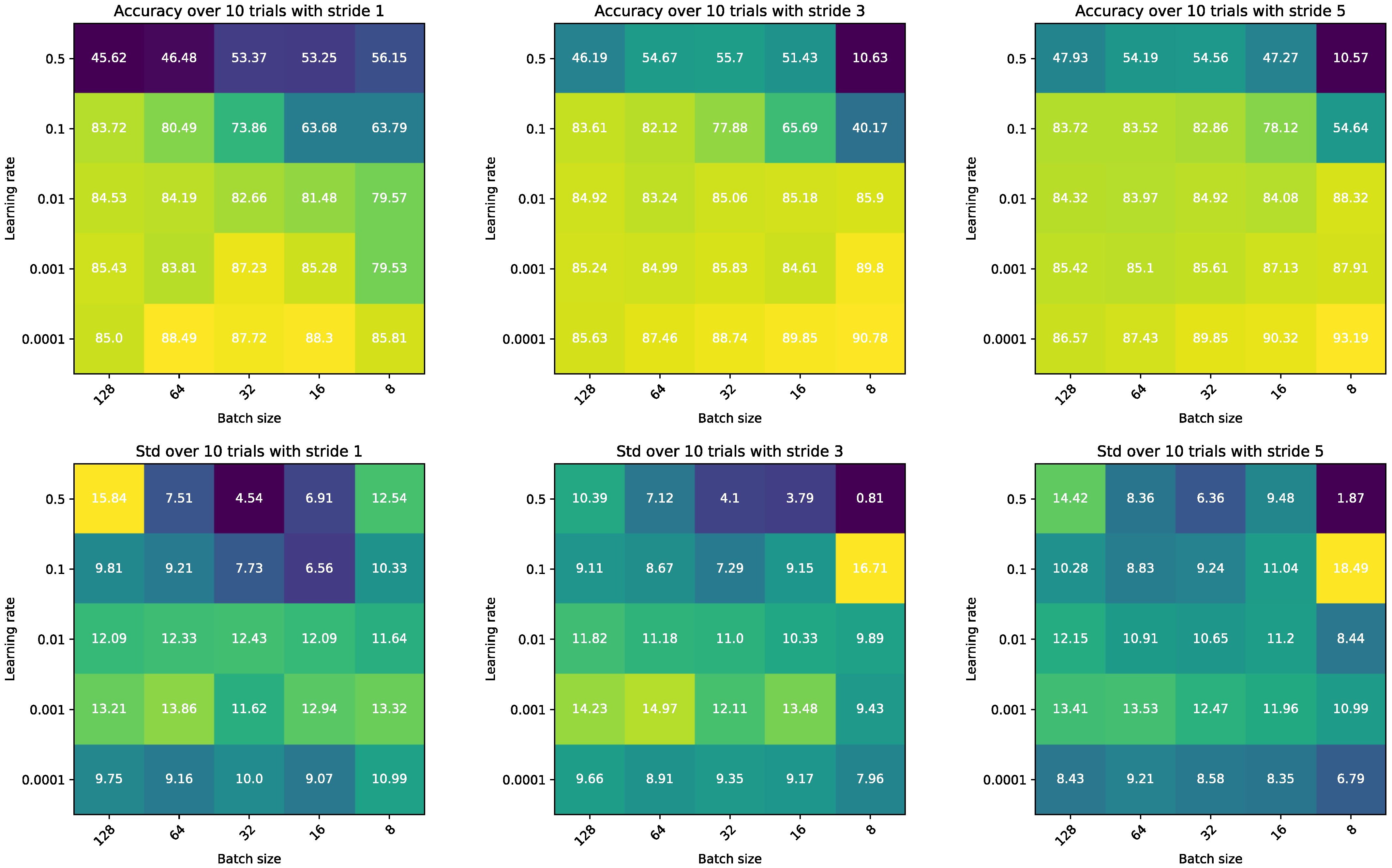
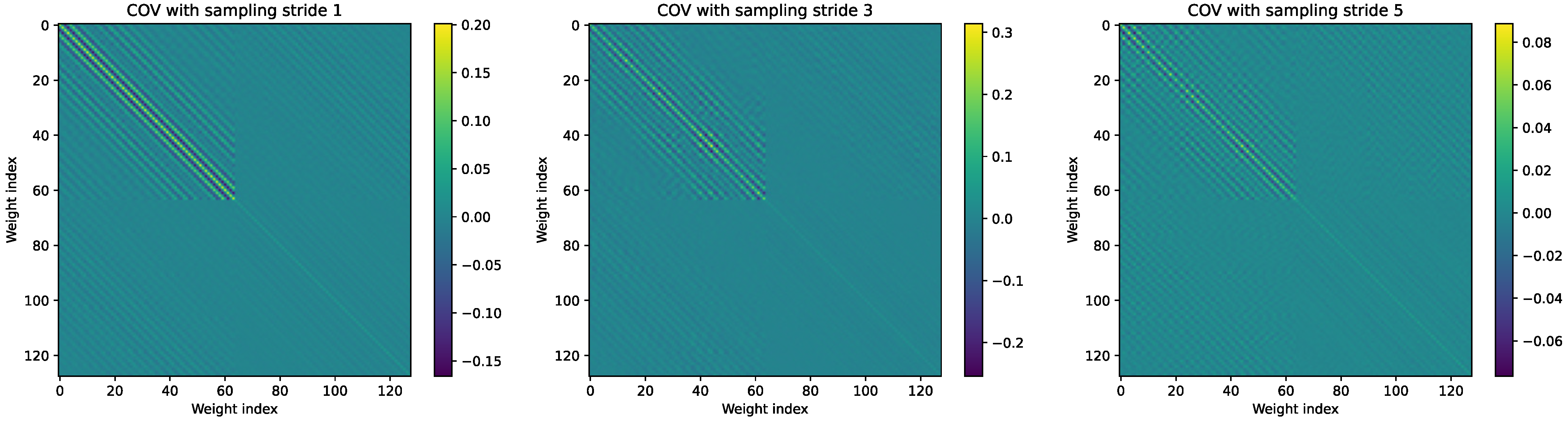
Appendix D. Batch Size and Sampling Stride Effect on ND

The batch size and sampling stride both affect the number of values in the layer input X , as in Figure 1. With larger batch sizes, the number of values in each column increases. With higher sampling strides, the number of values in each column decreases. The number of values in each column correlates with the representability of the covariance matrix, and thus affects the decorrelation reliability. With a low number of inputs per neuron, the covariance matrix might not represent the true input distribution over the whole dataset. Therefore, the sampling stride and batch size were searched. Figure A1 shows three different grid search results for batch size, sampling stride and learning rate. The model in this grid search was WDCNN and the input data included vibration data from the fan-end and the drive-end sensors. Each accuracy in the figure corresponds to average accuracy of six load domain shift tasks, as in Section 4.1. The experiments were repeated 10 times with less than 20 training epochs. Each standard deviation in the figure corresponds to the distribution of all load domain shift test accuracies over the ten experiments. In addition, Figure A2 visualises covariance matrices of the WDCNN first layer inputs corresponding to a random sample with drive-end and fan-end data from the bearing fault dataset. The covariance matrices are computed with different sampling strides. Figure A2 shows that the covariance between the inputs decreases as the sampling stride increases.
Figure A1. Mean and standard deviations of WDCNN test accuracies over 10 trials of load domain shift tests with the bearing fault dataset. Specifically, each accuracy and standard deviation in the figure is the total average of the six load domain shift results, similar to the ones in Section 4.1.
Applsci 12 04411 g0a1
Figure A2. Covariance matrices of the first layer input related to a batch of vibration samples with two channels (fan-end and drive-end sensors) from the bearing fault dataset. The sampling stride corresponds to the sampling strides in Figure A1. The covariance is highest between inputs in the same channel (diagonal corner quarters of the heatmaps) and between the nearby weights within a kernel. The first layer filter of WDCNN has two kernels of size 64 × 1, which explains the covariance matrix dimension of 128 × 128.
Applsci 12 04411 g0a2

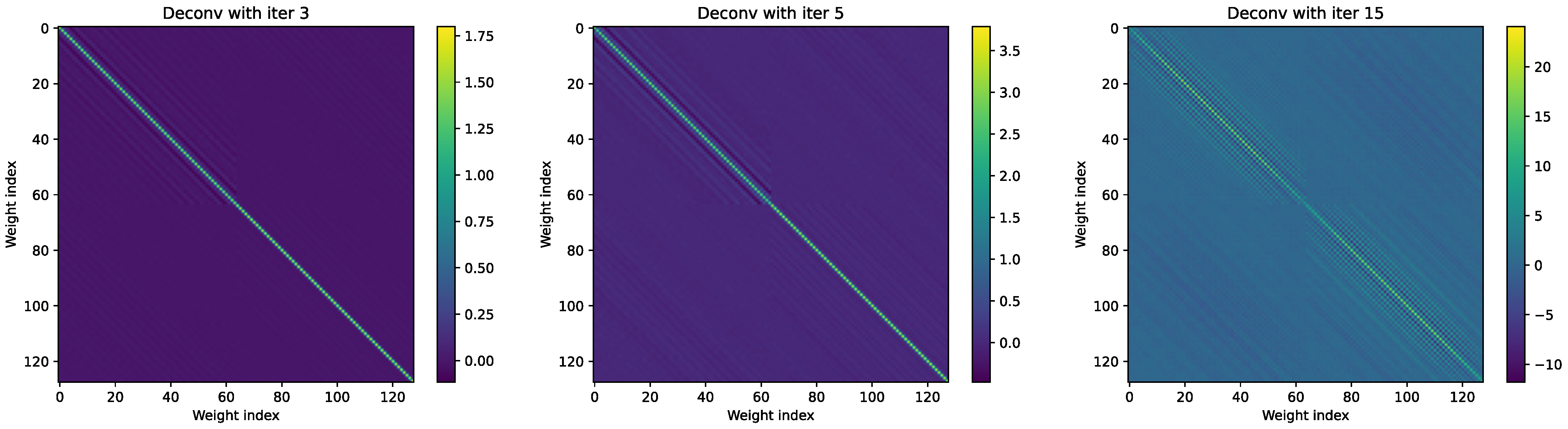
Appendix E. Iteration Count Effect on the Approximation of the Deconvolution Kernel

The coupled Newton-Schulz iteration for approximating the inverse square root of the covariance of layer input matrix X converges to values with more contrast as the number of iterations increases. Figure A3 shows these deconvolution matrices approximated with different number of iterations.
Figure A3. Three deconvolution matrices with different number of iterations approximated from the leftmost covariance matrix in Figure A2. The deconvolution matrix approximation grow significantly sharper as the number of iterations increase.
Applsci 12 04411 g0a3

References

  1. Lei, Y.; Yang, B.; Jiang, X.; Jia, F.; Li, N.; Nandi, A.K. Applications of machine learning to machine fault diagnosis: A review and roadmap. Mech. Syst. Signal Process. 2020, 138, 106587. [Google Scholar] [CrossRef]
  2. Liu, R.; Yang, B.; Zio, E.; Chen, X. Artificial intelligence for fault diagnosis of rotating machinery: A review. Mech. Syst. Signal Process. 2018, 108, 33–47. [Google Scholar] [CrossRef]
  3. Lei, Y.; Zuo, M.J.; He, Z.; Zi, Y. A multidimensional hybrid intelligent method for gear fault diagnosis. Expert Syst. Appl. 2010, 37, 1419–1430. [Google Scholar] [CrossRef]
  4. Yang, B.S.; Di, X.; Han, T. Random forests classifier for machine fault diagnosis. J. Mech. Sci. Technol. 2008, 22, 1716–1725. [Google Scholar] [CrossRef]
  5. Widodo, A.; Yang, B.S. Support vector machine in machine condition monitoring and fault diagnosis. Mech. Syst. Signal Process. 2007, 21, 2560–2574. [Google Scholar] [CrossRef]
  6. Witczak, M.; Korbicz, J.; Mrugalski, M.; Patton, R.J. A GMDH neural network-based approach to robust fault diagnosis: Application to the DAMADICS benchmark problem. Control Eng. Pract. 2006, 14, 671–683. [Google Scholar] [CrossRef]
  7. Hinton, G.E. Learning multiple layers of representation. Trends Cogn. Sci. 2007, 11, 428–434. [Google Scholar] [CrossRef] [PubMed]
  8. Li, C.; Sanchez, R.V.; Zurita, G.; Cerrada, M.; Cabrera, D.; Vásquez, R.E. Multimodal deep support vector classification with homologous features and its application to gearbox fault diagnosis. Neurocomputing 2015, 168, 119–127. [Google Scholar] [CrossRef]
  9. Lu, C.; Wang, Z.Y.; Qin, W.L.; Ma, J. Fault diagnosis of rotary machinery components using a stacked denoising autoencoder-based health state identification. Signal Process. 2017, 130, 377–388. [Google Scholar] [CrossRef]
  10. Zhao, R.; Yan, R.; Chen, Z.; Mao, K.; Wang, P.; Gao, R.X. Deep learning and its applications to machine health monitoring. Mech. Syst. Signal Process. 2019, 115, 213–237. [Google Scholar] [CrossRef]
  11. Khan, S.; Yairi, T. A review on the application of deep learning in system health management. Mech. Syst. Signal Process. 2018, 107, 241–265. [Google Scholar] [CrossRef]
  12. Shao, H.; Jiang, H.; Zhang, H.; Duan, W.; Liang, T.; Wu, S. Rolling bearing fault feature learning using improved convolutional deep belief network with compressed sensing. Mech. Syst. Signal Process. 2018, 100, 743–765. [Google Scholar] [CrossRef]
  13. Malhotra, P.; Ramakrishnan, A.; Anand, G.; Vig, L.; Agarwal, P.; Shroff, G. LSTM-based Encoder-Decoder for Multi-sensor Anomaly Detection. arXiv 2016, arXiv:1607.00148. [Google Scholar]
  14. Zhang, S.; Zhang, S.; Wang, B.; Habetler, T.G. Deep Learning Algorithms for Bearing Fault Diagnostics—A Comprehensive Review. IEEE Access 2020, 8, 29857–29881. [Google Scholar] [CrossRef]
  15. Zhang, W.; Peng, G.; Li, C.; Chen, Y.; Zhang, Z. A New Deep Learning Model for Fault Diagnosis with Good Anti-Noise and Domain Adaptation Ability on Raw Vibration Signals. Sensors 2017, 17, 425. [Google Scholar] [CrossRef]
  16. Zhang, W.; Li, C.; Peng, G.; Chen, Y.; Zhang, Z. A deep convolutional neural network with new training methods for bearing fault diagnosis under noisy environment and different working load. Mech. Syst. Signal Process. 2018, 100, 439–453. [Google Scholar] [CrossRef]
  17. Shenfield, A.; Howarth, M. A Novel Deep Learning Model for the Detection and Identification of Rolling Element-Bearing Faults. Sensors 2020, 20, 5112. [Google Scholar] [CrossRef]
  18. Zhuang, Z.; Lv, H.; Xu, J.; Huang, Z.; Qin, W. A Deep Learning Method for Bearing Fault Diagnosis through Stacked Residual Dilated Convolutions. Appl. Sci. 2019, 9, 1823. [Google Scholar] [CrossRef] [Green Version]
  19. Hendriks, J.; Dumond, P.; Knox, D. Towards better benchmarking using the CWRU bearing fault dataset. Mech. Syst. Signal Process. 2022, 169, 108732. [Google Scholar] [CrossRef]
  20. Janssens, O.; Slavkovikj, V.; Vervisch, B.; Stockman, K.; Loccufier, M.; Verstockt, S.; Van de Walle, R.; Van Hoecke, S. Convolutional Neural Network Based Fault Detection for Rotating Machinery. J. Sound Vib. 2016, 377, 331–345. [Google Scholar] [CrossRef]
  21. Jing, L.; Zhao, M.; Li, P.; Xu, X. A convolutional neural network based feature learning and fault diagnosis method for the condition monitoring of gearbox. Measurement 2017, 111, 1–10. [Google Scholar] [CrossRef]
  22. Zhao, D.; Wang, T.; Chu, F. Deep convolutional neural network based planet bearing fault classification. Comput. Ind. 2019, 107, 59–66. [Google Scholar] [CrossRef]
  23. Han, T.; Liu, C.; Yang, W.; Jiang, D. A novel adversarial learning framework in deep convolutional neural network for intelligent diagnosis of mechanical faults. Knowl.-Based Syst. 2019, 165, 474–487. [Google Scholar] [CrossRef]
  24. Guo, L.; Lei, Y.; Xing, S.; Yan, T.; Li, N. Deep Convolutional Transfer Learning Network: A New Method for Intelligent Fault Diagnosis of Machines With Unlabeled Data. IEEE Trans. Ind. Electron. 2019, 66, 7316–7325. [Google Scholar] [CrossRef]
  25. Yang, B.; Lei, Y.; Jia, F.; Xing, S. An intelligent fault diagnosis approach based on transfer learning from laboratory bearings to locomotive bearings. Mech. Syst. Signal Process. 2019, 122, 692–706. [Google Scholar] [CrossRef]
  26. Ioffe, S.; Szegedy, C. Batch Normalization: Accelerating Deep Network Training by Reducing Internal Covariate Shift. arXiv 2015, arXiv:cs.LG/1502.03167. [Google Scholar]
  27. Huang, L.; Qin, J.; Zhou, Y.; Zhu, F.; Liu, L.; Shao, L. Normalization techniques in training DNNs: Methodology, analysis and application. arXiv 2020, arXiv:2009.12836. [Google Scholar]
  28. LeCun, Y.A.; Bottou, L.; Orr, G.B.; Müller, K.R. Efficient backprop. In Neural networks: Tricks of the Trade; Springer: Berlin/Heidelberg, Germany, 2012; pp. 9–48. [Google Scholar] [CrossRef]
  29. Huang, L.; Zhou, L.Z.Y.; Zhu, F.; Liu, L.; Shao, L. An investigation into the stochasticity of batch whitening. In Proceedings of the IEEE Computer Society Conference on Computer Vision and Pattern Recognition, Seattle, WA, USA, 14–19 June 2020; pp. 6438–6447. [Google Scholar] [CrossRef]
  30. Huang, L.; Yang, D.; Lang, B.; Deng, J. Decorrelated Batch Normalization. In Proceedings of the IEEE Conference on Computer Vision and Pattern Recognition (CVPR), Salt Lake City, UT, USA, 18–23 June 2018. [Google Scholar]
  31. Ye, C.; Evanusa, M.; He, H.; Mitrokhin, A.; Goldstein, T.; Yorke, J.A.; Fermuller, C.; Aloimonos, Y. Network Deconvolution. In Proceedings of the International Conference on Learning Representations, Addis Ababa, Ethiopia, 26–30 April 2020. [Google Scholar]
  32. Ince, T.; Kiranyaz, S.; Eren, L.; Askar, M.; Gabbouj, M. Real-Time Motor Fault Detection by 1-D Convolutional Neural Networks. IEEE Trans. Ind. Electron. 2016, 63, 7067–7075. [Google Scholar] [CrossRef]
  33. Case Western Reserve University Bearing Data Center. Case Western Reserve University Bearing Data Center Website. Available online: https://engineering.case.edu/bearingdatacenter (accessed on 5 April 2022).
  34. Scherer, D.; Müller, A.; Behnke, S. Evaluation of pooling operations in convolutional architectures for object recognition. In Proceedings of the International Conference on Artificial Neural Networks, Thessaloniki, Greece, 15–18 September 2010; pp. 92–101. [Google Scholar]
  35. He, K.; Zhang, X.; Ren, S.; Sun, J. Deep Residual Learning for Image Recognition. In Proceedings of the 2016 IEEE Conference on Computer Vision and Pattern Recognition (CVPR), Las Vegas, NV, USA, 27–30 June 2016; pp. 770–778. [Google Scholar] [CrossRef] [Green Version]
  36. Huang, G.; Liu, Z.; van der Maaten, L.; Weinberger, K.Q. Densely Connected Convolutional Networks. In Proceedings of the IEEE Conference on Computer Vision and Pattern Recognition (CVPR), Las Vegas, NV, USA, 27–30 June 2016. [Google Scholar]
  37. Xie, S.; Girshick, R.; Dollar, P.; Tu, Z.; He, K. Aggregated Residual Transformations for Deep Neural Networks. In Proceedings of the IEEE Conference on Computer Vision and Pattern Recognition (CVPR), Las Vegas, NV, USA, 27–30 June 2016. [Google Scholar]
  38. He, K.; Gkioxari, G.; Dollar, P.; Girshick, R. Mask R-CNN. In Proceedings of the IEEE International Conference on Computer Vision (ICCV), Venice, Italy, 22–29 October 2017. [Google Scholar]
  39. Desjardins, G.; Simonyan, K.; Pascanu, R.; Kavukcuoglu, K. Natural Neural Networks. In Proceedings of the NIPS’15: 28th International Conference on Neural Information Processing Systems, Montreal, QC, Canada, 7–12 December 2015; Volume 2, pp. 2071–2079. [Google Scholar]
  40. Luo, P. Learning Deep Architectures via Generalized Whitened Neural Networks. In Proceedings of the 34th International Conference on Machine Learning, Sydney, Australia, 6–11 August 2017; Volume 70, pp. 2238–2246. [Google Scholar]
  41. Huang, L.; Zhou, Y.; Zhu, F.; Liu, L.; Shao, L. Iterative Normalization: Beyond Standardization Towards Efficient Whitening. In Proceedings of the IEEE/CVF Conference on Computer Vision and Pattern Recognition (CVPR), Long Beach, CA, USA, 15–20 June 2019. [Google Scholar]
  42. Kingma, D.P.; Ba, J. Adam: A Method for Stochastic Optimization. Proceedings of International Conference on Learning Representations (ICLR), San Diego, CA, USA, 7–9 May 2015. [Google Scholar] [CrossRef]
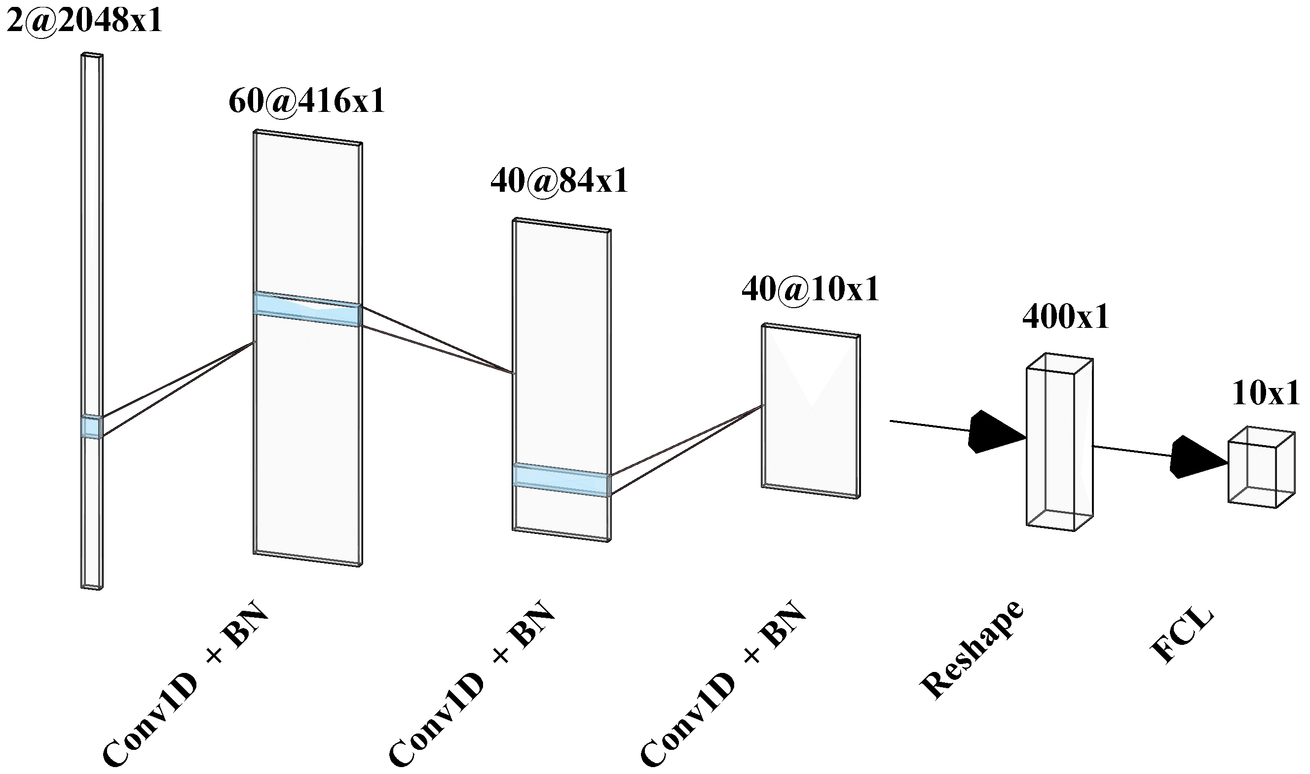
Figure 1. Convolutional layer computation composed in the matrix multiplication form visualised over two non-overlapping local areas and two channels.
Applsci 12 04411 g001
Figure 2. Feature maps of the Ince’s model employed in this study. These feature maps correspond to a model that diagnoses the probability of 10 health states from vibration data measured with two vibration sensors.
Applsci 12 04411 g002
Figure 3. Feature maps of the WDCNN employed in this study. These feature maps correspond to a model that diagnoses the probability of 10 health states from vibration data measured with two vibration sensors.
Applsci 12 04411 g003
Figure 4. Feature maps of the SRDCNN employed in this study. These feature maps correspond to a model that diagnoses the probability of 10 health states from vibration data measured with two vibration sensors.
Applsci 12 04411 g004
Figure 5. Time series sample consisting of two input signals divided to overlapping training samples.
Applsci 12 04411 g005
Figure 6. Bearing fault test rig [33].
Applsci 12 04411 g006
Figure 7. Means and standard deviations of the accuracies of the baseline models with BN (red) and the same models with ND (green) on six different load domain shift problems over ten trial runs. The models diagnosed the bearing health state from the drive-end sensor data. The test data was drawn from the motor load domains the arrows point and the training data was drawn from the motor load domains the arrows point from.
Applsci 12 04411 g007
Figure 8. Means and standard deviations of the accuracies of the baseline models with BN (red) and the same models with ND (green) on six different load domain shift problems over ten trial runs. The models diagnosed the bearing health state from the drive-end and the fan-end sensors simultaneously. The test data was drawn from the motor load domains the arrows point and the training data was drawn from the motor load domains the arrows point from.
Applsci 12 04411 g008
Figure 9. Thruster rotating speed varied between the acquired vibration samples in the range between 100 RPM and 750 RPM.
Applsci 12 04411 g009
Figure 10. The azimuth thruster vibration was measured with an accelerometer sensor near the input shaft. The positions of the sensor and the faulty components are pointed with red lines.
Applsci 12 04411 g010
Figure 11. Mean and standard deviation of accuracies of the baseline models with BN (red) and the modified models with ND (green) on both binary fault detection problems over 10 trial runs. Datasets were randomly drawn for each trial separately. Every model was tested with the same randomly drawn set of samples.
Applsci 12 04411 g011
Table 1. Ince’s model architecture.
LayerKernel SizeChannels inFiltersStridePadding
Conv1D9 × 11 or 260518
Conv1D9 × 1604054
Conv1D9 × 1404093
FCL1×14001 or 10N/AN/A
Table 2. WDCNN architecture.
LayerKernel SizeChannels inFiltersStridePadding
Conv1D64 × 11 or 2161624
Conv1D3 × 1163211
Conv1D3 × 1326411
Conv1D3 × 1646411
Conv1D3 × 1646411
FCL1×119218N/AN/A
FCL1×1181 or 10N/AN/A
Table 3. SRDCNN architecture.
LayerKernel SizeChannels inFiltersStridePaddingDilation
RDConv1D64 × 11 or 2322311
RDConv1D32 × 132322312
RDConv1D16 × 132642304
RDConv1D8 × 164642288
RDConv1D4 × 1646422416
FCL1×14096100N/AN/AN/A
FCL1×11001 or 10N/AN/AN/A
Table 4. Number of training and test samples per bearing health state and motor load.
LoadSplitHB L B M B H I L I M I H O L O M O H
1 hpTrain
Test
1980
59
1980
59
1980
59
1980
59
1980
59
1980
59
1980
59
1980
59
1980
59
1980
59
2 hpTrain
Test
1980
59
1980
59
1980
59
1980
59
1980
59
1980
59
1980
59
1980
59
1980
59
1980
59
3 hpTrain
Test
1980
59
1980
59
1980
59
1980
59
1980
59
1980
59
1980
59
1980
59
1980
59
1980
59
Table 5. Azimuth thruster dataset statistics.
ThrusterConditionBG
1Healthy
Faulty
263
468
283
448
2Healthy
Faulty
108
843
200
751
3Healthy
Faulty
125
405
216
314
TotalHealthy
Faulty
496
1716
699
1513
Data
splits
Train
Val
Test
48,230
11,960
368
77,740
19,110
592
Publisher’s Note: MDPI stays neutral with regard to jurisdictional claims in published maps and institutional affiliations.

