Efficient Open-Set Recognition for Interference Signals Based on Convolutional Prototype Learning

Abstract

Interference classification plays an important role in anti-jamming communication. Although the existing interference signal recognition methods based on deep learning have a higher accuracy than traditional methods, these have poor robustness while rejecting interference signals of unknown classes in interference open-set recognition (OSR). To ensure the classification accuracy of the known classes and the rejection rate of the unknown classes in interference OSR, we propose a new hollow convolution prototype learning (HCPL) in which the inner-dot-based cross-entropy loss (ICE) and the center loss are used to update prototypes to the periphery of the feature space so that the internal space is left for the unknown class samples, and the radius loss is used to reduce the impact of the prototype norm on the rejection rate of unknown classes. Then, a hybrid attention and feature reuse net (HAFRNet) for interference signal classification was designed, which contains a feature reuse structure and hybrid domain attention module (HDAM). A feature reuse structure is a simple DenseNet structure without a transition layer. An HDAM can recalibrate both time-wise and channel-wise feature responses by constructing a global attention matrix automatically. We also carried out simulation experiments on nine interference types, which include single-tone jamming, multitone jamming, periodic Gaussian pulse jamming, frequency hopping jamming, linear sweeping frequency jamming, second sweeping frequency jamming, BPSK modulation jamming, noise frequency modulation jamming and QPSK modulation jamming. The simulation results show that the proposed method has considerable classification accuracy of the known classes and rejection performance of the unknown classes. When the JNR is −10 dB, the classification accuracy of the known classes of the proposed method is 2–7% higher than other algorithms under different openness. When the openness is 0.030, the unknown class rejection performance plateau of the proposed method reaches 0.9883, while GCPL is 0.9403 and CG-Encoder is 0.9869; when the openness is 0.397, the proposed method is more than 0.89, while GCPL is 0.8102 and CG-Encoder is 0.9088. However, the rejection performance of unknown classes of CG-Encoder is much worse than that of the proposed method under low JNR. In addition, the proposed method requires less storage resources and has a lower computational complexity than CG-Encoder.

1. Introduction

With the rapid development of wireless communication technology and the increasing of electronic equipment, the electromagnetic environment is becoming more and more complex. In the future, the communication system will face more kinds of multi-source and multi-mode interference [1]. Adopting corresponding anti-interference measures according to the identified interference signals can effectively improve the communication quality. Therefore, communication interference recognition will be one of the key technologies of intelligent anti-interference communication in the future and has attracted the attention of many researchers.

Most of the traditional interference recognition methods are composed of feature extraction and pattern recognition. The feature extraction module uses a signal high-order cumulant [2], signal space [3,4] and transform domain [5,6,7] to complete the signal features extraction. The pattern recognition module uses a decision tree, SVM, BP neural network and other methods in traditional machine learning to complete the interference class decisions. However, the performance of such methods depends on the rationality of the feature selection, which is related to the cognition of professionals toward interference signals, so human factors have great influence. In addition, the traditional interference recognition methods also have problems such as low recognition accuracy. With the development of deep learning, more and more interference recognition algorithms based on deep learning and convolutional neural networks (CNN) have been proposed [8,9,10,11,12,13,14]. Datasets produced by simple signal preprocessing can be used to obtain a very high recognition accuracy [15], which solves the problem of feature parameters selected artificially in traditional methods. However, the above recognition methods based on deep learning have a closed hypothesis, which is called closed-set recognition (CSR), i.e., the types of interference signals in the test phase appeared in the training phase. When a new type of interference appears, the existing methods will identify it incorrectly as one of the known types. Since the communication interference may be the malicious electromagnetic signals transmitted by non-partners, with the rapid development of science and technology, new interference will emerge continually and cannot be known in advance [1]. Therefore, the open-set recognition (OSR) of interference signals needs to be solved urgently. There have been few OSR works for wireless signals [1,16,17,18,19]. Refs. [1,16] decoupled the known classes classification and the unknown classes rejection, which have good OSR performance under the background of low noise power, but their OSR performance decreases significantly under the background of high noise power. References [17,18,19] employed different methods to generate “fake” unknown class signals, which are used to train a network with known class signals together. However, their performance strongly depends on the “fake” unknown class signals.

Recently, prototype learning methods have been used for OSR because of their high intraclass compactness and interclass separability of sample features and achieved good performance [20,21,22]. However, these methods cannot be directly applied to the OSR of noisy interference signals. Therefore, this paper proposes an OSR classifier for interference signals based on convolution prototype learning.

The contributions of this paper are mainly as follows:

• We propose a new hollow convolution prototype learning (HCPL). A new hybrid loss function is designed that includes an inner-dot-based cross-entropy (ICE) loss, center loss (CL) and radius loss, to make the features of the known class signals at the periphery of the feature space;
• We propose a model that is used for the OSR of interference signals and called hybrid attention and feature reuse net (HAFRNet), which contains a feature reuse structure and hybrid domain attention module (HDAM);
• The influence of the hyperparameter in the hybrid loss function of HCPL is analyzed, and the role of HDAM and the feature reuse structure in the OSR of interference signals is proven in a simulation. The OSR experimental results of nine common interference types show that the proposed method has a better performance and less parameters than other methods under different openness.

The rest of this paper is organized as follows. Section 2 presents related works. Section 3 models the OSR problem of the interference signals. Section 4 discusses the proposed method in detail. Section 5 gives the simulation results and analyzes the performances of different methods in detail. Lastly, Section 6 concludes this paper and discusses our future work.

2. Related Work

2.1. Interference Signal Recognition Based on Deep Learning

To solve the problem of feature parameters selected artificially and the poor recognition accuracy in traditional jamming recognition methods, many works based on deep learning have been carried out. Since the convolution kernel of CNN is similar to the filter in traditional signal processing, a lot of recognition methods based on deep learning use CNN to extract features [8,9,10,11,12,23]. CNN was used to recognize jamming signals [8,9], and the network input was short-time Fourier transform (STFT) data of jamming signals [8] and time–frequency maps of simulated jamming signals [9], respectively. JRNet was proposed to recognize ten kinds of suppression jamming signals in [10], which was based on power spectrum features. The CNN-based Siamese network realized radar jamming signal recognition, which deals with the issue of limited training samples [11]. The AC-VAEGAN network structure solved the performance deterioration of the communication jamming recognition method in the case of a small sample set [12]. The Auto-Encoder network built by stacking LSTM reconstructed the transmitted signal, and another RNN realized a separated interference signal recognition in [13]. Multilayer perceptron was used to recognize jamming signals whose input is a singular value of the signal matrix [14]. However, these methods are closed-set recognition. Different from the above works, in this paper, the open-set recognition method of interference signals based on convolution prototype learning is presented.

2.2. Open-Set Recognition

OSR is to identify the known class samples seen during the training phase and reject the unknown class samples not seen in the training phase, i.e., to achieve high unknown class performance rejection and to keep excellent known classes recognition performances. Therefore, it is necessary to design a special model for the OSR problem [24,25,26,27,28,29,30]. OpenMax [24] used Weibull-based calibration to augment the Softmax layer of a deep classifier, but its OSR performance is poor. A competitive overcompleted output layer (COOL) neural network [25] was proposed to avoid overgeneralization over regions far from the training data. OSRCI [26] used GAN to generate “fake” unknown class samples, which are closed to known class samples but do not belong to a known class, to assist in network training. In Refs. [27,28], the OSR performance of the network was further enhanced by modifying the model based on OSRCI. The authors in [29] constructed faithful unknown class samples based on a generative causal model, decoupled the internal relationship between sample features and category features by designing a special loss function and obtained a better image OSR performance. OpenGAN [30] obtained outlier data according to outlier exposure [31] and selected the discrimination model with the optimal performance by using outlier data, which solved the problem of unstable training of GAN in the OSR. Although, to some extent, combining GAN can improve the OSR ability in image classification, the quality of “fake” interference signals with additive noise generated by GAN is not high, so it even reduces the OSR performance for interference signals.

The above works are all advanced research for image open-set recognition. For open-set recognition of wireless signals, some works have also been carried out [1,16,17,18,19]. The authors in [16] used a classification task and signal reconstruction task to jointly train the feature extractor and used another Siamese network to realize the OSR of radio frequency fingerprinting. However, multiple networks make the process very complicated. Conditional VAE was used to generate “fake” unknown classes signal in [17], while boundary known class signals were used to imitate unknown class signals in [18], but their performance depends on the quality of “fake” unknown class signals. Multi-task learning was used to get better feature representation, and CountGAN was used to generate “fake” unknown classes according to known boundary class signals in [19], but it needs more priori information to carry out multi-task learning, and the quality of the generated signal is still an important role affecting the performance. Combined with VAE and CGDL [32], CG-Encoder was proposed in [1] to realize the OSR of interference signals. It has an excellent unknown class rejection performance under a high jamming–noise ratio (JNR), but its anti-noise ability is poor, i.e., its performance decreases significantly under a low JNR. The proposed method in this paper can achieve a high OSR performance of interference signals even under a low JNR.

2.3. Prototype Learning

Prototype learning belongs to metric learning. It is a clustering algorithm derived from the KNN classifier. Different from unsupervised clustering algorithms, prototype learning uses the supervised information of samples to cluster in the training phase and learns a group of N-dimensional prototypes $\{P_1,P_2,P_3\dots \}$ as cluster centers. The training procedure of prototype learning is composed of feature extractors and prototype updating. The deep prototype learning has a powerful automatic feature extraction ability and end-to-end updating policy, so it has a better performance than the traditional prototype learning [20,21,22,33]. In Ref. [33], the center loss was used as the regularization term for the cross-entropy loss to reduce the Euclidean distance between similar samples to obtain stronger intraclass compactness, and the network parameters were jointly trained with the prototype to find a more suitable embedding feature space and prototypes. To realize the OSR, the cross-entropy loss in [33] was modified to the Tuplet loss based on distance in [20], while it was replaced with distance-based cross-entropy loss (DCE), one-vs-all loss (OVA) and prototype loss in [21,22], which further improved the intraclass compactness and interclass separability. However, because the known class sample features overlapped the unknown class sample features in the interior of the feature space, the OSR performance of prototype learning is limited. To solve this problem, we propose hollow convolutional prototype learning with a new hybrid loss function, which clusters known class signal features to the periphery of the feature space.

3. The Model of OSR of Interference Signals

The OSR of interference signals means that, during the testing phase, the classifier can not only classify the known interference signal (KIS) but also reject the unknown interference signal (UIS), which does not appear in the training stage, i.e., to avoid the UIS being incorrectly classified as one of the known classes.

A training dataset $\{(x_1,y_1),\dots ,(x_n,y_n)\}$, including $n$-labeled KISs, and a test dataset $\{t_1,\dots ,t_u\}$, including $u$-unlabeled samples, are given, where $y_i\in \{1,\dots ,N\}$ is the label of sample $x_1$ and $N$ is the number of known classes. In the OSR problem, test sample $t_i$ may belong to either a known class $\{1,\dots ,N\}$ or unknown class $\{N+1,\dots ,N+U\}$, where $U$ is the number of unknown classes in the testing phase.

The interference signal is embedded into the feature space through a feature extractor. All KISs are embedded in the closed space, and the space far from all KISs is called the open space. From the problem description, the OSR of the interference signals can be decoupled into closed-set multiclassification and open-set binary classification.

For closed-set multiclassification, labeling any KIS as the wrong class brings risk, and it can be defined as an empirical risk $R_e$:

$$R_e={\displaystyle {\int }_C{g}_e(x,y)dx}$$

(1)

where $g_e(·,·)$ is a recognition function for closed-set multi-classification. $g_e(x,y)=0$ indicates that the KIS is classified correctly, while $g_e(x,y)=1$ indicates that $x$ is classified erroneously.

For the open-set binary classification, labeling any UIS as any class incurs risk, which is defined as the open space risk $R_o$ [34]:

$$R_o=\frac{{\displaystyle {\int }_O{g}_o(x)dx}}{{\displaystyle {\int }_{C\cup O}{g}_o(x)dx}}$$

(2)

where $g_o(·)$ is a measurable recognition function for open-set binary classification. $g_o(x)=1$ indicates that the sample $x$ is recognized as KIS; otherwise, $g_o(x)=0$. Therefore, open space risk is considered as a relative measure of open space compared to the overall measure space.

Then, the goal of the OSR of interference signals is to find two suitable recognition functions, $g_e(·,·)$ and $g_o(·)$, to minimize the joint risk, which is composed of empirical risk and open space risk:

$$\underset{g_e(·,·),g_o(·)}{\arg \min }\{R_e+\lambda R_o\}$$

(3)

where $\lambda$ is a regularization constant.

4. Proposed Method

Hollow convolutional prototype learning for interference OSR is composed of a feature exactor and a prototype classifier, as shown in Figure 1. The feature exactor $f(·;\theta )$ transforms the input $x$ to d-dimensional deep feature representation, where $\theta$ denotes the parameters in the feature extractor. The prototype classifier $C(·;M)$ consists of prototypes $\left\{{\mathit{m}}_{ij}\right|j\in \{1,\dots ,J\}\}$ corresponding to each class $i\in \{1,\dots ,N\}$, and the label is assigned to the input $x$ according to the nearest prototype, where $M$ is the set of all prototypes, and $J$ is the number of prototypes for each class. Below, we maintain one prototype for each class by default [22]. The way of HCPL to realize interference OSR is to convert the similarity between the signal features and prototypes into probability and to judge whether a signal is a KIS through the threshold in the prototype classifier.

Below, we introduce HCPL from two phases. In the inference phase, we propose a feature extractor that uses HAFRNet and a prototype classifier based on similarities. In the training phase, we design a hybrid loss function to update the parameters of the feature extractor and prototypes.

4.1. Feature Extractor and Prototype Classifier

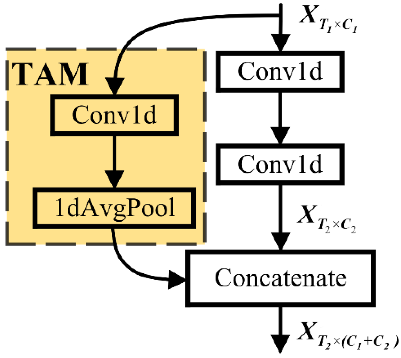
4.1.1. Feature Reuse Structure

The increase of the number of network layers will strengthen the feature extraction ability of the feature extractor, but a degradation problem may be exposed [35], i.e., the performance of a deep network is lower than that of a shallow network. To avoid the problem, we propose a feature reuse structure, which is modified by a simplified version of a DenseNet structure [36]—that is, the version without the transition layer. Since the interference signal is a one-dimensional sequence, we use a one-dimensional convolution kernel to replace the 2D convolution kernel in the original DenseNet, and the feature reuse structure is shown in Figure 2.

Conv1d represents a one-dimensional convolutional layer. The $Y\times 1$ convolution operation can be expressed as:

$${\mathit{X}}^{out}(t,c)={\displaystyle \sum _{i=-\frac{Y-1}{2}}^{\frac{Y-1}{2}}{\displaystyle \sum _{j=0}^{Ch-1}{G}_{i,j,c}\times {\mathit{X}}^{in}(t\times s+i,j)}}$$

(4)

where $G_{i,j,c}$ represents the weights of the $c$-th convolution kernel, ${\mathit{X}}^{out}(t,c)$ and ${\mathit{X}}^{in}(t,c)$ represent the convolution output and input of the corresponding position, $Ch$ is the channel number of ${\mathit{X}}^{out}(t,c)$ and $s$ is the stride of the convolution kernel.

1dAvgPool represents a one-dimensional average pooling layer, and its operation can be expressed as:

$${\mathit{X}}^{out}(t,c)=\frac{1}{Pn}{\displaystyle \sum _{i=0}^{Pn-1}{\mathit{X}}^{in}(t\times s+i,c)}$$

(5)

where $Pn$ is the size of pooling kernel and $s$ is the stride of the convolution kernel.

${\mathit{X}}_{T_1\times C_1}$ indicates the input feature map, which has $T_1$ time points and $C_1$ channels. ${\mathit{X}}_{T_2\times C_2}$ indicates the middle feature map, which is obtained from ${\mathit{X}}_{T_1\times C_1}$ passing through two convolution layers.

The input feature map ${\mathit{X}}_{T_1\times C_1}$ should be aligned with ${\mathit{X}}_{T_2\times C_2}$ in the time domain by a time alignment module (TAM) when $T_1\ne T_2$, and then, ${\mathit{X}}_{T_1\times C_1}$ and ${\mathit{X}}_{T_2\times C_2}$ are implemented channel-wise concatenation to get the output feature map ${\mathit{X}}_{T_2\times (C_1+C_2)}$. The TAM is composed of a one-dimensional convolution layer and one-dimensional average pooling layer, and the number of input and output channels of the TAM is the same.

The subscript dimension of the feature map is omitted below for simplicity.

On the one hand, because the shallow features are directly connected to the final classifier like the deep features in the feature reuse structure, supervision information can be provided by the shallow layers directly, and the middle layers are forced to learn usable features [36]. On the other hand, feature reuse can greatly reduce the number of parameters without performance deterioration.

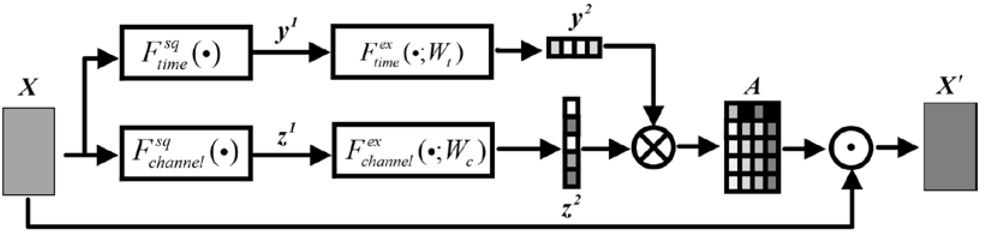
4.1.2. Hybrid Domain Attention Module

SENet [37] applies the idea of an attention mechanism to the CNN to recalibrate channel-wise feature responses by explicitly modeling interdependencies between channels adaptively. However, in 1DCNN, except the channels, different time points should also be given different attention. Therefore, we propose a hybrid domain attention module (HDAM) to recalibrate the time-wise and channel-wise feature responses by constructing a global attention matrix automatically. The HDAM structure is shown in Figure 3, which recalibrates two domains while the SENet recalibrates one domain, i.e., channel-wise.

$\mathit{X}$ is the input feature map of HDAM, $\mathit{A}$ is the global attention weight matrix, ${\mathit{X}}^{\prime }$ is the output feature map of HDAM and their elements are $\mathit{X}(t,c)$, $\mathit{A}(t,c)$ and ${\mathit{X}}^{\prime }(t,c)$, respectively.

First, to get time-wise and channel-wise statistics, the HDAM adopts time-wise and channel-wise global average pooling for the feature map, as shown in Equations (6) and (7):

$${\mathbf{y}}^{\mathbf{1}}=F_{time}^{sq}(\mathit{X})=\frac{1}{C}{\displaystyle \sum _{c=1}^C\mathit{X}(:,c)}$$

(6)

$${\mathbf{z}}^{\mathbf{1}}=F_{channel}^{sq}(\mathit{X})=\frac{1}{T}{\displaystyle \sum _{t=1}^T\mathit{X}(t,:)}$$

(7)

where $F_{channel}^{sq}(·)$, $F_{time}^{sq}(·)$, ${\mathbf{y}}^{\mathbf{1}}$ and ${\mathbf{z}}^{\mathbf{1}}$ indicate the time-wise global average pooling function, channel-wise global average pooling function, time-wise statistics and channel-wise statistics, respectively.

Then, two bottlenecks with two fully connected (FC) layers are used to learn time-wise and channel-wise dependencies automatically, and one-dimensional attention weight vectors are obtained as follows:

$${\mathbf{y}}^{\mathbf{2}}=F_{time}^{ex}({\mathbf{y}}^{\mathbf{1}};W_t)=\sigma (\delta ({\mathbf{y}}^{\mathbf{1}}{W}_t^1)W_t^2)$$

(8)

$${\mathbf{z}}^{\mathbf{2}}=F_{channel}^{ex}({\mathbf{z}}^{\mathbf{1}};W_c)=\sigma (W_c^2\delta (W_c^1{\mathbf{z}}^{\mathbf{1}}))$$

(9)

where $F_{time}^{ex}(·)$, $F_{channel}^{ex}(·)$, ${\mathbf{y}}^{\mathbf{2}}$ and ${\mathbf{z}}^{\mathbf{2}}$ indicate a time-wise bottleneck, channel-wise bottleneck, time-wise attention weight vector and channel-wise attention weight vector, respectively. $\delta (·)$ refers to the ReLu function, $W_t^1\in {ℝ}^{C\times \frac{C}{q}}$, $W_t^2\in {ℝ}^{\frac{C}{q}\times C}$, $W_c^1\in {ℝ}^{\frac{T}{q}\times T}$, $W_c^2\in {ℝ}^{T\times \frac{T}{q}}$ and $q$ is the compression rate. Using a one-shot activation function will lead to the feature of only one channel and one time position being emphasized, while the rest of the features are suppressed, so $\sigma (·)$ should be a sigmoid function, which controls the magnitude of the attention weight vector units. Note that ${\mathbf{y}}^{\mathbf{1}}$ and ${\mathbf{y}}^{\mathbf{2}}$ are row vectors, while ${\mathbf{z}}^{\mathbf{1}}$ and ${\mathbf{z}}^{\mathbf{2}}$ are column vectors.

The global attention weight matrix $\mathit{A}$ is obtained by multiplying ${\mathbf{y}}^{\mathbf{2}}$ and ${\mathbf{z}}^{\mathbf{2}}$:

$$\mathit{A}={\mathbf{z}}^{\mathbf{2}}{\mathbf{y}}^{\mathbf{2}}$$

(10)

Specifically, $\mathit{A}(t,c)$ indicates how much attention should be paid to the data of time point $t$ of the $c$-th channel.

Finally, the recalibrated output feature map ${\mathit{X}}^{\prime }$ is obtained by element-wise multiplying $\mathit{A}$ and $\mathit{X}$:

$${\mathit{X}}^{\prime }=\mathit{A}\odot \mathit{X}$$

(11)

where $\odot$ is the Hadamard product.

Since the receptive fields of the convolution kernel of the CNN are local, each unit of the feature map cannot exploit the contextual feature information outside of the corresponding time window. However, the HDAM can aggregate the global information in the pooling stage of the channel domain and the dependent learning stage of the time domain, so that all units can obtain the information outside the time window in the middle layer, unlike a traditional CNN, which needs to wait until the last fully connection layer to aggregate information.

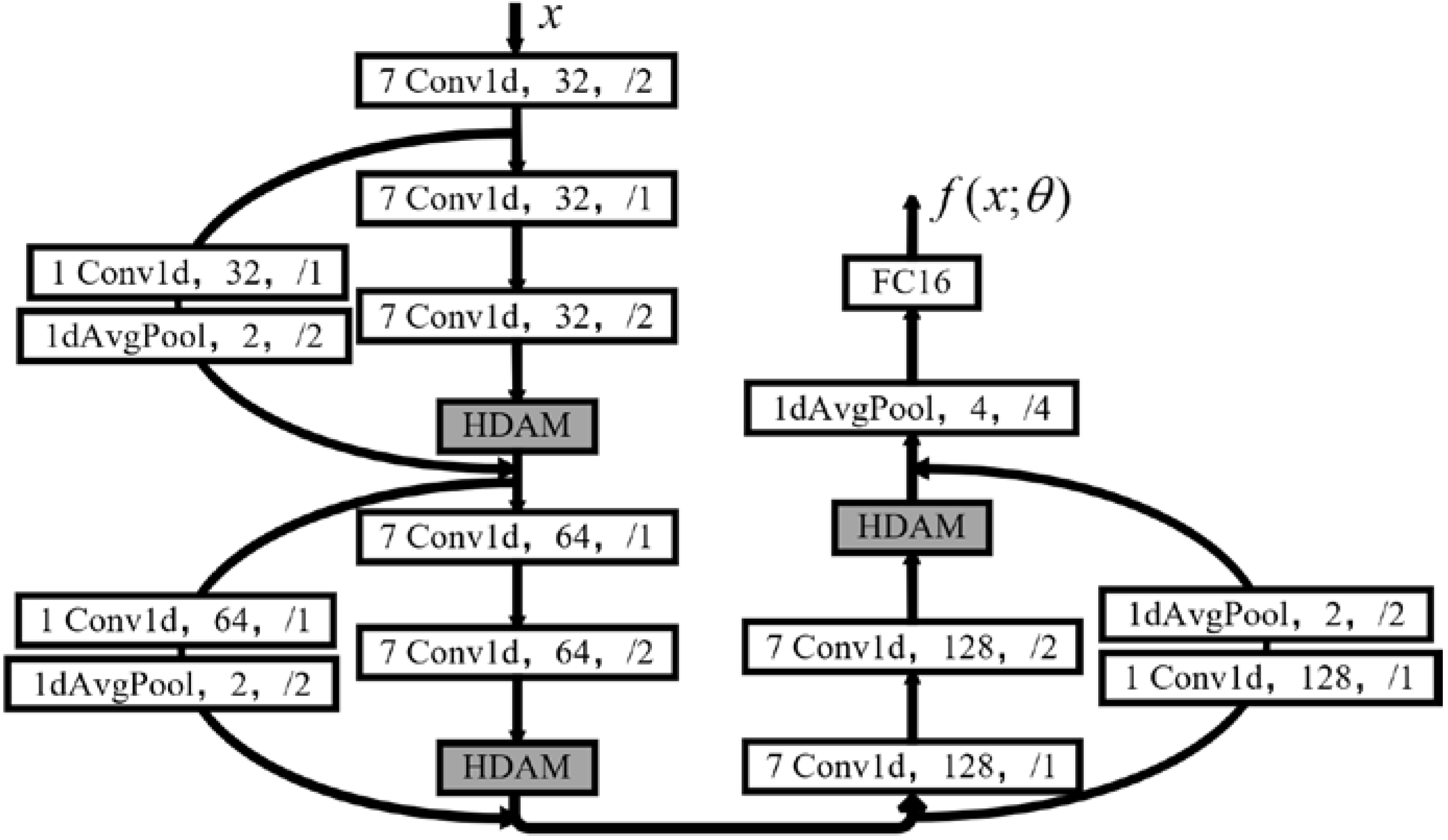
4.1.3. Hybrid Attention and Feature Reuse Net

Combining with the feature reuse structure and hybrid attention module, the proposed feature exactor for interference signals, i.e., HAFRNet, is shown in Figure 4.

HAFRNet consists of ten one-dimensional convolution layers, three HDAMs, four one-dimensional average pooling layers and one FC layer. For simplicity, we did not draw the BatchNormlization layer and ReLu layer before each convolution layer in Figure 4, which can be defined as Equations (12) and (13), respectively.

$$BN(x)=a\frac{x-{\mu }_B}{\sqrt{{\sigma }_B^2+\epsilon }}+b$$

(12)

$$\mathrm{ReLu}(x)=\max (0,x)$$

(13)

where ${\mu }_B$ and ${\sigma }_B$ are the mean and variance of the samples in the mini-batch, respectively, $a$ and $b$ are learnable parameters and $\epsilon$ is a small constant added to the mini-batch variance for numerical stability.

The input of HAFRNet is a one-dimensional noisy interference signal, $x$, while its output is a 16-dimensional feature representation. The shortcut in Figure 4 is the feature reuse structure, as shown in Figure 2, which is a channel-wise concatenation. The convolution layer parameter meanings are the size, type, number and stride of the convolution kernel, respectively. For example, {7 conv1d, 32, /2} means the convolution layer uses one-dimensional convolution with 32 convolution kernels whose size is 7 × 1 and stride is 2. The average pooling layer parameter meanings are the type, size and stride of the pooling kernel, respectively. For example, {1dAvgPool, 4, /2} means the average pooling layer uses one-dimensional average pooling with a pooling kernel whose size is 4 × 1, and the stride is 2. The compression rate of the HDAM is 8. The FC layer parameter is the number of neurons in the output layer.

4.1.4. Prototype Classifier

KIS classification and UIS rejection are realized by using a prototype classifier after feature extraction in the HCPL.

The multiclassification process in the prototype classifier is formulated as:

$$x\in class\arg \underset{i=1}{\overset{N}{\max }}S({\mathit{m}}_i;f(x;\theta ))$$

(14)

where $f(x;\theta )$ is the feature of sample $x$, and $S({\mathit{m}}_i,f(x;\theta ))$ is the similarity measure function defined as the inner product between the sample feature and prototypes as follows:

$$S({\mathit{m}}_i;f(x;\theta ))=f^{{\rm T}}(x;\theta ){\mathit{m}}_i$$

(15)

To realize the OSR of interference signals, we propose a process for KIS classification and UIS rejection according to the inner product between the sample feature and each prototype, as shown in Figure 5.

For each test sample $x$, the probability score of class $i$ based on the inner product is defined as:

$$scor{e}^i=\frac{e^{\alpha f^{\mathrm{T}}(x;\theta )·{\mathit{m}}_i}}{{\displaystyle \sum _{k=1}^N{e}^{\alpha f^{\mathrm{T}}(x;\theta )·{\mathit{m}}_k}}}$$

(16)

where $\alpha$ is a hyper-parameter that controls the hardness of the similarity–probability conversion.

When a threshold $\beta$ is given, the sample belongs to unknown classes if the highest probability score is lower than $\beta$; otherwise, it belongs to known classes:

$$prediction=\{\begin{array}{cc}class\arg \underset{i}{\max }scor{e}^i\hfill & if\underset{i}{\max }scor{e}^i>\beta \hfill \\ unknown\hfill & if\underset{i}{\max }scor{e}^i<\beta \hfill \end{array}$$

(17)

4.2. Hybrid Loss Function

As the core of convolutional prototype learning, the loss function used in the training phase will affect the distribution of the sample features in the feature space, which is related to the OSR performance. Therefore, two aspects are considered in the design of the loss function. On the one hand, it should decrease the distance between the sample features and the ground truth prototype and increase the distance between the sample features and other prototypes. On the other hand, the prototypes should be updated to the periphery of the feature space to avoid overlapping of the UIS and KIS features.

According to the principle of maximum entropy, for an unknown sample without any prior information, a well-trained classifier tends to assign known labels to it with equal probability, i.e., the classifier usually embeds an unknown sample feature into the inside of the feature space rather than random positions in the space [38,39]. However, because GCPL [21,22] uses DCE and OVA as the discriminative loss, the learned prototypes also appear in the interior of the feature space, and there is a lot of overlap between the UIS features and KIS features. Although replacing the Euclidean distance of GCPL with the cosine distance can make KIS features distribute all over the hypersphere, the unknown class will also be assigned to the hypersphere in the test phase, which does not solve the overlap problem. To deal with this issue, the HCPL adopts an inner product-based loss function as the discriminative loss to update the prototypes to the periphery of the feature space. The feature space of the visual comparison of the HCPL and GCPL will be seen in Section 5.

To update all prototypes per iteration, the Softmax function is used to normalize the similarity to the probability:

$$p(x\in y|x)=\frac{e^{\alpha f^{\mathrm{T}}(x;\theta ){\mathit{m}}_y}}{{\displaystyle \sum _{i=1}^N{e}^{\alpha f^{\mathrm{T}}(x;\theta ){\mathit{m}}_i}}}$$

(18)

For the training sample $(x,y)$, the inner-dot-based cross-entropy loss (ICE) is designed:

$$L_d=-\ln p(x\in {\mathit{m}}_y|x)$$

(19)

According to the model of OSR of the interference signals, ICE can be considered as an empirical risk. Reducing ICE will essentially increase the similarity of the sample features to the ground truth prototype and decrease the similarity to others. By minimizing ICE, the network tends to distribute the prototypes corresponding to different classes uniformly on a hypersphere surface. However, if ICE is used only, it means only the empirical risk is considered in the OSR of the interference signals, and there are still many known class sample features in the interior of the feature space that does not provide enough open space for the UISs. Therefore, to constrain the KIS features to the periphery of the bounded feature space of the hypersphere and to reserve the interior of the feature space for the unknown classes, the center loss (CL) is considered as the open space risk and designed as Equation (20) to the improve intraclass compactness:

$$L_c={\Vert {\mathit{m}}_y-f(x;\theta )\Vert }_2^2$$

(20)

When ICE and CL are used together, ICE can also be regarded as having the ability to reduce the open space risk. Since ICE can keep prototypes away from the interior of the feature space and CL can enhance the intraclass compactness, KIS features are also kept away from the interior. Finally, the periphery of the hypersphere is considered as a closed space, while the interior is regarded as an open space.

Then, because the prototypes obtained by using the SGD algorithm in the training phase are not on the hypersphere completely, to avoid a low OSR performance due to a large prototype, the norm gaps radius loss (RL) is designed as follows:

$$L_r={({\Vert {\mathit{m}}_y\Vert }_2-r)}^2$$

(21)

where $r$ is the hypersphere radius that can be trained jointly with the feature extractor and prototypes.

Combined with ICE, CL and RL, the hybrid loss function is defined as:

$$L=L_d+{\lambda }_c{L}_c+{\lambda }_r{L}_r$$

(22)

where ${\lambda }_c$ and ${\lambda }_r$ are the regularization parameters of CL and RL, respectively.

The hybrid loss function is derivable with regards to $f(·;\theta )$, $\left\{{\mathit{m}}_i\right|i\in \{1,\dots ,N\}\}$ and $r$, so the derivatives can be calculated as:

$${\nabla }_{f}L={\displaystyle \sum _{i=1}^N{\mathit{m}}_{i}p(x\in {\mathit{m}}_i|x)-\alpha {\mathit{m}}_y+2{\lambda }_c(f(x;\theta )-{\mathit{m}}_y)}$$

(23)

$${\nabla }_{m_y}L=\alpha f(x;\theta )(p(y|x)-1)+2{\lambda }_c({\mathit{m}}_y-f(x;\theta ))+2{\lambda }_r\frac{{\mathit{m}}_y}{{\Vert {\mathit{m}}_y\Vert }_2}({\Vert {\mathit{m}}_y\Vert }_2-r)$$

(24)

$${\nabla }_{m_j}L=\alpha f(x;\theta )p(x\in {\mathit{m}}_j|x)$$

(25)

$${\nabla }_{r}L=-2{\lambda }_r({\Vert {\mathit{m}}_y\Vert }_2-r)$$

(26)

where ${\mathit{m}}_y$ is the ground truth prototype of training sample $x$ and ${\mathit{m}}_j$ is the others.

5. Performance Analysis

5.1. Simulation Setting

During training, the proposed methods use momentum SGD as the optimizer, whose momentum is 0.9 and initial learning rate is 0.01. The weight decay of all the optimizers is 1 × 10⁻⁴ and the step decay learning rate strategy is used as the learning rate schedule with 16 steps and a decay factor of 0.3. All models were trained for 200 epochs whose mini-batch size is 128 and tested on a computer with CPU Intel Core i7-9700K, running memory 32 GB and GPU GeForce RTX 2070Super.

5.1.1. Datasets

Nine kinds of interference signals, which include single-tone jamming, multitone jamming, periodic Gaussian pulse jamming, frequency hopping jamming, linear sweeping frequency jamming, second sweeping frequency jamming, BPSK modulation jamming, noise frequency modulation jamming and QPSK modulation jamming, are generated by matlabR2020a. The details of the parameters of each interference type are shown in

Table 1. Interference signals and their parameter settings.

Interference Types	Parameter Setting
Single-tone	The center frequency $f_c$ is between [100, 500] kHz, and the phase $\phi$ is between [0, 2π].
Multitone	The number $N$ of audio is [2, 10], and $f_c$, $\phi$ are the same as single-tone jamming.
Periodic Gaussian pulse	The pulse period $T$ is 2.5~10 μs, and the duty cycle is 1/8~1/2.
Frequency hopping	N = 20, {$f_c$} is between [100, 500] kHz, the frequency hopping period $T_h$ is between 3.2~6.4 μs, and the phase $\phi$ is between [0, 2π].
Linear sweeping frequency	The starting frequency $f_{c1}$ is [50, 100] kHz, and the ending frequency $f_{c2}$ is [300, 1000] kHz.
Second sweeping frequency	The frequency is quadratic, and other parameters are the same as linear sweeping frequency jamming.
BPSK modulation	The information symbol is a 32-bits 0,1 random sequence, the symbol period is 3.2 μs, and the modulation signal is sinusoidal signal.
Noise frequency	The frequency modulation coefficient is between [0.125, 0.933], and the carrier signal parameters are the same as single-tone jamming.
QPSK modulation	The information symbol is a 32-bit 0,1 random sequence, the symbol period is 3.2 μs, I-channel modulation signal is sinusoidal signal, Q-channel modulation signal is cosine signal.

. The sampling frequency is 10 MHz, and the number of sampling points is 1024. The added noise is additive white Gaussian noise, and the JNR ranges from −10 dB to 18 dB, with an interval of 2 dB. The number of data samples of each type per JNR is 1500, including 500 training samples, 500 verification samples and 500 test samples.

All datasets consist of the above nine interference signal types. Jamming-N is used to indicate that the dataset contains N known classes and 9-N unknown classes, which are randomly sampled and combined. During training, the input of the model is the known class samples. During testing, the input of the model is both the known class samples and unknown class samples, and the model must assign appropriate labels to the test samples of the known classes and reject the test samples of the unknown classes as the N + 1 class.

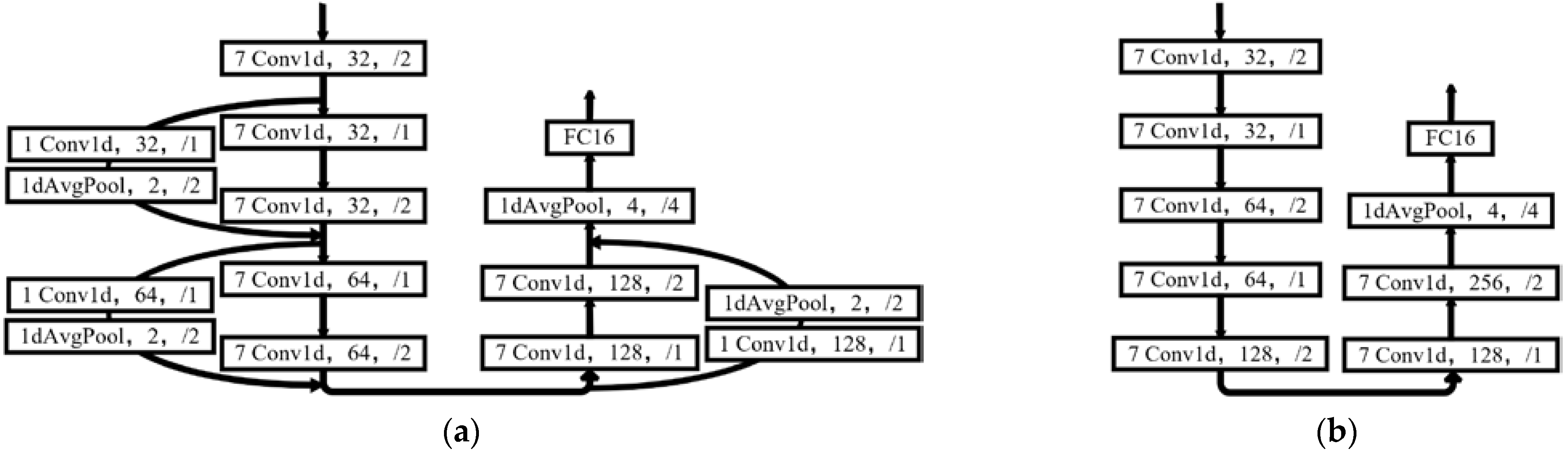
5.1.2. Structure of Feature Extractor

In order to illustrate the effectiveness of the HDAM and feature reuse structure, three feature extractors are used in HCPL, which are the HAFRNet shown in Figure 4, the feature reuse network (FRNet) shown in Figure 6a that uses only a feature reuse structure without HDAM and the CNN shown in Figure 6b. Therefore, the HCPL-HAFRNet (i.e., the proposed method), the HCPL-FRNet and the HCPL-CNN are denoted, respectively.

5.1.3. Performance Metrics

The unknown class rejection performance can be characterized by using the overall accuracy of the unknown class detection on a combined dataset of known class and unknown class samples. However, it is unknown in the testing phase how many samples from the unknown classes are in the real world, so it is not appropriate to compare the unknown class rejection performance of the methods using a (or set of) threshold.

AURoc [26], as a metric to measure the performance of a binary classification model, can be interpreted as the probability that a positive sample is assigned a higher score than a negative sample, which is a threshold-independent metric. Therefore, we use AURoc as the metric for the unknown class rejection performances of all methods.

An OSR method should not sacrifice the accuracy of closed-set classification while obtaining a better rejection performance of the unknown classes. Therefore, classification accuracy is used to evaluate the multiclassification performance of known classes. All experimental results in the following are averaged over six random experiments.

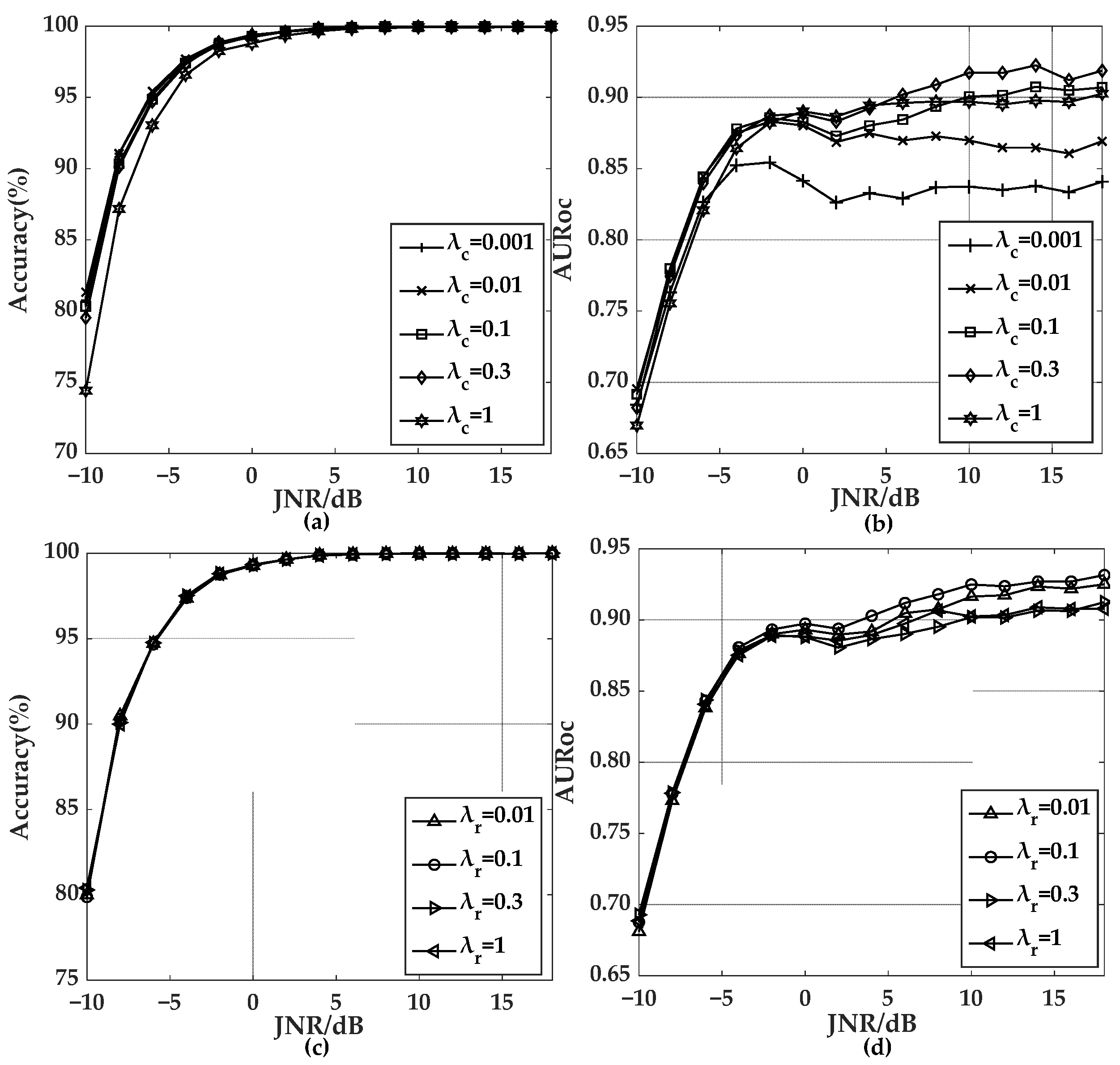
5.2. Effects of Hyperparameters of the Hybrid Loss Function

The hyperparameters ${\lambda }_c$ and ${\lambda }_r$ in the hybrid loss function directly affect the performance of HCPL. We carry out OSR experiments on the Jamming-7 dataset using HCPL-CNN. When ${\lambda }_r$ = 0, i.e., without using the prototype radius loss, the curves of the classification accuracy and AURoc with JNR under specific ${\lambda }_c$ are shown as Figure 7a,b, respectively. When ${\lambda }_c$ = 0.3, the curves of the classification accuracy and AURoc with JNR under specific ${\lambda }_r$ are shown as Figure 7c,d, respectively.

It can be seen from Figure 7a,b that the rejection performance of the unknown classes is improved greatly as ${\lambda }_c$ increases. However, when ${\lambda }_c$ is too large (${\lambda }_c$ = 1), the classification performance of the known classes at a low JNR, and the rejection performance of the unknown classes under various JNR decreases; this is because, when ${\lambda }_c$ becomes larger, the model increasingly focuses on the intraclass compactness of the features and ignores the interclass separability of the features. Therefore, ${\lambda }_c$ = 0.3 is chosen below.

As shown in Figure 7c,d, the prototype radius loss does not affect the classification performance of the known classes, while the rejection performance of the unknown classes increases first and then decreases with the increase of ${\lambda }_r$. Therefore, the prototype radius loss can improve the rejection performance of the unknown classes in HCPL, but when ${\lambda }_r$ is too large, the prototype radius loss cannot converge on the optimal value, resulting in a decrease of the rejection performance of the unknown classes. Therefore, ${\lambda }_r$ = 0.1 is chosen below.

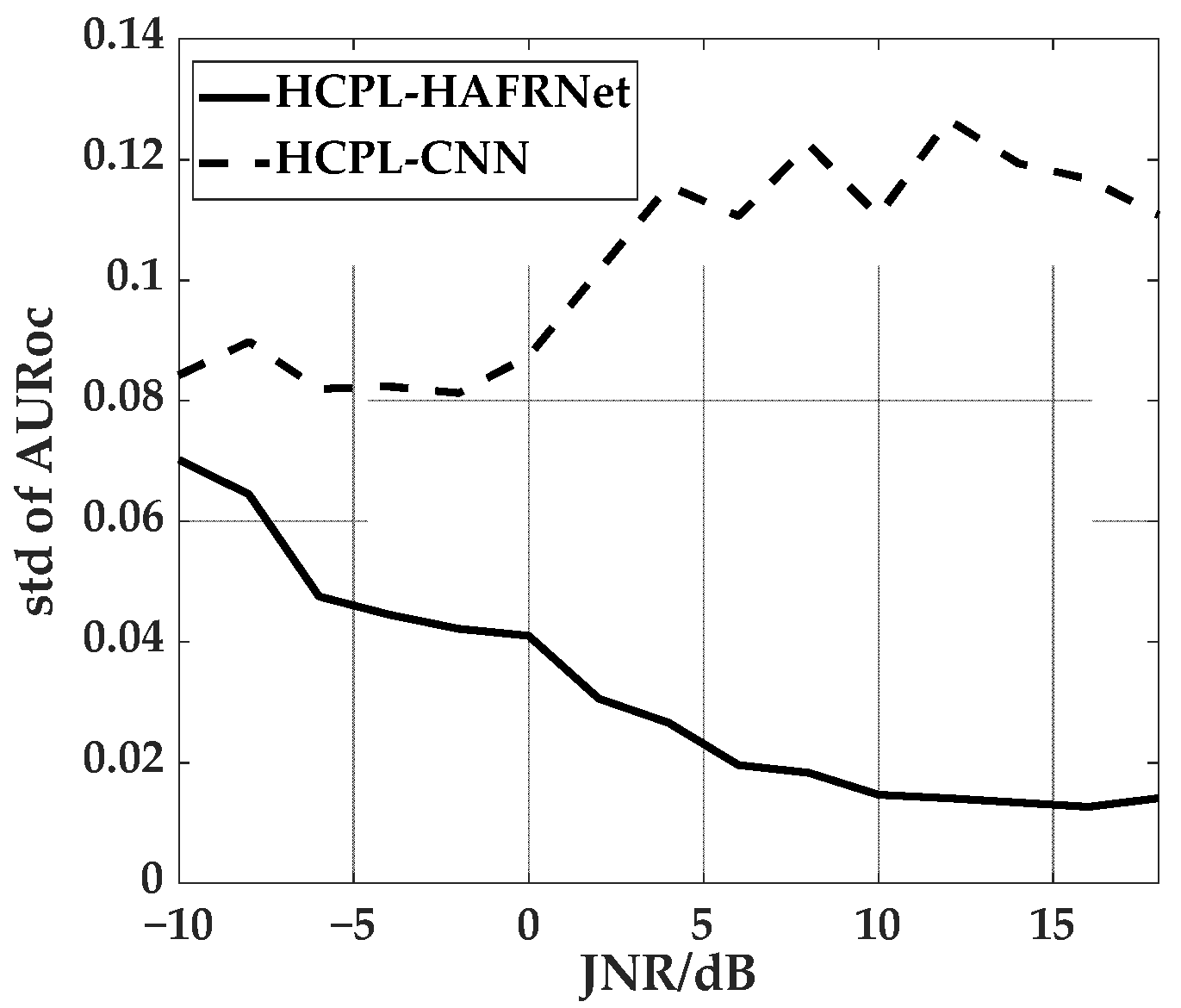
5.3. Effects of Feature Reuse Structure and HDAM

To investigate the effects of the feature reuse structure and HDAM on the OSR performance of HCPL, we carried out OSR experiments on the Jamming-7 dataset using HCPL-CNN, HCPL-FRNet and HCPL-HAFRNet, and the experimental results are shown in Figure 8. As seen in Figure 8a, HCPL-HAFRNet has the highest classification accuracy of the known classes, and the rest are too close to each other. When the JNR > 5 dB, the classification accuracy of all three algorithms for the known classes is close to 100%. Therefore, even with close-set multiclassification for interference signals, HAFRNet can improve the accuracy under low JNR while maintaining the accuracy under high JNR. As seen from Figure 8b, the HCPL-HAFRNet algorithm has the highest rejection performance of the unknown classes, and the other two are close. Hence, it can be seen that HDAM can improve the performances of both the known class classification and unknown class rejection.

The computational complexity and storage complexity of an algorithm are related to the number of the network parameters. The CNN has 518,768 parameters, and FRNet has 389,744 parameters, while HAFRNet has 416,624 parameters. Therefore, HAFRNet improves the performance of the known class classification and unknown class rejection at the same time while reducing the complexity compared with the CNN.

The dataset used in each experiment consists of known and unknown classes that are randomly sampled from nine interference signal classes and combined. Therefore, the rejection performance of the unknown classes in each random experiment using the same method is different because of the difference of the split of known and unknown classes. The variance of the AURoc is used to measure the effects of different partitions of known and unknown classes on the rejection performance of the unknown classes. We perform OSR experiments on the Jamming-7 dataset using HCPL-CNN and HCPL-HAFRNet. The results are shown in Figure 9. The variance of AURoc of HCPL-HAFRNet is much lower than that of HCPL-CNN under various JNR, and it decreases as JNR increases, while the variance of AURoc of HCPL-CNN increases as JNR increases. Therefore, the robustness of HCPL-HAFRNet in the unknown class rejection is much better than that of HCPL-CNN.

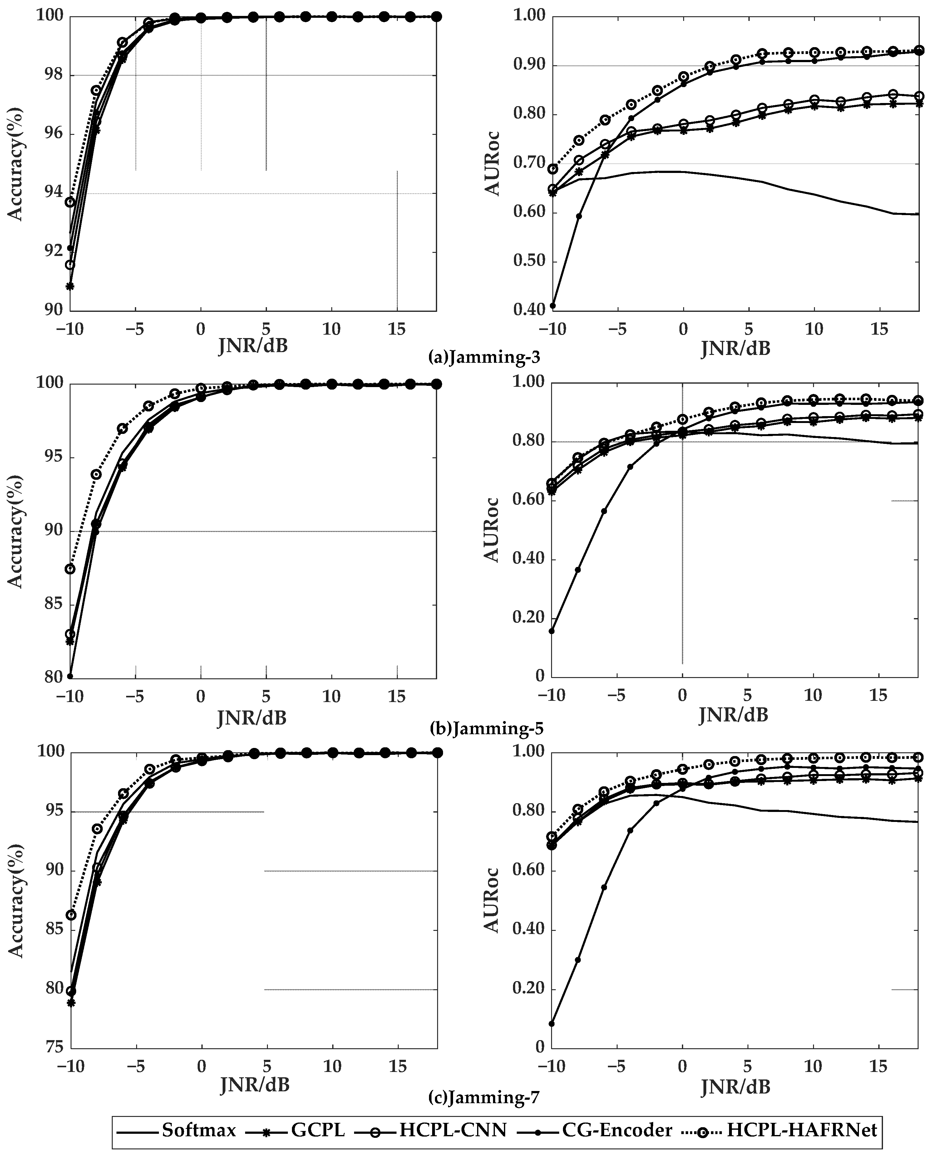
5.4. Comparison of Different Methods

The openness [35] of dataset Jamming-N is defined as:

$$Openess=1-\sqrt{\frac{2\times N}{N+K}}$$

(27)

where the total number of classes is $K$, and the known number of classes is $N$.

In this part, we compare the OSR performances of Softmax [26], GCPL [22], CG-Encoder [1], HCPL-CNN and HCPL-HAFRNet. Note that Softmax and GCPL use the CNN shown in Figure 6b as the feature extractor, and the training strategy follows the proposed method. Softmax has no hyperparameters in the loss function, while the weight parameters for the generative loss of GCPL is set as 0.1, which can get the best performance in the simulation through many parameter adjustment experiments. The network structure, parameter setting and training strategy of CG-Encoder are as follows [1]. The OSR experiments results of the above five algorithms on three different openness datasets: Jamming-3, Jamming-5 and Jamming-7 are shown in Figure 10.

As shown in the three diagrams of accuracy of Figure 10, HCPL-HAFRNet has the best classification accuracy of the known classes, which is 2–7% higher than the other methods under different openness and JNR = −10 dB, while the accuracy of the other methods is close, and all of them increase with the increase of the JNR. When the JNR is in the range of −10 dB to 5 dB, the accuracy of all five methods increases with the increase of the openness; this is because, when the total number of classes is fixed, the larger the openness is and the less the classification error source is. When JNR > 5 dB, the accuracy of all five methods is close to 100%.

It can be seen from the three diagrams of AURoc of Figure 10 that HCPL-HAFRNet has the best rejection performance of the unknown classes; this is because it uses the HDAM to enhance the information of critical time points and channels and ignore unimportant information. When JNR > 0 dB, the performance of CG-Encoder on different openness datasets is second only to that of HCPL-HAFRNet, but it is much worse than that of the other methods under low JNR. The HCPL-CNN performs better than GCPL under different openness and various JNR, because the HCPL-CNN constrains the closed space to a hypersphere, while all prototypes are on the hypersphere, i.e., sample features of the known classes are clustered far from the interior of the feature space and leaving space for the unknown classes. The GCPL outperforms Softmax, because it enhances the intraclass compactness and interclass separability of the sample features by prototype loss.

Except for Softmax, the performances of the remaining methods increase with the increase of JNR under different openness, and the performances are saturated when JNR > 5 dB. Therefore, when JNR is between 10 dB and 18 dB, the average AURoc is defined as the rejection performance plateau of the unknown classes, and the effect of openness on the performance plateau for the four methods is shown in

Table 2. Unknown class rejection performance plateau under the different openness of four methods. The best result in each Dataset is highlighted in bold.

Dataset (Openness)\Method	GCPL	CG-Encoder	HCPL-CNN	HCPL-HAFRNet
Jamming-2(0.397)	0.8102	0.9088	0.8132	0.8921
Jamming-3(0.293)	0.8197	0.9193	0.8346	0.9287
Jamming-4(0.216)	0.8409	0.9289	0.8677	0.9369
Jamming-5(0.155)	0.8774	0.9313	0.8888	0.9437
Jamming-6(0.106)	0.8854	0.9397	0.9071	0.9690
Jamming-7(0.065)	0.9093	0.9412	0.9268	0.9834
Jamming-8(0.030)	0.9403	0.9869	0.9710	0.9883

.

From Table 2, it can be seen that the rejection performance plateau of the HCPL-HAFRNet is higher than those of CG-Encoder under different openness, except for Jamming-2. The performance plateau of CG-Encoder is higher than those of the HCPL-CNN and GCPL, but the network of CG-Encoder has 7,259,881 parameters, which is more than 14 times HCPL-CNN and GCPL. Besides that, the rejection performance plateau of all four methods for the unknown classes decreases with the increase of the openness; this is because, for the unknown class rejection task, the higher the openness is, the more unknown information becomes, and the more difficult the identification of unknown classes becomes.

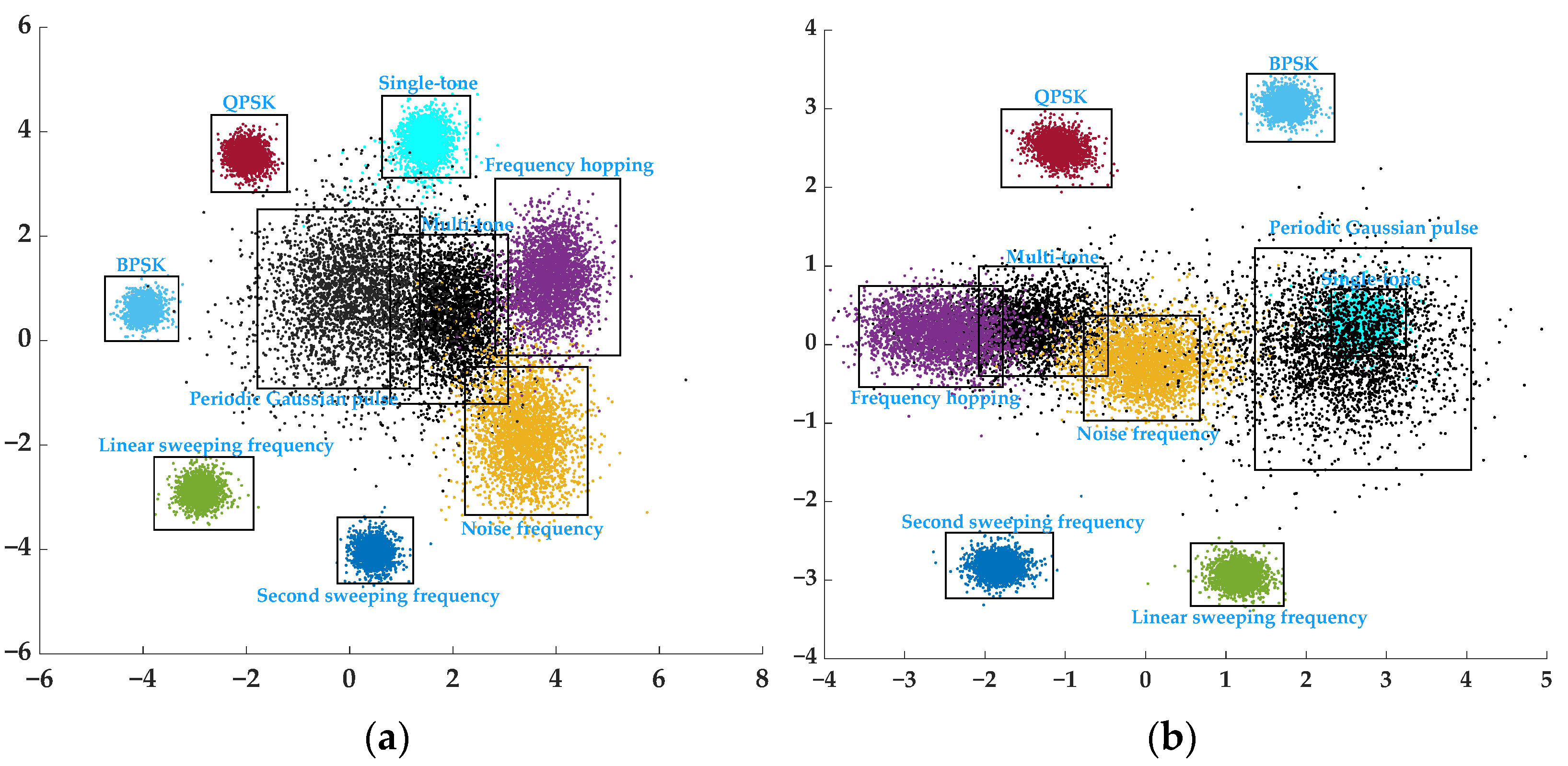
5.5. Visual Analysis of Featrue Space

In order to visually analyze the feature space of the samples, the number of neurons in the last FC layer is set to 2. Multitone jamming and periodic Gaussian pulse jamming are chosen as unknown classes and the other types as known classes. HCPL and GCPL are retrained using CNN, shown in Figure 6b, as the feature extractor, and the test signal under JNR = 0 dB is the input. Figure 11a,b is the two-dimensional distribution in the feature space using HCPL and GCPL, respectively. The black points represent unknown class signal features, while other different color points represent different known class signal features.

It can be seen from Figure 11a that the KIS features of HCPL appear in the periphery of the feature space, and they avoid a large amount of overlap between the KIS features and UIS features in the inside of the feature space. However, from Figure 11b, the KIS features of GCPL appear in the interior of the feature space, and it leads to a lot of overlap between the UIS features and KIS features; among them, the features of periodic Gaussian pulse jamming overlap those of single-tone jamming. Therefore, the OSR performance of HCPL is better than that of GCPL. It is also worth noting that the features of multitone jamming are closer to those of frequency hopping jamming than the others in GCPL and HCPL. Although, according to the principle of maximum entropy, the unknown class is more likely to embed inside of the feature space, as in periodic Gaussian pulse jamming, because there are certain similarities between frequency hopping jamming and multitone jamming; that is, there are multiple frequencies, and the network is more likely to provide a higher score to the frequency hopping jamming than to unknown multitone jamming.

6. Conclusions

We proposed the HCPL and HAFRNet for the OSR of the interference signals. The HCPL uses a hybrid loss function combining the inner product-based cross-entropy loss, center loss and prototype radius loss for training the parameters of the network. HAFRNet uses the feature reuse structure and HDAM to improve the OSR performance of the interference signals under different openness while greatly reducing the computation and storage complexity. The experiment results show that HCPL can indeed improve the unknown class rejection performance, while HAFRNet can make HCPL more stable and get better OSR performance, and the proposed method has better OSR performance than CG-Encoder under different openness and various JNR and with a lower complexity than CG-Encoder.

Our work can only distinguish the unknown class signals from the known class signals but cannot further identify each type of unknown class signal. In a future work, we will achieve open-world recognition of the interference signals by combining other techniques such as deep clustering and extend our experiments to air scenarios to evaluate the performances of the proposed method in real-world environments.

References

1. Tang, Y.; Zhao, Z.; Li, C.; Ye, X. Open Set Recognition Algorithm Based on Conditional Gaussian Encoder. Math. Biosci. Eng. 2021, 18, 6620–6637. [Google Scholar] [CrossRef] [PubMed]
2. Zhang, M.; Wang, H.; Zhou, K.; Cao, P. Low Probability of Intercept Radar Signal Recognition by Staked Autoencoder and SVM. In Proceedings of the 10th International Conference on Wireless Communications and Signal Processing (WCSP), Hangzhou, China, 18–20 October 2018; pp. 1–6. [Google Scholar]
3. Wang, G.S.; Ren, Q.H.; Jiang, Z.; Liu, Y.; Xu, B. Jamming Classification and Recognition in Transform Domain Communication System Based on Signal Feature Space. Syst. Eng. Electron. 2017, 39, 1950–1958. [Google Scholar]
4. Guoce, H.U.A.N.G.; Guisheng, W.A.N.G.; Qinghua, R.E.N.; Shufu, D.O.N.G.; Weiting, G.A.O.; Shuai, W.E.I. Adaptive Recognition Method for Unknown Interference Based on Hilbert Signal Space. J. Electron. Inf. Technol. 2019, 41, 1916–1923. [Google Scholar]
5. Gao, M.; Li, H.; Jiao, B.; Hong, Y. Simulation Research on Classification and Identification of Typical Active Jamming Against LFM Radar. In Proceedings of the 11th International Conference on Signal Processing Systems (ICSPS), Chengdu, China, 15–17 November 2019; p. 11384. [Google Scholar]
6. Lv, Q.; Qin, H. An Improved Method Based on Time-Frequency Distribution to Detect Time-Varying Interference for GNSS Receivers with Single Antenna. IEEE Access 2019, 7, 38608–38617. [Google Scholar] [CrossRef]
7. Hao, Z.; Yu, W.; Chen, W. Recognition Method of Dense False Targets Jamming Based on Time-frequency Atomic Decomposition. J. Eng. 2019, 2019, 6354–6358. [Google Scholar] [CrossRef]
8. Wang, Y.; Sun, B.; Wang, N. Recognition of Radar Active-jamming through Convolutional Neural Networks. J. Eng. 2019, 2019, 7695–7697. [Google Scholar] [CrossRef]
9. Liu, Q.; Zhang, W. Deep Learning and Recognition of Radar Jamming Based on CNN. In Proceedings of the 12th International Symposium on Computational Intelligence and Design (ISCID), Hangzhou, China, 14–15 December 2019; pp. 208–212. [Google Scholar]
10. Qu, Q.; Wei, S.; Liu, S.; Liang, J.; Shi, J. JRNet: Jamming Recognition Networks for Radar Compound Suppression Jamming Signals. IEEE Trans. Veh. Technol. 2020, 69, 15035–15045. [Google Scholar] [CrossRef]
11. Shao, G.; Chen, Y.; Wei, Y. Convolutional Neural Network-Based Radar Jamming Signal Classification with Sufficient and Limited Samples. IEEE Access 2020, 8, 80588–80598. [Google Scholar] [CrossRef]
12. Tang, Y.; Zhao, Z.; Ye, X.; Zheng, S.; Wang, L. Jamming Recognition Based on AC-VAEGAN. In Proceedings of the 15th IEEE International Conference on Signal Processing (ICSP), Beijing, China, 6–9 December 2020; pp. 312–315. [Google Scholar]
13. Wu, Q.; Sun, Z.; Zhou, X. Interference Detection and Recognition Based on Signal Reconstruction Using Recurrent Neural Network. In Proceedings of the IEEE Globecom Workshops (GC Wkshps), Hawaii Big Island, HI, USA, 9–13 December 2019; pp. 1–6. [Google Scholar]
14. Man, F.E.N.G.; Zinan, W.A.N.G. Interference Recognition Based on Singular Value Decomposition and Neural Network. J. Electron. Inf. Technol. 2020, 42, 2573–2578. [Google Scholar]
15. Peng, S.; Sun, S.; Yao, Y.D. A Survey of Modulation Classification Using Deep Learning: Signal Representation and Data Preprocessing. IEEE Trans. Neural Netw. Learn. Syst. 2021, 1–19. [Google Scholar] [CrossRef] [PubMed]
16. Wu, Y.; Sun, Z.; Yue, G. Siamese Network-based Open Set Identification of Communications Emitters with Comprehensive Features. In Proceedings of the 6th International Conference on Communication, Image and Signal Processing (CCISP), Chengdu, China, 19–21 November 2021; pp. 408–412. [Google Scholar]
17. Karunaratne, S.; Hanna, S.; Cabric, D. Open Set RF Fingerprinting using Generative Outlier Augmentation. In Proceedings of the IEEE Global Communications Conference (GLOBECOM), Madrid, Spain, 7–11 December 2021; pp. 1–7. [Google Scholar]
18. Xu, Y.; Qin, X.; Xu, X.; Chen, J. Open-Set Interference Signal Recognition Using Boundary Samples: A Hybrid Approach. In Proceedings of the International Conference on Wireless Communications and Signal Processing (WCSP), Nanjing, China, 21–23 October 2020; pp. 269–274. [Google Scholar]
19. Gong, J.; Qin, X.; Xu, X. Multi-Task Based Deep Learning Approach for Open-Set Wireless Signal Identification in ISM Band. IEEE Trans. Cogn. Commun. Netw. 2022, 8, 121–135. [Google Scholar] [CrossRef]
20. Miller, D.; Sunderhauf, N.; Milford, M.; Dayoub, F. Class Anchor Clustering: A Loss for Distance-based Open Set Recognition. In Proceedings of the IEEE Winter Conference on Applications of Computer Vision (WACV), Waikoloa, HI, USA, 3–8 January 2021; pp. 3569–3577. [Google Scholar]
21. Yang, H.M.; Zhang, X.Y.; Yin, F.; Liu, C.L. Robust Classification with Convolutional Prototype Learning. In Proceedings of the IEEE/CVF Conference on Computer Vision and Pattern Recognition, Salt Lake City, UT, USA, 18–23 June 2018; pp. 3474–3482. [Google Scholar]
22. Yang, H.M.; Zhang, X.Y.; Yin, F.; Yang, Q.; Liu, C.L. Convolutional Prototype Network for Open Set Recognition. IEEE Trans. Pattern Anal. Mach. Intell. 2020, 44, 2358–2370. [Google Scholar] [CrossRef] [PubMed]
23. Awan, M.J.; Rahim, M.S.M.; Salim, N.; Rehman, A.; Nobanee, H.; Shabir, H. Improved Deep Convolutional Neural Network to Classify Osteoarthritis from Anterior Cruciate Ligament Tear Using Magnetic Resonance Imaging. J. Pers. Med. 2021, 11, 1163. [Google Scholar] [CrossRef] [PubMed]
24. Bendale, A.; Boult, T.E. Towards Open Set Deep Networks. In Proceedings of the IEEE Conference on Computer Vision and Pattern Recognition (CVPR), Seattle, WA, USA, 27–30 June 2016; pp. 1563–1572. [Google Scholar]
25. Kardan, N.; Stanley, K.O. Mitigating Fooling with Competitive Overcomplete Output Layer Neural Networks. In Proceedings of the International Joint Conference on Neural Networks (IJCNN), Anchorage, AK, USA, 14–19 May 2017; pp. 518–525. [Google Scholar]
26. Neal, L.; Olson, M.; Fern, X.; Wong, W.K.; Li, F. Open Set Learning with Counterfactual Images. In Proceedings of the 15th European Conference on Computer Vision (ECCV), Munich, Germany, 8–14 September 2018; pp. 620–635. [Google Scholar]
27. Jo, I.; Kim, J.; Kang, H.; Kim, Y.D.; Choi, S. Open Set Recognition by Regularising Classifier with Fake Data Generated by Generative Adversarial Networks. In Proceedings of the IEEE International Conference on Acoustics, Speech and Signal Processing (ICASSP), Calgary, AB, Canada, 15–20 April 2018; pp. 2686–2690. [Google Scholar]
28. Yang, Y.; Hou, C.; Lang, Y.; Guan, D.; Huang, D.; Xu, J. Open-set Human Activity Recognition Based on Micro-Doppler Signatures. Pattern Recognit. 2019, 85, 60–69. [Google Scholar] [CrossRef]
29. Yue, Z.; Wang, T.; Sun, Q.; Hua, X.S.; Zhang, H. Counterfactual Zero-Shot and Open-Set Visual Recognition. In Proceedings of the IEEE/CVF Conference on Computer Vision and Pattern Recognition (CVPR), Nashville, TN, USA, 19–25 June 2021; pp. 15399–15409. [Google Scholar]
30. Kong, S.; Ramanan, D. OpenGAN: Open-Set Recognition via Open Data Generation. In Proceedings of the IEEE/CVF International Conference on Computer Vision, 10 March 2021; pp. 813–822. Available online: https://arxiv.org/abs/2104.02939 (accessed on 20 March 2022).
31. Hendrycks, D.; Mazeika, M.; Dietterich, T. Deep Anomaly Detection with Outlier Exposure. In Proceedings of the 7th International Conference on Learning Representations (ICLR), New Orleans, LA, USA, 6–9 May 2019. [Google Scholar]
32. Sun, X.; Yang, Z.; Zhang, C.; Ling, K.V.; Peng, G. Conditional Gaussian Distribution Learning for Open Set Recognition. In Proceedings of the IEEE/CVF Conference on Computer Vision and Pattern Recognition (CVPR), Seattle, WA, USA, 13–19 June 2020; pp. 13477–13486. [Google Scholar]
33. Wen, Y.; Zhang, K.; Li, Z.; Qiao, Y. A Discriminative Feature Learning Approach for Deep Face Recognition. In Proceedings of the 14th European Conference on Computer Vision (ECCV), Amsterdam, The Netherlands, 11–14 October 2016; pp. 499–515. [Google Scholar]
34. Geng, C.; Huang, S.J.; Chen, S. Recent Advances in Open Set Recognition: A Survey. IEEE Trans. Pattern Anal. Mach. Intell. 2021, 43, 3614–3631. [Google Scholar] [CrossRef] [PubMed] [Green Version]
35. He, K.; Zhang, X.; Ren, S.; Sun, J. Deep Residual Learning for Image Recognition. In Proceedings of the IEEE Conference on Computer Vision and Pattern Recognition (CVPR), Las Vegas, NV, USA, 27–30 June 2016; pp. 770–778. [Google Scholar]
36. Huang, G.; Liu, Z.; Van Der Maaten, L.; Weinberger, K.Q. Densely Connected Convolutional Networks. In Proceedings of the IEEE Conference on Computer Vision and Pattern Recognition (CVPR), Honolulu, HI, USA, 21–26 July 2017; pp. 2261–2269. [Google Scholar]
37. Hu, J.; Shen, L.; Sun, G. Squeeze-and-Excitation Networks. IEEE Trans. Pattern Anal. Mach. Intell. 2020, 42, 2011–2023. [Google Scholar] [CrossRef] [PubMed] [Green Version]
38. Dhamija, A.R.; Günther, M.; Boult, T. Reducing Network Agnostophobia. In Proceedings of the 32nd Conference on Neural Information Processing Systems (NIPs), Montreal, QC, Canada, 2–8 December 2018; pp. 9157–9168. [Google Scholar]
39. Chen, G.; Qiao, L.; Shi, Y.; Peng, P.; Li, J.; Huang, T.; Tian, Y. Learning Open Set Network with Discriminative Reciprocal Points. In Proceedings of the 16th European Conference on Computer Vision (ECCV), Glasgow, UK, 23–28 August 2020; pp. 507–522. [Google Scholar]
Figure 1. Convolutional prototype learning architecture.
Applsci 12 04380 g001
Figure 2. Feature reuse structure with a TAM.
Applsci 12 04380 g002
Figure 3. HDAM structure.
Applsci 12 04380 g003
Figure 4. HAFRNet.
Applsci 12 04380 g004
Figure 5. Classification and rejection process.
Applsci 12 04380 g005
Figure 6. Two feature extractors that are used in HCPL: (a) FRNet and (b) CNN.
Applsci 12 04380 g006
Figure 7. Effects of the hyperparameters in HCPL. (a) The classification accuracy under specific λ c . (b) AURoc under specific λ c . (c) The classification accuracy under specific λ r . (d) AURoc under specific λ r .
Applsci 12 04380 g007
Figure 8. OSR performance of the HCPL using different feature extractors. (a) The classification accuracy of HCPL using three feature extractors. (b) AURoc of HCPL using three feature extractors.
Applsci 12 04380 g008
Figure 9. Variance of AURoc using different feature extractors.
Applsci 12 04380 g009
Figure 10. OSR performance of different methods under different openness. (a) The classification accuracy and AURoc using dataset Jamming-3, (b) the classification accuracy and AURoc using dataset Jamming-5 (c) the classification accuracy and AURoc using dataset Jamming-7.
Applsci 12 04380 g010
Figure 11. Visualization of the 2D feature space. (a) HCPL feature space and (b) GCPL feature space.
Applsci 12 04380 g011