Article

Speed-Flow-Geometric Relationship for Urban Roads Network

by
Tareq M. Al-Bahr
1,
Sitti Asmah Hassan
1,*,
Othman Che Puan
2,
Nordiana Mashros
1 and
Nur Sabahiah Abdul Sukor
3
1
Faculty of Engineering, School of Civil Engineering, Universiti Teknologi Malaysia (UTM), Skudai 81310, Malaysia
2
Department of Civil Engineering, Engineering College, Universiti Malaysia Pahang, Lebuhraya Tun Razak, Kuantan 26300, Malaysia
3
School of Civil Engineering, Universiti Sains Malaysia, Nibong Tebal 14300, Malaysia
*
Author to whom correspondence should be addressed.
Appl. Sci. 2022, 12(9), 4231; https://doi.org/10.3390/app12094231
Submission received: 7 March 2022 / Revised: 9 April 2022 / Accepted: 15 April 2022 / Published: 22 April 2022
(This article belongs to the Section Civil Engineering)

Abstract

:
Speed on the urban roads is significantly affected by the surrounding geometric and traffic parameters. Based on this fact, we ascertained the impact of the geometric and traffic parameters on the average travel speed of the urban roads network. Herein, 197 urban road segments in Johor (Malaysia) with diverse features were randomly selected. The average travel speed and volume of the traffic on these road segments were measured using the moving observer method (MOM). Meanwhile, these roads’ features were recorded via the direct visual inspection. Various geometric (density of the traffic calming speed, right-turn driveway, access, and right-turn) and cross-sectional (median, number of lanes, and side friction) parameters were considered. First, 14 multilinear models constructed via multilinear regression analysis were developed for traffic volume scenarios (in veh/h and pcu/h). Then, 10 models were adopted to evaluate the geometric parameters’ influence on the average travel speed for the selected roads. The results revealed a considerable impact of some geometric and traffic parameters on the average travel speed for the studied urban roads. Furthermore, the density of traffic calming speed, driveway, and intersection per 1 km of urban road segment one for each parameter was found to reduce the speed of the vehicles from 1.3 to 0.22 km/h. The combination of the road cross-section features such as median, number of lanes, and side friction strongly affected the observed speed variation. It is asserted that the developed model may facilitate the Malaysian urban roads network management to provide better traffic performance with higher mobility and safer roads design and planning, thereby offering a gateway toward sustainability.

1. Introduction

The speed-flow relationship became significant for the transportation management and planning, especially for the traffic operation evaluation [1,2,3,4]. In addition, this relationship is used as an economic analyzer for transportation planning, along with road pricing system and traffic assignment [2,3,5,6,7]. Compared to the rural roads’ sides, the urban ones facilitate very high densities of people and businesses (shops). In the Highway Capacity Manual 2010, the urban roads were defined as a street having moderately higher densities of the driveway entrance, traffic signals and disrupting signs for the STOP or YIELD in every two miles separation or below [8]. Consequently, the urban roads network authority is unable to maintain the high-quality road operating services. For providing an urban road facility with satisfactory operational performance, it is necessary to evaluate and analyze the real traffic flow condition under the complex geometric and traffic parameters. Herein, the speed-flow relationship play a paramount role for designing and planning the urban roads network towards excellent performance [2,7,9].
Several studies showed that due to the enhancement of the geometric and traffic features of the urban road facility, a gradual improvement of the speed-flow model occurred [10,11,12]. In addition, some of the reports on speed-flow relationship issues related to the urban roads focused on the congestion and capacity [12,13]. The applications for these models were predetermined based on a few geometric parameters such as signal intersection [11], signal timing [14], road width [15,16,17,18,19], and spacing length between intersections [10]. Other speed-flow relationship models evaluated the impact of the geometric and traffic parameters considered as numerical coefficients [20,21,22,23]. Nevertheless, all these studies confirmed that the geometric and traffic parameters improvement can positively influence the speed-flow relationship for the urban roads network. For instance, Leong et al. [20] developed a speed-flow relationship model based on certain geometric parameters such as lane width, lateral clearance, and access point density. In addition, various other parameters such as pavement conditions, time of days, and heavy vehicles percentage on the average speed under adverse road weather conditions were considered to build a speed-flow model [22]. The inclusion of the pavement condition and heavy vehicles’ percentages in the speed-flow model was shown to impact the travel speed at maximum.
Prahara and Prasetya [21] proposed a linear model among the average speed and vehicle classes of the motorcycles, light vehicles, and heavy vehicles. The speed-flow relationship was shown to be greatly affected by the motorcycle’s percentage in the traffic stream. In addition, some other geometric and traffic parameters like number of lanes [24,25], side friction [26,27] and median [28,29] were shown to appreciably influence the travel speed on the urban roads. Despite the strong influence of these parameters on the speed for the urban roads network they are seldom considered in the speed-flow relationship model development. On top, the parameters like traffic calming speed and right-turn driveways were never addressed in the speed-flow relationship models. It is believed that the inclusion of these parameters in the proposed model can provide a better insight concerning their impact on the speed-flow relationship. In this perception, we examined the effects of various geometric and traffic parameters on the average travel speed for the urban roads network. A new multilinear model was proposed to determine the impact of these parameters on the speed for the urban roads network.

2. Related Literatures Overview

2.1. Characteristics of Speed-Flow Relationship Models

In the science and engineering of traffics flow, the concept of speed-flow relationship is essential because it includes the interaction between two significant parameters like travel speed and flow. Thus, revised updates of the speed-flow relationship became necessary depending on the composition change of the vehicles and increased demands of the traffic flow, enabling an automatic data collection in a more comprehensive way [30]. In addition, an improvement of the geometric and traffic parameters surrounding the urban roads network was shown to enhance the speed-flow relationship [12]. In this view, some relevant literatures on the speed-flow relationship models’ development and their assessment criteria are critically overviewed to determine the role of geometric and traffic parameters on speed-flow relationship enhancement for the urban roads network (Table 1).
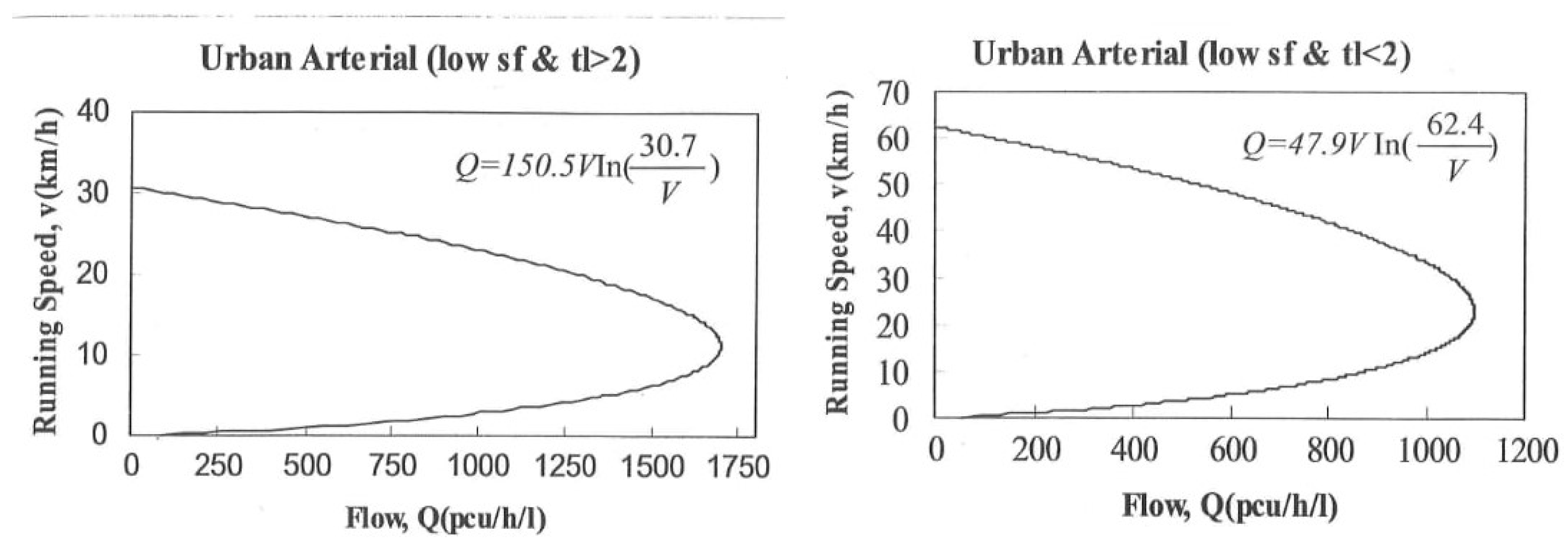
The equations of various speed-flow relationship models (Table 1) were derived mainly to determine the capacity and congestion of the urban roads inside the cities. These equations were seldom used to evaluate the speed-flow relationship based on the geometric and traffic features of the urban roads, limiting the application of each model to certain urban road features predetermined for that specific city [33]. Besides, the models dealt with parameters such as time duration at signals [14], lane width and green to cycle length time (g/c) of the signal [17], signal intersection density [31], and delay per intersection [10]. Because these models were developed for the urban road conditions, they remain unsuitable for implementation in other urban road conditions [33]. To overcome such shortcomings, the geometric and traffic parameters were included in the curves by plotting the average travel speed (ATS) and volume to capacity ratio (v/c) for four class of urban road segments as documented in the Highway Capacity Manual (HCM, 1985) [34]. Furthermore, these urban road segments were represented through other parameters like spacing between signal and free-flow speed (FFS). Later, these curves were improved in the HCM 2000 edition [5] and explained via the travel speed to v/c correlation. However, these curves were designed based on different parameters affecting the travel speed on the urban road segments such as v/c, free-flow speed (FFS), signal densities, and classes of urban roads [5]. Figure 1 shows a series of logarithm curves plotted between the average travel speed and traffic volume (Malaysian Highway Capacity Manual, MHCM) [2]. Each curve represents a predefined side friction condition of the urban road that was determined according to the number of intersections and driveways on the road segment.
Pei et al. conducted study in Hong Kong [35] and developed an exponential speed-flow-geometric model for the urban roads. It used the sensitivity parameter (α) to represent the weather conditions, geometries of the roads and control of traffic. Particularly, the model included the widths, gradients, ramps control, lanes operations, and speed limits of the roads in addition to the rainfall. The speed-flow-geometric model equation took the form:
u = u f   e x p ( α v n / n )
where u and   u f are the corresponding average travel speed and free-flow speed respectively; v is the traffic flow volume and n   is a power parameter. Although this model considered a specific range of geometric parameters for the urban roads, the impact of these parameters on the speed-flow-geometric correlation was not explicitly explained.
Ali et al. [36] proposed a speed-flow-geometric model that included a wide range of geometric and traffic parameters such as segment length, median type, and access density [36]. A multilinear regression analysis was used. The model equation yields:
ln R T M i l e = 3.7 0.05   F F S + 0.028   I n v ( S e g . L e n g t h ) + 0.03 ln ( T M o v ) + 0.1   L n ( T F l o w ) 0.02 ( M T y p e ) + 0.019 ln ( A c c D e n )
The impact of various geometric and traffic parameters of urban roads including free-flow speed ( F F S ), segment length ( S e g .   L e n g t h ), percentage of turning movement at the downstream signalized intersection ( T M o v ), median type ( M T y p e ), and access density in points per mile ( A c c D e n ) against running speed ( R T /   M i l e ) together with traffic volume ( T F l o w ) on the speed-flow-geometric relationship were examined. The results showed that the vehicles running time on the urban street can significantly be influenced (statistically) by the free-flow speed, spacing between signals, traffic flow rate, and median type.
Munawar [37] has introduced a multivariable linear equation to predict the traffic flow speed and various other traffic factors for the urban roads in Indonesia. In the equation, independent variables were a series of geometric and traffic parameters and the dependent variable was the traffic speed given by:
Y = a1 X1 + a2 X2 + a3 X3 + a4 X4 + a5 X5 + a6 X6 + a7 X7 + a8 X8 + a9 X9 + a10 X10 + k
where Y is speed (km/h), X1, X2, X3, X4, X5, X6, X7, X8, X9 and X10 are the number of non-motorized vehicles, stops of the city buses (veh/200 m/h), pedestrian movement (pedestrian/200 m/h), parked/stopped passenger car (veh/200 m/h), vehicles entered into the street (veh/200 m/h), vehicles exited from the street (veh/200 m/h), passenger cars move per hour (veh/h), heavy vehicles per hour (veh/h), motorcycles per hour (veh/h), total vehicles per hour (veh/h), respectively; a1 to a10 are the respective coefficients; k is a constant factor.
It is important to note that most of the parameters in the studied model equation were related to the traffic features rather than the geometric features for the studied urban roads. The abovementioned linear models were proposed to determine the impact of various kinds of geometric parameters (as coefficients) on the speed-flow-geometric relationship of urban roads. However, in the current work, any given parameter value observed in the field (urban roadways) can immediately be substituted in the equation without being supplied from the earlier types of speed-flow-geometric relationship models. Thus, the urban roads authority can inspect the impact of various geometric and traffic parameters on the speed-flow-geometric relationship by utilizing their numerical values.

2.2. Regression Analysis

Many studies employed the regression analysis to develop the speed-flow relationship models [7,36,37,38,39,40,41]. Empirically, this technique was widely used in traffic flow analysis such as forecasting the accident rates, congestions, and fitting the fundamental relationships between the traffic terms (speed, density, and volume) [12,40,42,43,44]. Multilinear regression analysis is a statistical method useful for examining the correlation among solitary dependent variable (called response) and several independent variables (called predictive) [45]. Among all the statistical methods, multilinear regression analysis is the most widely used one [46]. The objective of multilinear regression analysis technique is to use the values of known independent variables for predicting the distinct dependent variable’s value being selected by researchers [45]. Generally, a multilinear regression model equation for k independent can be written as:
Y = β01 X1 + β2 X2 + ……. + βk Xk + E
where β0 to βk are the unknown regression coefficients need to be determined; E is a random error of Y approximation. {Xi1, Xi2, …, Xip, Yi} for i = 1, 2, …, k are the observations (form the calibration set) required to estimate the values β parameters.

3. Methodology

3.1. Site Description

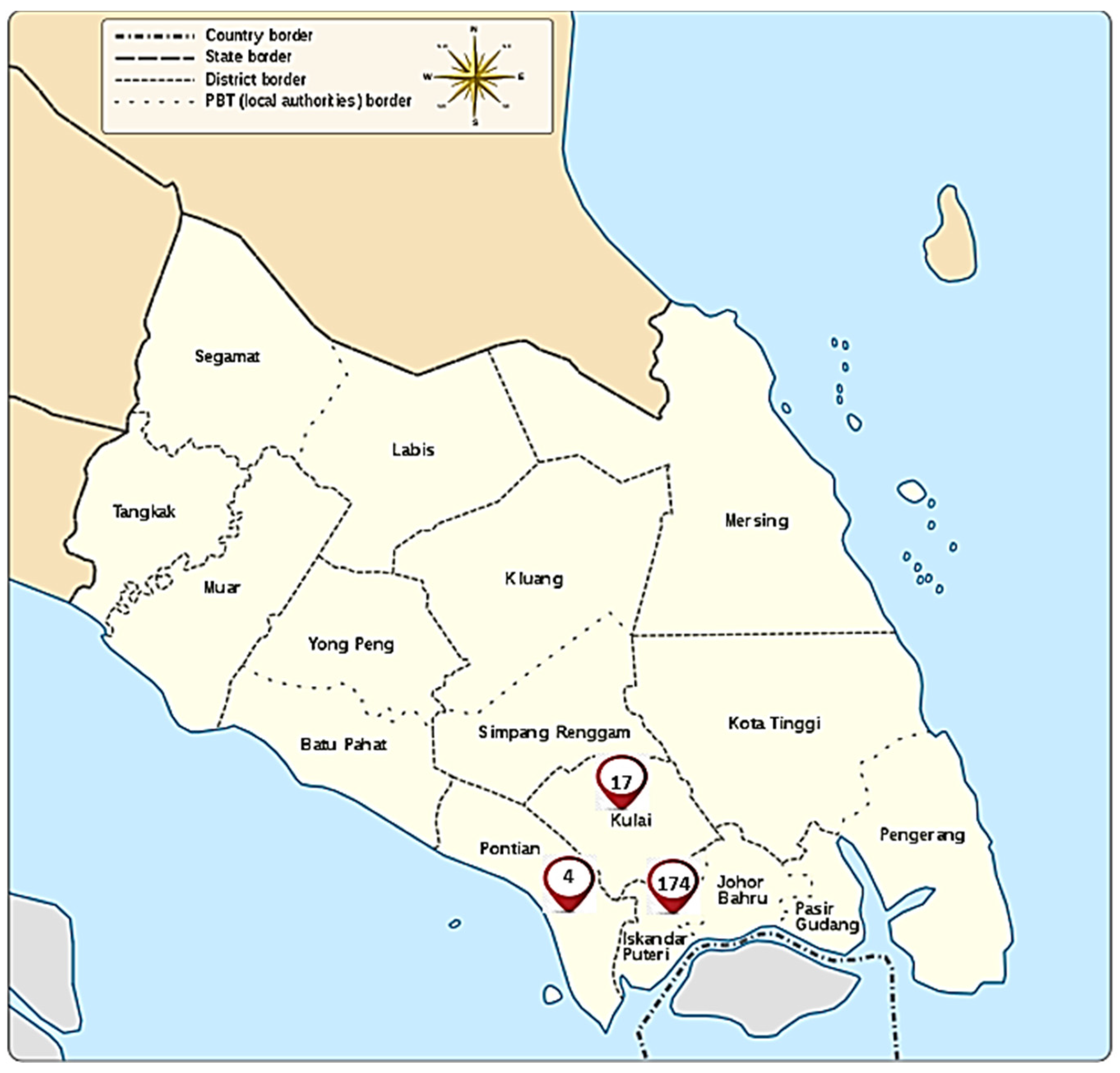
In this study, the data were collected from 197 urban roads of Johor (Malaysia) during the period May 2015 to May 2016. The traffic data from the urban roads segment was collected based on the following seven criteria: (1) they were homogeneous in terms of their geometric and traffic characteristics along the entire length; (2) they were free from any maintenance work; (3) the roads segment were two-way in nature; (4) the roads surface were in the good and prime condition during data collection; (5) the horizontal alignment of the roads segment were blunt to maintain the travel speed reasonably stable without rapid drop; (6) the urban road should not be extension to up-grade or down-grade freeway and arterial roads; (7) they were not in the residential place due to low speed (below 30 km/h). These criteria were important to avoid any disruptions in the normal traffic flow thereby influencing the driver behavior. Figure 2 shows the location of the study (Johor, Malaysia).

3.2. Data Collection

A total of 11,812 sample data were collected from the above-mentioned selected roads segment located in Johor using the moving observer method (MOM) and direct visual inspection. Being the most common method for collecting travel time data in an urban traffic environment, moving observer method (MOM) was implemented in this study [47]. In addition, this method is advantageous in measuring the times of travel and flow of traffics simultaneously [48,49,50,51,52].
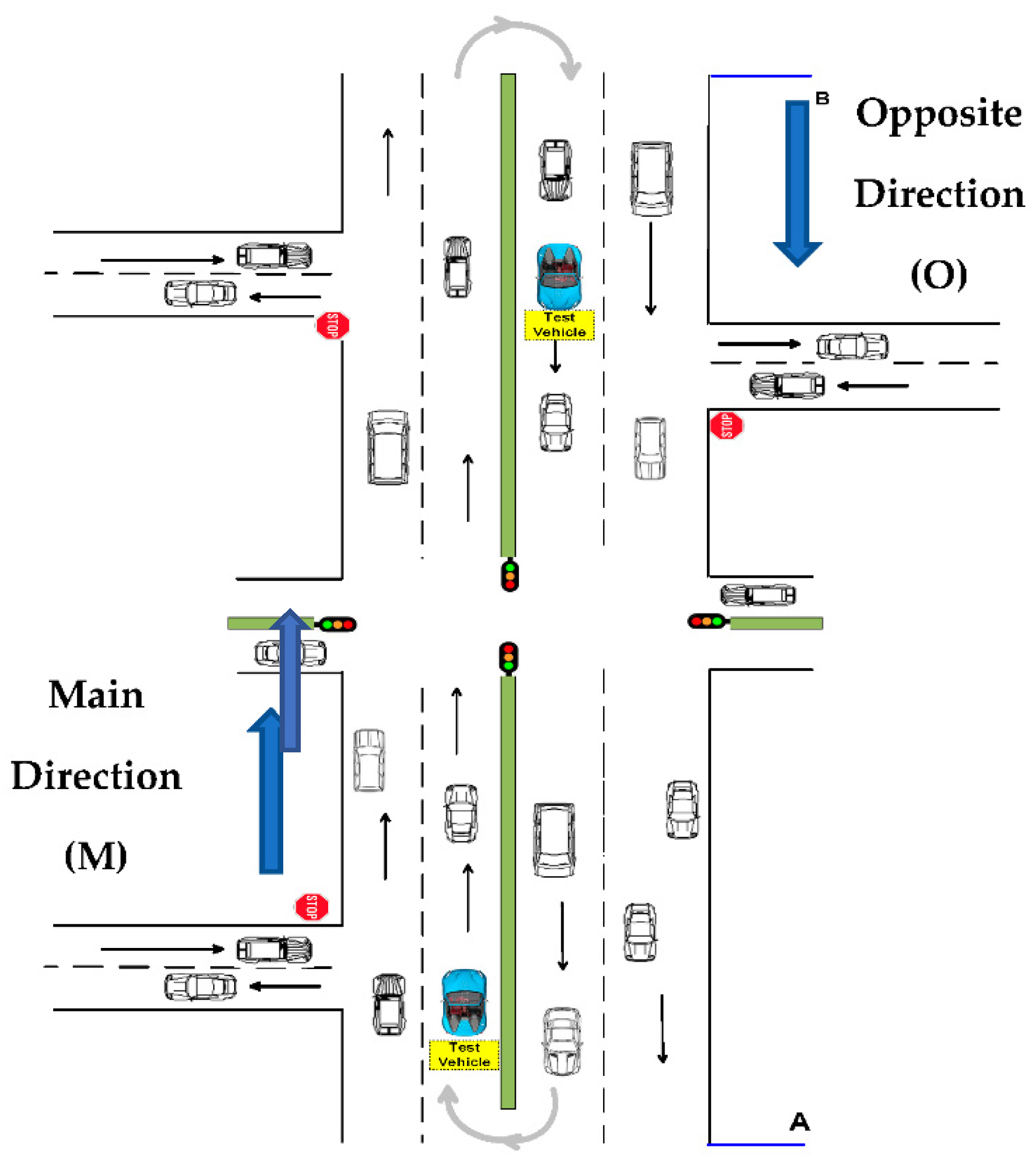
Figure 3 illustrates the schematic presentation of the moving observer method (MOM) that was applied to measure the traffic flow and travel speed in the chosen urban areas. In this method, both directions (M: main direction; O: opposite direction) of the traffic movements were considered. During the circular motion around the road segment, the travel time, number of vehicles, and distance (length of the road segment) was measured by a group of people riding the test vehicles or placing a GPS device in the test cars.
Table 2 shows the details of various traffic and geometric parameters obtained using the MOM, which were further classified as longitudinal parameters (LP) and cross-sectional parameters (CSP). The value of cross-sectional parameters (CSP) stayed at a constant value over the entire urban roads segment, whereas the value of longitudinal parameters (LP) was varied over the roads segment. These parameter classifications were useful because they defined the number of the developed models in the regression analysis.
Table 3 demonstrates the cross-sectional parameters such as median existence, side friction, and number of lanes that were used to group the surveyed urban roads useful for the model scenarios. The combination of cross-sectional parameters formed 12 groups ( 2 M × 3   N L × 2 S F = 12 ) , wherein five of them (8 to 12) were eliminated due to their insignificantly low number of the surveyed urban roads. Therefore, only seven cross-sectional parameters groups (1 to 7) were left for further analyses of the 7 regression models developed to ascertain the relationship amid average travel speed (ATS) and traffic volume (TV), traffic calming speed density (TCSD), intersection density (IntersD), access driveway density (AccessD), and right-turn driveway density (RTD) (Table 2 and Table 3). These models were constructed for two traffic volume scenarios (like veh/h and pcu/h), yielding 14 regression models. To transform veh/h to pcu/h, the conversion factors (0.22 for motorcycles, 2.27 for trucks, 1.19 for lorry, and 2.08 for bus) adopted from the MHCM (2011) [51] were used.

3.3. Model Development Using Multilinear Regression Analysis (MRA)

As aforementioned, the speed-flow-geometric relationship models between the independent variable (ATS) and dependent variables (TV, TCSD, AccessD, IntersD, and RTD) for seven surveyed urban road groups were developed using the multilinear regression analysis. Four multilinear regression analysis steps were used to select the final model. First, multilinear regression analysis dealt with the model estimation where all possible independent variables were included in the regression analysis to develop the first estimation model. Herein, all independent variables were evaluated and tabulated. In the first model estimation, the statistical regression results included the F-test, R2, t-test, and standard errors. The significant models were estimated using the F-test value [45,53,54]. When the p-value of the F-test was below 0.05 (the confidence level is 95% for the entire model development), it was declared as statistically significant. Second, multilinear regression analysis involved the model elimination wherein the backward elimination was performed for all independent variables listed in the previous step. This elimination was carried out using the t-test of each variable wherein any variable with p-value above or equal to 0.05 (≥0.05) for the t-test was removed from the regression. This process was repeated until all the independent variables confirmed that they have a significant impact on average travel speed (ATS) based on their t-test (p-value < 0.05). Third, multilinear regression analysis entailed with the model verification wherein the assumption rules for the residuals of the regression as well as the multi-collinearity condition between the independent variables was applied. In this step, the residual satisfied the assumptions test, such as linearity, homoscedasticity and independence. Furthermore, the model verified the multicollinearity value between the independent variables using the VIF index. Some literature reports revealed that VIF must be below 10 (between any two independent variables) [45,54,55]. Fourth, multilinear regression analysis dealt with the model validation that was conducted by comparing the calculated average travel speed (ATS) from the developed models with the estimated average travel speed (ATS) from the moving observer method (MOM) for the new selected urban roads segment. This comparative evaluation was performed using the t-paired test between the mean values of each average travel speed (ATS) group.

4. Results

4.1. Measured Parameter Descriptive Outcomes

Table 4 summarizes the descriptive statistical outcomes of all parameters evaluated over the surveyed urban roads.
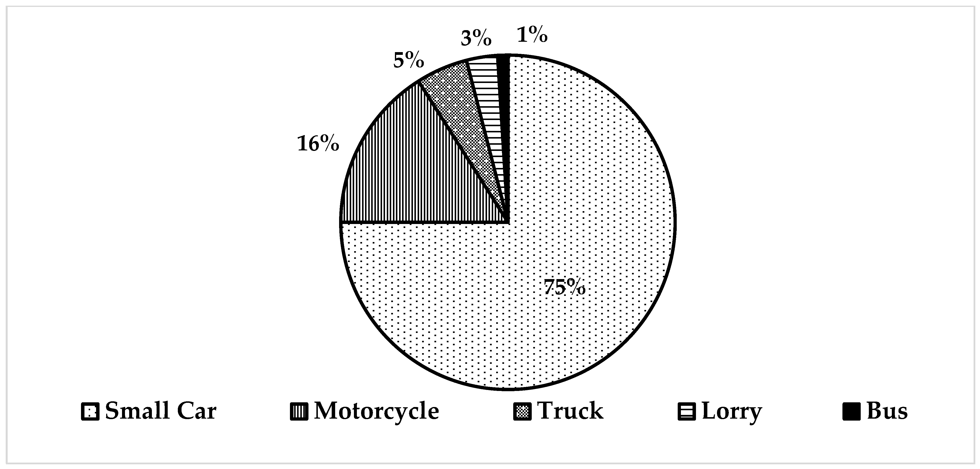
Figure 4 illustrates the percentage quantity of cross-section parameters values over the surveyed urban roads for median existence (M), number of lanes (NL), and side friction condition (SF). Figure 5 depicts the traffic volume composition over the surveyed urban roads.
The median existence in the urban roads was observed to be almost equal for both with and without median situations (Figure 4a). Most of the studied Johor roads network consisted of 2-lane roads of 58% followed by 1-lane roads of 30% and 3-lane roads of 12% (Figure 4b). In addition, the selected urban roads consisted of 56% of low side friction and 44% of high side friction condition (Figure 4c). In fact, three quarter of the traffic composition was small car (75%) whereas all the remaining four classes have the last fourth quarter of the pie chart (Figure 5).

4.2. Developed Models Features

As mentioned earlier, 14 regression models for the traffic volume (TV) scenarios in veh/h and pcu/h were developed and summarized in Table 5. Four models were found to be insignificant based on their p-value above 0.05, representing the surveyed urban roads groups with cross-section parameters features without median, 2-lanes and low side friction [M0, NL2, SF0]; and 1 median, 3-lanes and low side friction [M1, NL3, SF0]. Consequently, 10 succeed models represented the surveyed urban roads groups for cross-section parameters features [M0, NL1, SF0], [M0, NL1, SF1], [M0, NL2, SF1], [M1, NL2, SF0], and [M1, NL2, SF1] for both traffic volume in veh/h and pcu/h. All the final model equations for the cross-section parameters groups were explicitly written for the first time. Clearly, all these models showed reasonable coefficient of determination (R2) values that varied in the range of 0.62 to 0.97. In addition, the significant p-values obtained from the F-test were below 0.05 with small standard errors in the range of 0.64 to 3.37.
In the evaluation of speed-flow models we considered some additional geometric features of the road other than number of driveways and intersection density like traffic calming speed density (TCSD), right-turn driveway (RTD), number of lanes (NL), median (M), and side friction (SF). The empirical multilinear models were developed using direct values of wide range of geometric and traffic features as observed in the field. The geometric parameters included in the developed models were explicitly described as numerical coefficients. Hence, the proposed models can easily be implemented for the practical purposes depending on any empirical values. The impact of these parameters on the average travel speed (ATS) was evaluated as the values of numerical coefficients in the equations of the models. The successful models provided a correlation between average travel speed (ATS) and three geometric parameters such as traffic calming speed density (TCSD), access driveway density (AccessD) and intersection density (IntersD). The right-turn driveway density (RTD) was found to have no impact on the average travel speed (ATS). In the proposed model, the unification of the cross-section parameters was discerned to influence each coefficient of the longitudinal parameters (AccessD, TCSD, and IntersD) and average travel speed (ATS).
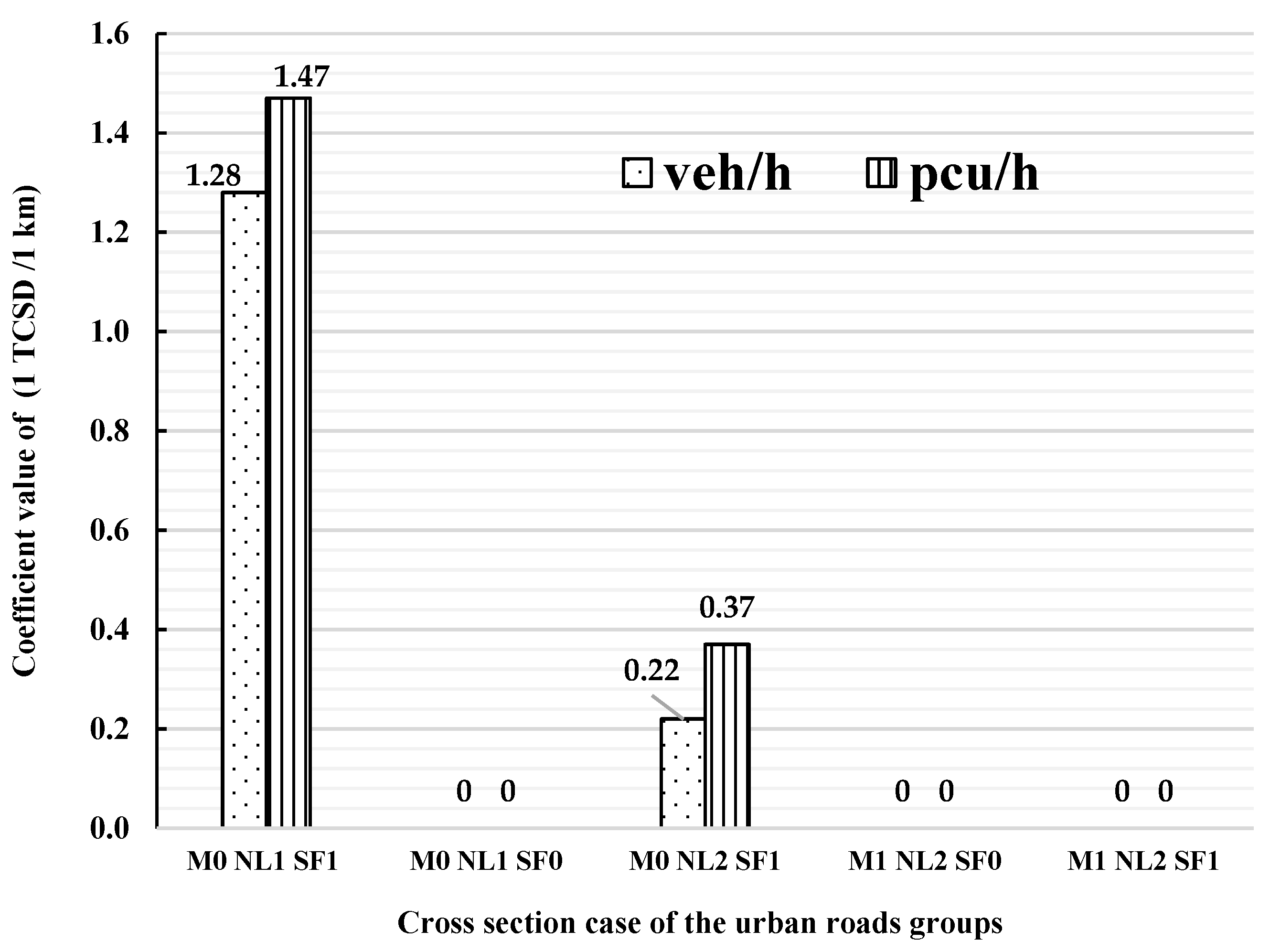
Figure 6, Figure 7 and Figure 8 display the variation of traffic calming speed density (TCSD), access driveway density (AccessD) and intersection density (IntersD) in the five successful models. The same density of 1 TCSD/km had no impact on the reduction of average travel speed (ATS) for the urban roads having the cross-section combination of no median, one lane, and low side friction [M0, NL1, SF0]; with median, two lanes, low side friction [M1, NL2, SF0]; and also with median, two lanes, and high side friction [M1, NL2, SF1]. Conversely, the same density of 1 TCSD/km could reduce the average travel speed (ATS) on the traffic flow by small amount 0.22 km/h, if the urban road had no median, two lanes, and a high side friction [M0, NL2, SF1]. Figure 6 illustrates the impact of traffic calming speed density (TCSD) on the average travel speed (ATS) for various combinations of cross-sectional features in the model for the studied urban roads segment.
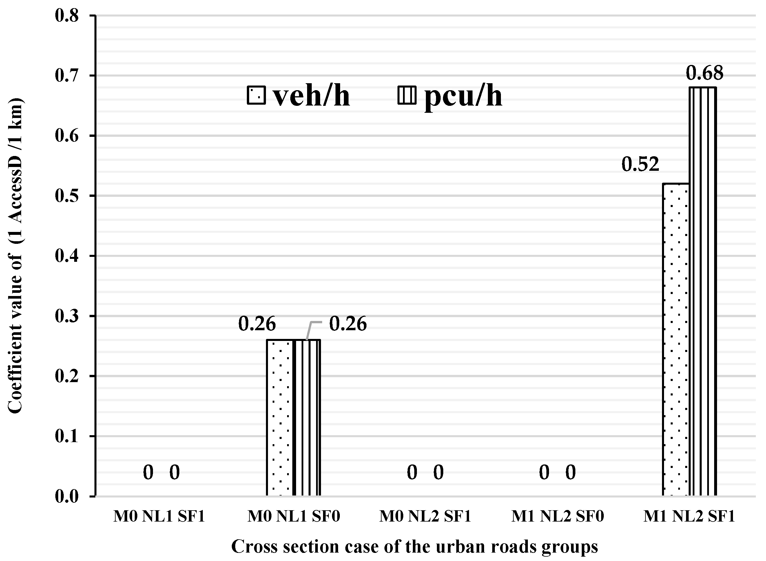
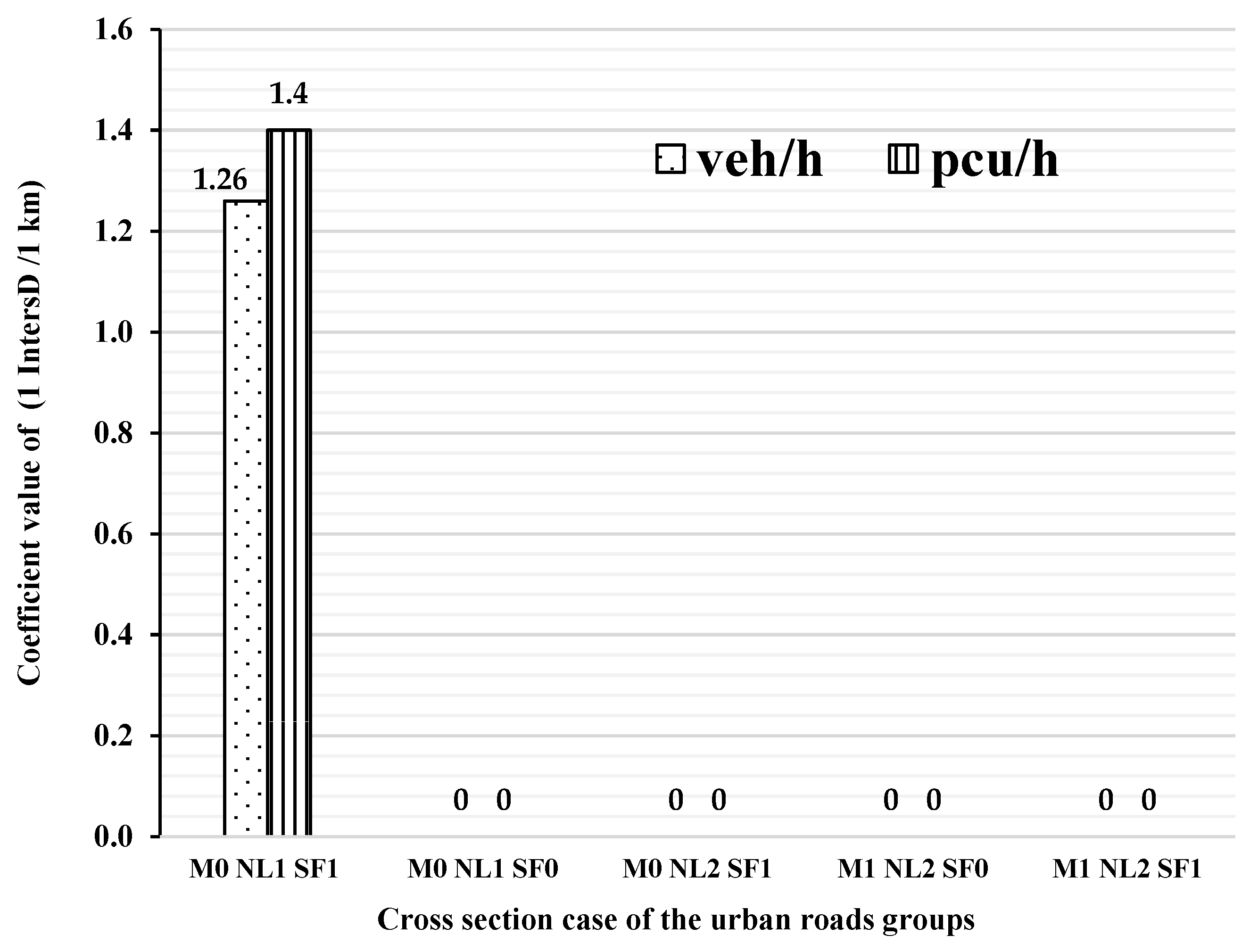
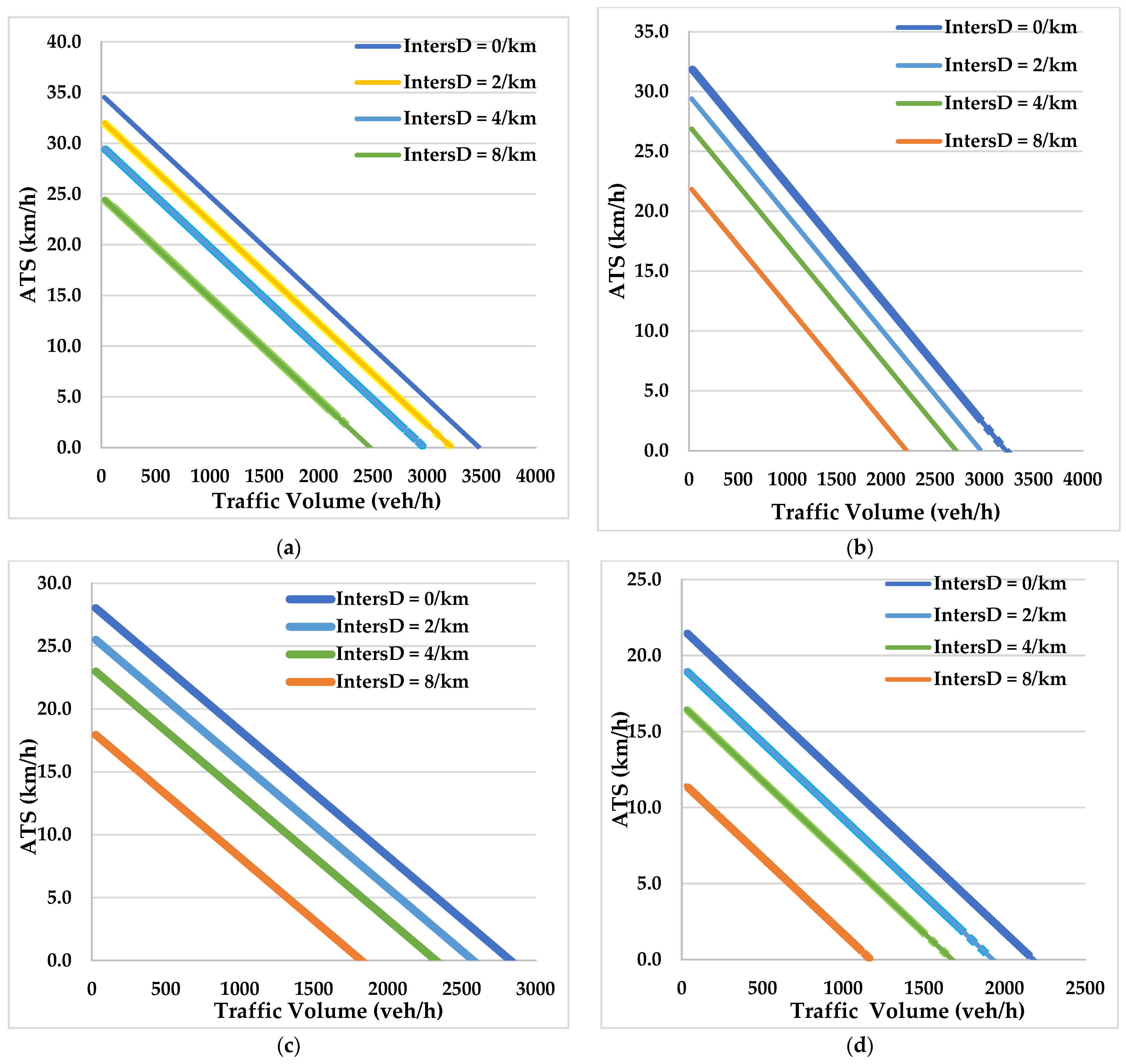
The values of average travel speed (ATS) for the urban road category [M1, NL2, SF0] remained unaffected by the variation of three geometric parameters namely traffic calming speed density (TCSD), access driveway density (AccessD) and intersection density (IntersD) (Figure 6, Figure 7 and Figure 8). However, the values of average travel speed (ATS) for the urban road category [M0, NL1, SF1] was appreciably impacted due to the variation of traffic calming speed density (TCSD) and intersection density (IntersD). Furthermore, for every 1 TCSD/km and 1 IntersD/km, the average travel speed (ATS) was reduced by 1.28 km/h and 1.26 km/h, respectively for the traffic volume in veh/h. Under the heterogeneous traffic (pcu/h) condition for every 1 TCSD/km and 1 IntersD/km, the average travel speed (ATS) value was decreased by 1.47 km/h and 1.4 km/h, respectively. On top, the access driveway density (AccessD) parameter has the highest impact on the average travel speed (ATS) value variation for the urban road category [M1, NL2, SF1].

4.3. Model Validation

Two groups of traffic volume (veh/h for Model A and pcu/h for Model B) were used in the model development. The estimated average travel speed (ATS) was compared for three cases including the observed onsite average travel speed (ATS) using the moving observer method (MOM), estimated average travel speed (ATS) in Model A and estimated average travel speed (ATS) in Model B. Statistical analysis using paired t-test was performed to evaluate any significance difference among the samples means between these three cases. Table 6 shows the results of paired t-test. The detail result of paired t-test is shown in Appendix A.
The result in Table 6 clearly shows the complete absence of any significant difference between Group 1 and Group 2 for three surveyed urban roads groups such as [M0, NL1, SF0], [M0, NL1, SF1], and [M1, NL2, SF0]. Therefore, paired t-test was conducted between estimated average travel speed (ATS) using Model A and B. Among these three surveyed urban roads groups, the [M0, NL1, SF0] and [M1, NL2, SF0] group displayed some significant differences between the average travel speed (ATS) values estimated using Model A and B. In addition, Model B that considered heterogeneous traffic volume revealed better results, indicating the stronger impacts of the urban roads segment geometric and traffic features on the average travel speed (ATS) for the studied two surveyed urban roads groups. However, for the surveyed urban roads group [M0, NL1, SF1], the paired t-test between the estimated average travel speed (ATS) using Model A and Model B in Group 3 showed no significant difference, thus adopting Model A for these surveyed urban roads group. For the surveyed urban roads group [M0, NL2, SF1] and [M1, NL 2, SF1], only Group 1 disclosed insignificant variation between the measured the average travel speed (ATS) using moving observer method (MOM) and the estimated average travel speed (ATS) using Model A, whereas Group 2 indicated a substantial difference for these two values, thus adopting Model A for these two surveyed urban roads groups.

4.4. Models Application

The final speed-flow-geometric model from Table 6 was used for predicting the average travel speed (ATS) values on the Johor roads segment. Each surveyed urban road group model enclosed a set of independent variables (longitudinal parameters, LP) with estimated free-flow speed (FFS), and range of traffic volume (TV) as shown in Table 7. A pre-specified range of values was used for the longitudinal parameters (LP) for each surveyed urban road groups of the urban roads segment.
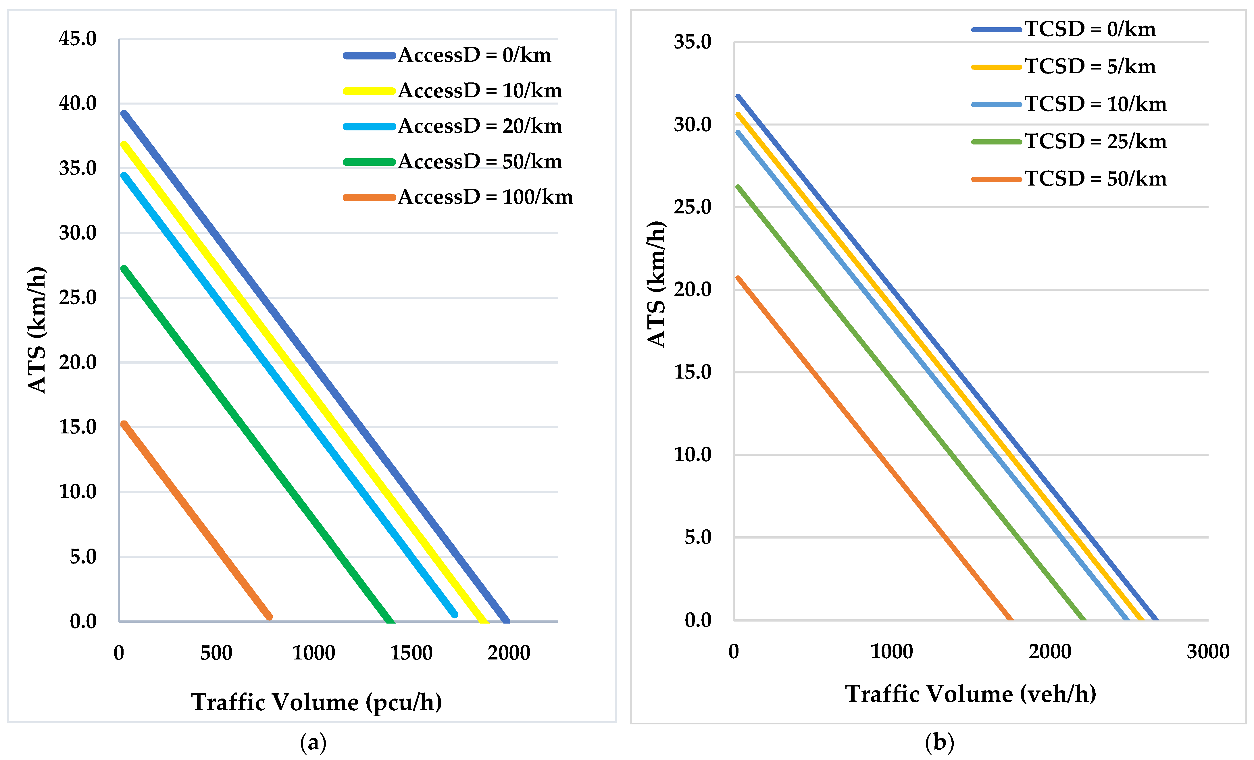
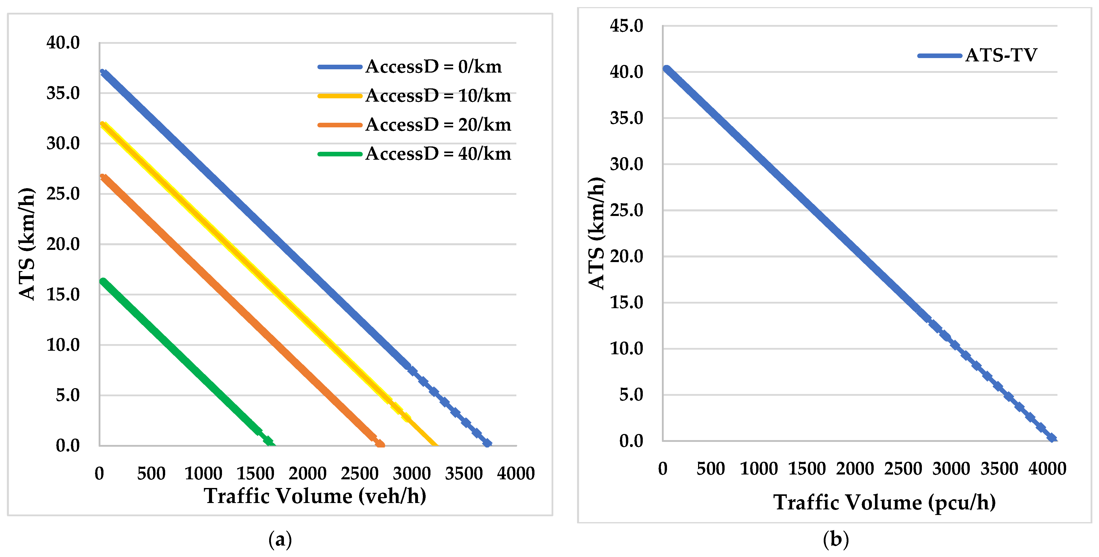
A series of linear trend lines for each value of the longitudinal parameters (LPs) were used to illustrate the variation of the average travel speed (ATS) against the traffic volume (Figure 9, Figure 10 and Figure 11). These lines were obtained by substituting the measured values of traffic calming speed density (TCSD), intersection density (IntersD), and access driveway density (AccesD) parameters into the developed speed-flow-geometric relationship equations for the five categories of cross-sectional parameters (median, number of lanes, and side friction conditions). These longitude parameters were assumed to have values within a certain range between two extremities. The highest value did not exceed the intercept value of the developed equation. This was due to the fact that only the intercept value in the equation had positive sign whereas all other longitudinal parameters in addition to the traffic volume (TV) had negative signs. Consequently, if they were bigger than the intercept, the estimated average travel speed (ATS) became zero (or negative), indicating that this speed-flow-geometric relationship equation is inapplicable. Parallel to the definition of the highest applicable value of the longitudinal parameter in the equation, a line of the speed-flow relationship could be drawn if we solve the equation for average travel speed (ATS) and traffic volume (TV) (in the case where the traffic volume is zero and the average travel speed is zero). Next, for each model, a sensible decrease in the greatest value of the longitudinal parameter, this incline line of speed-flow relationship might be traced many times downward. When the inclined speed-flow relationship line provided an irrationally small value of average travel speed (ATS), this iteration ended. In short, for each of the five urban road’s category, distinct series inclined lines of speed-flow relationship were developed.
It is obvious that the application of the speed-flow models was limited by the free-flow speed (FFS). In the proposed model, the free-flow speed (FFS) was defined as the intercept value of each succeed developed model (Table 5). The predicted average travel speed (ATS) used a particular model or equation without exceeding or equal to the free-flow speed (FFS) for any condition. In other words, if the value of the longitudinal parameter or the summation of the longitudinal parameter’s value and traffic volume was greater than the predefined value of the free-flow speed (FFS) (intercept), the model was not accepted for application because the average travel speed (ATS) values were negative.
The proposed models can fundamentally contribute in terms of the applicability in real situation wherein a broad range of geometric and traffic parameters variability in the urban road network can physically be incorporated. Therefore, the models can effectively be used as significant tools to measure the average travel speed (ATS) with diverse geometric and traffic features on the urban roads. A series of steps must be followed to achieve these goals. First, the cross-section features of the urban roads must be identified that can be determined by three parameters like the median existence, number of lanes, and condition of side friction. Consequently, it can be measured as two different integer values such as 1 = having a median, 0 = without a median, 1 = high-side friction, 0 = low-side friction, and the number of lanes (1, 2, and 3). Second, following the unification of these three cross-section features the proposed model one must select all other five models (Table 5). Third, the values of the longitude features of the urban roads must be quantified accurately that requires the density values of the facilities i.e., their numbers over the entire urban road length. Essentially, any combination of the density for the traffic calming speeds, access driveways, and intersections can be substituted in the proposed model. Fourth, the traffic volume information must be inserted in the proposed model for accurate prediction. Finally, the impact of the traffic composition in the respective models must be considered by applying the pcu conversion factor to the traffic volume.

5. Discussion

The majority of the previous models of the speed-flow-geometric relationship used few geometric parameters and suffered from various limitations. To surmount these problems, we used a wide range of geometric and traffic features and studied their impacts on the speed-flow-geometric relationship models using a multilinear regression analysis. This allowed us to identify the combined influence of median, the number of lanes, side friction condition, driveways density, intersection density, traffic calming speed device density, and right-turn driveway density on the main relationship between traffic speed and traffic volume on urban roads.
The paired t-test showed that road which has no median with one lane, regardless of the condition of side friction, requiring the conversion of traffic volume into pcu/h before the use of the developed models. The remaining three categories, namely no median, two lanes, and high side friction; with median, two lanes, and high side friction; and no median, one number of lanes, and high side friction did not provide significant difference when they converted the traffic volume from veh/h to pcu/h. Thus, these three models could be applied using traffic volume as a veh/h only.
According to the various circumstances of cross-sectional features—namely median, number of lanes, and side friction condition—a series of trend lines represented the results of the developed speed-flow relationship. All these figures of plotted lines offered as the tools for the application of the developed models in the field by the authority of urban roads. In general, the developed speed-flow-geometric relationship models can be applied for five road’s categories of cross-sectional parameters (median, number of lanes, and side friction condition). In practice, the developed model for each road’s category can be applied to any urban road that corresponds to this cross-section category, regardless of the types of longitude parameters contained in this segment. Alternately, any developed model for each category can be used broadly regardless of the type, density of any longitudinal parameter (LP) on this urban road segment, unless certain constraints for a specific parameter limits the application of this model. In detail, if an urban road without median has only one lane and low side friction, the speed-flow-geometric relationship model of this category can be applied for any kind of longitudinal parameter (LP) values except if the access driveways exceed 100 per 1 km. This value reduced to 40 the access driveway per 1 km if the urban road comes with a median and high side friction.
Regarding the traffic calming speed device (TCSD), it is applicable for all five of the road’s categories with two constraints. These two constraints are the maximum number of traffic calming speed devices (TCSD) for the developed models for the urban road segment without median and the high side friction conditions are 10/km and 50/km, respectively, for one and two lanes. Except for the instance of an urban road with no median, one lane, and high side friction, all of the model’s equations may be applied to any degree of density for the longitude parameter (LP) of intersection density. For the urban road with no median, one lane and high side friction, the speed-flow-geometric relationship may be limited to eight intersection density per km. Otherwise, all these previous certain restrictions of longitude parameters (LP)-values, the developed speed-flow-geometric relationship models of this study could be used by the urban road’s authority as a significant design and planning tool.
The average travel speed (ATS) values of the vehicles on 1 km of the urban roads was reduced considerably with the increase of density as one per 1 km in traffic calming speed devices, access driveway, and intersection by 1.28 km/h, 0.52 km/h, and 1.26 km/h respectively. This reduction of the average travel speed (ATS) relied on the various combination of median, number of lanes, and side friction conditions. For instance, for no median, one lane, and high side friction situation, the reduction of average travel speed (ATS) due to traffic calming speed device was 1.28 km/h. While the same density of traffic calming speed device with the identical cross-section features (except the number of lanes = 2) could reduce the average travel speed (ATS) value by 0.22 km/h for the urban road. However, for any other cross-sectional characteristics, the traffic calming speed device did not reduce the average travel speed (ATS). Similarly, for the density of access driveway, the average travel speed (ATS) was reduced by 0.52 km/h, and 0.26 km/h on the two cases with median, two lanes, and high side friction and no median, one lane, low side of friction, respectively. However, there was no decrease in average travel speed (ATS) for any other cases of the cross-sectional features. Due to the density of the intersection, the average travel speed (ATS) value was decreased by 1.26 km/h only for one case (no median, one lane, and high side friction). Due to the density of the right-turn driveway, the regression analysis showed no reduction in average travel speed (ATS) for all cases.
The developed models affirmed that the impact of geometric and traffic parameters on the speed-flow relationship has a wide range of variability. Particularly, the significant impact of longitude parameters on the speed-flow relationship was established to rely on a coefficient value in the model equation (Table 5 and Figure 6, Figure 7 and Figure 8). For instance, the urban road without median, one lane, and low side friction displayed the coefficient of access driveway density of 0.26. This clearly indicated that when the urban road has an access density (AccessD) value of one per 1 km, the travel speed can reduce by a factor of 0.26 times. Conversely, for the same access density (AccessD) condition and urban road with a median, two lanes, and a high side-friction condition, the travel speed can reduce by a factor of 0.52.
Based on the results, it is claimed that the multilinear equation of the proposed speed-flow-geometric relationship models can help the urban roads authority to estimate exactly the numerical quantity of average travel speed (ATS) depending on any numerical quantity of geometric variable in the field. Furthermore, this kind of model may allow the engineers and planners to predetermine the range value of speed and flow in an urban road segment based on certain exact values of surrounding geometric and traffic features. Despite the number of models developed in this study being limited for the available cross-section parameter (CSP) conditions of the urban roads segment in the Johor roads network, these models confirmed the benefits for developing the multilinear models on other urban roads network to fulfill these unavailable cross-section parameters (CSP).

6. Conclusions

We determined the impact of various geometric and traffic parameters on the speed-flow-geometric relationship for Johor (Malaysia) roads segment for the first time. The multilinear regression analysis was used to develop speed-flow-geometric relationship models with the average travel speed (ATS) as a dependent variable and diverse geometric and traffic parameters as independent variables (traffic volume (veh/h and pcu/h), traffic calming speed density, access driveway density, right-turn density, and intersection density). In addition, various cross-sectional parameters (median, number of lanes and side friction) were considered. The impact of heterogeneous vehicles composition on speed-flow-geometric relationship was evaluated. The choice of average travel speed (ATS) enabled us to measure the vehicles run and delay time over the urban roads segment. The results obtained from the proposed models confirmed the impact of these new geometric and traffic parameters on the speed-flow-geometric relationship. Parameters such as traffic calming speed devices, access driveways, and intersection density displayed a significant impact on the developed speed-flow-geometric relationship models. In addition, the factors including the side-friction conditions, access driveways, medians, and traffic calming devices has influence on the urban road mobility and safety. The variability on the numerical values of longitude parameters over the five developed models showed that the speed-flow-geometric relationship was appreciably influenced by these parameters. The present study provided a fundamental insight into the better urban mobility design for the traffic management and operation based on the many combinations of the geometric and traffic parameters. The developed speed-flow-geometric relationship models can offer a gateway to highlight future directions for urban road safety in Malaysia. It is established that the proposed model can help the authority of the urban roads network providing better urban roads with high mobility, safe design and planning, leading to sustainable development.

Author Contributions

Conceptualization, T.M.A.-B. and S.A.H.; methodology, T.M.A.-B., S.A.H. and O.C.P.; software, T.M.A.-B.; formal analysis, T.M.A.-B.; resources, S.A.H.; data curation, T.M.A.-B.; writing—original draft preparation, T.M.A.-B.; writing—review and editing, S.A.H., T.M.A.-B. and N.M.; visualization, S.A.H. and T.M.A.-B.; supervision, S.A.H. and O.C.P.; project administration, S.A.H.; funding acquisition, S.A.H. and N.S.A.S. All authors have read and agreed to the published version of the manuscript.

Funding

This research was funded by the Universiti Teknologi Malaysia, vote number Q.J130000.3651.03M34 (PY/2021/00644).

Institutional Review Board Statement

Not applicable.

Informed Consent Statement

Not applicable.

Data Availability Statement

Not applicable.

Conflicts of Interest

The authors declare no conflict of interest.

Appendix A

Detail results of validation stage for five cross-sectional cases listed in Table 6.
Table A1. Results of paired t-test for model of cross-sectional case of [M0, NL1, SF0].
Comparative
ATS Results
Paired DifferencestdfSig.
(2-Tailed)
MeanStd. DeviationStd. Error Mean95% Confidence Interval of the Difference
LowerUpper
Observed ATS from MOM Versus Predicted ATS from Category A Model (km/h) with TV in veh/h−0.4501.900.425−1.340.441−1.05190.304
Observed ATS from MOM Versus Predicted ATS from Category B Model (km/h) with TV in pcu/h−0.7501.710.383−1.550.051−1.958190.065
Predicted ATS from Categories A and B Models (km/h)0.3000.57120.1270.03260.56732.349190.030
Table A2. Results of paired t-test for model of cross-sectional case of [M0, NL1, SF1].
Comparative ATS ResultsPaired DifferencestdfSig.
(2-Tailed)
MeanStd. DeviationStd. Error Mean95% Confidence Interval of the Difference
LowerUpper
Observed ATS from MOM Versus Predicted ATS from Category A Model (km/h) with TV in veh/h−0.3363.110.803−2.061.38−0.418140.682
Observed ATS from MOM Versus Predicted ATS from Category B Model (km/h) with TV in pcu/h0.7033.2160.830−1.0782.4850.847140.411
Predicted ATS from Categories A and B Models (km/h)0.3671.0490.271−0.2140.9491.356140.197
Table A3. Results of paired t-test for model of cross-sectional case of [M0, NL2, SF1].
Comparative ATS ResultsPaired DifferencestdfSig.
(2-Tailed)
MeanStd. DeviationStd. Error Mean95% Confidence Interval of the Difference
LowerUpper
Observed ATS from MOM Versus Predicted ATS from Category A Model (km/h) with TV in veh/h−0.2571.7650.489−1.3230.809−0.525120.609
Observed ATS from MOM Versus Predicted ATS from Category B Model (km/h) with TV in pcu/h−1.2571.9320.536−2.425−0.089−2.345120.037
Predicted ATS from Categories A and B Models (km/h)−1.0000.4080.113−1.247−0.753−8.832120.000
Table A4. Results of paired t-test for model of cross-section case of [M1, NL2, SF0].
Comparative ATS ResultsPaired DifferencestdfSig.
(2-Tailed)
MeanStd. DeviationStd. Error Mean95% Confidence Interval of the Difference
LowerUpper
Observed ATS from MOM Versus Predicted ATS from Category A Model (km/h) with TV in veh/h−2.809.3632.961−9.5033.893−0.9490.368
Observed ATS from MOM Versus Predicted ATS from Category B Model (km/h) with TV in pcu/h3.2299.4502.988−3.5319.9891.08190.308
Predicted ATS from Categories A and B Models (km/h)0.4240.3390.1070.1810.6673.95190.003
Table A5. Results of paired t-test for model of cross-sectional case of [M1, NL2, SF1].
Comparative ATS ResultsPaired DifferencestdfSig.
(2-Tailed)
MeanStd. DeviationStd. Error Mean95% Confidence Interval of the Difference
LowerUpper
Observed ATS from MOM Versus Predicted ATS from Category A Model (km/h) with TV in veh/h0.1670.5770.167−0.2000.5331.00110.339
Observed ATS from MOM Versus Predicted ATS from Category B Model (km/h) with TV in pcu/h0.6670.6510.1880.2531.0813.546110.005
Predicted ATS from Categories A and B Models (km/h)0.5000.5220.1510.1680.8323.317110.007

References

  1. Cohen, S.; Zhang, M.Y. New Speed Flow Relationships for Road Network Planning in the Paris Region. In Traffic and Transportation Studies; American Society of Civil Engineers: Reston, VA, USA, 2002; pp. 389–396. [Google Scholar]
  2. Highway Planning Unit (HPU). Malaysian Highway Capacity Manual; Ministry of Works: Kuala Lumpur, Malaysia, 2006.
  3. Li, M.Z.F. A Generic Characterization of Equilibrium Speed-Flow Curves. Transp. Sci. 2008, 42, 220–235. [Google Scholar] [CrossRef]
  4. Chiguma, M.L. Analysis of Side Friction Impacts on Urban Road Links; Case Study, Dar-es-Salaam. Ph.D. Thesis, Royal Institute of Technology (KTH), Stockholm, Sweden, 2007. [Google Scholar]
  5. Transportation Research Board (TRB). Highway Capacity Manual; National Research Council: Washington, DC, USA, 2000. [Google Scholar]
  6. Li, M.Z.F. The role of speed–flow relationship in congestion pricing implementation with an application to Singapore. Transp. Res. Part B Methodol. 2002, 36, 731–754. [Google Scholar] [CrossRef]
  7. Hooper, E.; Chapman, L.; Quinn, A. The impact of precipitation on speed–flow relationships along a UK motorway corridor. Theor. Appl. Climatol. 2014, 117, 303–316. [Google Scholar] [CrossRef]
  8. Transportation Research Board (TRB). Highway Capacity Manual; National Research Council: Washington, DC, USA, 2010. [Google Scholar]
  9. Van Aerde, M.; Rakha, H. Multivariate calibration of single regime speed-flow-density relationships. In Pacific Rim TransTech Conference. 1995 Vehicle Navigation and Information Systems Conference Proceedings. 6th International VNIS. A Ride into the Future; IEEE: Piscataway, NJ, USA, 1995; pp. 334–341. [Google Scholar]
  10. Lum, K.M.; Fan, H.S.; Lam, S.H.; Olszewski, P. Speed-flow modeling of arterial roads in Singapore. J. Transp. Eng. 1998, 124, 213–222. [Google Scholar] [CrossRef]
  11. Chen, Y. Model of Traffic Speed-Flow Relationship at Signal Intersections. Open J. Appl. Sci. 2017, 7, 319–327. [Google Scholar] [CrossRef] [Green Version]
  12. Williams, J.C. Macroscopic Flow Models in Traffic Flow Theory; US Federal Highway Administration: Washington, DC, USA, 2001.
  13. Branston, D. Link capacity functions: A review. Transp. Res. 1976, 10, 223–236. [Google Scholar] [CrossRef]
  14. Campbell, E.W.; Keefer, L.E.; Adams, R.W. A method for predicting speeds through signalized street sections. Highw. Res. Board Bull. 1959, 230, 112–125. [Google Scholar]
  15. Smeed, R.I. Road capacity of city centres. Traffic Eng. Control. 1966, 8, 455–458. [Google Scholar]
  16. Ardekani, S.A.; Williams, J.C.; Bahat, S. Influence of Urban Network Features on Quality of Traffic Service. Transp. Res. Rec. 1992, 1358. [Google Scholar]
  17. Wardrop, J.G. Journey speed and flow in central urban areas. Traffic Eng. Control 1968, 9, 528–532. [Google Scholar]
  18. Zahavi, Y. Traffic performance evaluation of road networks by the α-relationship, Part 1. Traffic Eng. Control 1972, 14, 292–293. [Google Scholar]
  19. Zahavi, Y. Traffic performance evaluation of road networks by the α-relationship, Part 2. Traffic Eng. Control 1972, 14, 228–231. [Google Scholar]
  20. Leong, L.V.; Azai, T.A.; Goh, W.C.; Mahdi, M.B. The development and assessment of free-flow speed models under heterogeneous traffic in facilitating sustainable inter urban multilane highways. Sustainability 2020, 12, 3445. [Google Scholar] [CrossRef] [Green Version]
  21. Prahara, E.; Prasetya, R.A. Speed–volume relationship and headway distribution analysis of motorcycle (case study: Teuku Nyak Arief Road). In IOP Conference Series: Earth and Environmental Science (vol. 106, no. 1); IOP Publishing: Jakarta, Indonesia, 2018. [Google Scholar]
  22. Yasanthi, R.G.N.; Mehran, B. Modeling free-flow speed variations under adverse road-weather conditions: Case of cold region highways. Case Stud. Transp. Policy 2020, 8, 22–30. [Google Scholar] [CrossRef]
  23. Chathoth, V.; Asaithambi, G. Modeling free-flow speeds on undivided roads in mixed traffic with weak lane discipline. Transp. Res. Rec. 2018, 2672, 105–117. [Google Scholar] [CrossRef]
  24. Bassani, M.; Dalmazzo, D.; Marinelli, G.; Cirillo, C. The effects of road geometrics and traffic regulations on driver-preferred speeds in northern Italy. An exploratory analysis. Transp. Res. Part F Traffic Psychol. Behav. 2014, 25, 10–26. [Google Scholar] [CrossRef]
  25. Eluru, N.; Chakour, V.; Chamberlain, M.; Miranda-Moreno, L.F. Modeling vehicle operating speed on urban roads in Montreal: A panel mixed ordered probit fractional split model. Accid. Anal. Prev. 2013, 59, 125–134. [Google Scholar] [CrossRef]
  26. Wang, J. Operating Speed Models for Low Speed Urban Environments Based on In-Vehicle GPS Data. Ph.D. Thesis, Georgia Institute of Technology, Atlanta, GA, USA, 2006. [Google Scholar]
  27. Schueller, H. Modeling Speeds and Accidents on Urban Streets. In Proceedings of the ICTIS, First International Conference on Transportation Information and Safety, Wuhan, China, 30 June–2 July 2011; pp. 830–836. [Google Scholar]
  28. Herwandy, A. Road Performance Analysis with Median and without Median on the Road of A. Yani Satui. CERUCUK 2020, 4, 17–32. [Google Scholar] [CrossRef]
  29. Asma, A.T. Empirical Models for Estimating Automobiles Running Speeds on Urban Streets. Ph.D. Thesis, George Mason University, Fairfax, VA, USA, 2007. [Google Scholar]
  30. Juhász, M.; Mátrai, T.; Koren, C. Forecasting travel time reliability in urban road transport. Arch. Transp. 2017, 43, 53–67. [Google Scholar] [CrossRef] [Green Version]
  31. Smock, R. An iterative assignment approach to capacity restraint on arterial networks. Highw. Res. Board Bull. 1962, 347, 60–66. [Google Scholar]
  32. Juhász, M.; Koren, C.; Mátrai, T. Analysing the Speed-flow Relationship in Urban Road Traffic. Acta Tech. Jaurinensis 2016, 9, 128–139. [Google Scholar] [CrossRef] [Green Version]
  33. Geroliminis, N. A Macroscopic Fundamental Diagram of Urban Traffic: Recent Findings. In Proceedings of the Symposium on the Fundamental Diagram: 75 Years, Woods Hole, MA, USA, 8–10 July 2008. [Google Scholar]
  34. Transportation Research Board (TRB). Highway Capacity Manual; National Research Council: Washington, DC, USA, 1985. [Google Scholar]
  35. Pei, X.; Wong, S.C.; Li, Y.C.; Sze, N.N. Full Bayesian Method for the Development of Speed Models: Applications of GPS Probe Data. J. Transp. Eng. 2012, 138, 1188–1195. [Google Scholar] [CrossRef]
  36. Ali, A.T.; Venigalla, M.M.; Flannery, A. Estimating Running Time on Urban Street. In Proceedings of the 3rd Urban Street Symposium, Seattle, WA, USA, 24–27 June 2007; Volume 1738, pp. 24–27. [Google Scholar]
  37. Munawar, A. Speed and capacity for urban roads, Indonesian experience. Procedia-Soc. Behav. Sci. 2011, 16, 382–387. [Google Scholar] [CrossRef] [Green Version]
  38. Salini, S.; George, S.; Ashalatha, R. Effect of Side Frictions on Traffic Characteristics of Urban Arterials. Transp. Res. Procedia 2016, 17, 636–643. [Google Scholar] [CrossRef]
  39. Yang, J.; Xu, J.; Gao, C.; Bai, G.; Xie, L.; Li, M. Modeling of the relationship between speed limit and characteristic speed of expressway traffic flow. Sustainability 2019, 11, 4621. [Google Scholar] [CrossRef] [Green Version]
  40. Jomnonkwao, S.; Uttra, S.; Ratanavaraha, V. Forecasting road traffic deaths in Thailand: Applications of time-series, curve estimation, multiple linear regression, and path analysis models. Sustainability 2020, 12, 395. [Google Scholar] [CrossRef] [Green Version]
  41. Jin, S.; Shen, L.; Liu, M.; Ma, D. Modelling speed–flow relationships for bicycle traffic flow. Proc. Inst. Civ. Eng. Transp. 2017, 170, 194–204. [Google Scholar] [CrossRef]
  42. Qu, X.; Zhang, J.; Wang, S. On the stochastic fundamental diagram for freeway traffic: Model development, analytical properties, validation, and extensive applications. Transp. Res. Part B Methodol. 2017, 104, 256–271. [Google Scholar] [CrossRef]
  43. Golob, T.F.; Recker, W.W. Relationships among urban freeway accidents, traffic flow, weather, and lighting conditions. J. Transp. Eng. 2003, 129, 342–353. [Google Scholar] [CrossRef]
  44. Sulistio, H. Effect of Traffic Flow, Proportion of Motorcycle, Speed, Lane Width, and the Availabilities of Median and Shoulder on Motorcycle Accidents at Urban Roads in Indonesia. Open Transp. J. 2018, 12, 1–7. [Google Scholar] [CrossRef]
  45. Hair, J.; Black, W.; Babin, B.; Anderson, R.; Tatham, R. Multivariate Data Analysis, 5th ed.; Pearson Prentice Hall: Hoboken, NJ, USA, 2005. [Google Scholar]
  46. Kutner, M.H.; Nachtsheim, C.J.; Neter, J.; Li, W. Applied Linear Statistical Models; McGraw-Hill Irwin: Boston, MA, USA, 1996; Volume 5. [Google Scholar]
  47. Jain, G.V.; Agrawal, R.; Sharma, K.; Bhanderi, R.J.; Jayaprasad, P. Evaluation of Urban Road Network Using Geoinformatics—A Case Study of Surat City. Int. J. Remote Sens. Geosci. 2014, 3, 47–53. [Google Scholar]
  48. Barua, S.; Das, A.; Hossain, M.J. Estimation of Traffic Density to Compare Speed- Density Models with Moving Observer Data. Int. J. Res. Eng. Technol. 2015, 4, 471–474. [Google Scholar]
  49. Hall, F.L. Traffic Stream Characteristics; US Federal Highway Administration: Washington, DC, USA, 1996.
  50. Al-Bahr, T.M.; Puan, O.C. Speed-Flow Relationship for Urban Roads: A Preliminary Assessment. Adv. Sci. Lett. 2018, 24, 4172–4176. [Google Scholar] [CrossRef]
  51. Al-Bahr, T.M.; Puan, O.C.; Hassan, S.A.; Idham, M.K.; Ismail, C.R. Parameters affecting fluctuation in traffic stream on urban roads. In IOP Conference Series: Materials Science and Engineering; IOP Puplishing: Bristol, UK, 2019; p. 527. [Google Scholar]
  52. Raqib, A.; Hashim, W.; Ibrahim, W.; Farhan, A.; Sadullah, M. Estimating Travel Time of Arterial Road Using Car Chasing Method and Moving Observer Method. J. Transp. Sci. Soc. Malays. 2005, 1, 77–87. [Google Scholar]
  53. Triola, M.F. Elementary Statistics; Pearson/Addison-Wesley: Reading, MA, USA, 2006. [Google Scholar]
  54. Lind, D.A.; Marchal, W.G.; Wathen, S.A.; Waite, C.A. Basic Statistics for Business & Economics; McGraw-Hill/Irwin: Boston, MA, USA, 2006. [Google Scholar]
  55. Highway Planning Unit (HPU). Malaysian Highway Capacity Study Stage 3 (Inter-Urban); Ministry of Works: Kuala Lumpur, Malaysia, 2011.
Figure 1. Speed-flow relationship models for urban roads networks [2].
Applsci 12 04231 g001aApplsci 12 04231 g001b
Figure 2. Data collection sites in Johor, Malaysia (https://commons.wikimedia.org/wiki/File:Districts_and_PBT_of_Johor.svg, accessed on 16 June 2021).
Applsci 12 04231 g002
Figure 3. Schematic presentation for the main concept used in MOM.
Applsci 12 04231 g003
Figure 4. Percentage quantity of cross-section parameter values over the surveyed urban roads. (a) Median Existence. (b) Number of Lanes. (c) Side Frictions.
Applsci 12 04231 g004
Figure 5. Percentage quantity of vehicles classes over surveyed urban roads.
Applsci 12 04231 g005
Figure 6. TCSD variation over five developed models.
Applsci 12 04231 g006
Figure 7. AccessD variation over the five developed models.
Applsci 12 04231 g007
Figure 8. IntersD variation over the five developed models.
Applsci 12 04231 g008
Figure 9. (a,b) Speed-flow models for road’s categories [M0, NL1, SF0] and [M0, NL2, SF1].
Applsci 12 04231 g009
Figure 10. (a,b) Speed-flow models for road’s categories [M1, NL2, SF1] and [M1, NL2, SF0].
Applsci 12 04231 g010
Figure 11. (a,b) Speed-flow models for road’s category [M0, NL1, SF1] for TCSD = 0/km, and 2/km. (c,d) Speed-flow models for road’s category [M0, NL1, SF1] for TCSD = 5/km, and 10/km.
Applsci 12 04231 g011
Table 1. Equations of various speed-flow relationship models for the urban roads network.
Ref.Model Equation
Campbell, 1959 [14] T = T 0   f o r   Q C s   0.6     ;     T = T 0 + α ( Q C s 0.6 )   f o r   Q C s > 0.6  
Smock, 1962 [31] T = T 0 exp [ Q C s ]
Wardrop 1968 [17] 1 u = 1 31 140 w 0.0244 q w + 1 1000 6.8 q λ   w
Lum et al. (1998) [10] q = 48.04   u   [ ln ( 1 u d   f 3600 ) + 4.129 ]
Juhász, Koren and Mátrai (2016) [32] u = a   q 2 c + b   q c + u m a x
Chen (2017) [11] q = 3600 4.48 × u 0.82 × 1.08
Q = link flow; T and T 0 = journey time per unit distance at Q and zero flow, respectively; C s = steady state capacity of a link; α , a , b , c , = parameters to be estimated; q = the traffic flow; λ = (g/c) time of the signal; w = average street width in feet; d   = is parameter related of delay per intersection; f = frequency of intersections per kilometers; u = average speed; u m a x = maximum speed.
Table 2. Details of various parameters and collected data.
No.Name of ParametersSymbol of ParametersMeasurement
Unit
Type of
Variable
Parameter Group TypeMethod of Data Collection
1Average Travel SpeedATSkm/hDependent variable--Moving Observer Method (MOM)
2Traffic Volume (TV)Traffic Volume (TV) for all Vehicle Classes TVveh/hveh/hIndependent variable--
3Equivalent Traffic Volume (TV) for Passenger CarTVpcu/hpcu/h--
4Traffic Calming Speed DensityTCSDNo./kmType I parameters
(Longitudinal Parameters, LP)
Visual Direct Measurement (Natural Human Eye)
5Intersection DensityIntersD
6Access Driveway DensityAccessD
7Right-turn Driveway DensityRTD
8Median ExistenceM0 = No Median
1 = Have Median
Type II parameter (Cross-sectional Parameters, CSP)
9Side FrictionSF0 = Low, 1 = High
10Number of LaneNL1 = One lane
2 = Two lanes
3 = Three lanes
Table 3. Grouping the surveyed urban roads based on the cross-sectional parameters.
Group No.Cross-Sectional Parameters Condition of the Surveyed Urban Roads (SUR) Groups (Group Symbol)Number of SUR in GroupRoad’s Group Proportion (%)
1No Median, One Lane Number, Low Side Friction [M0, NL1, SF0]3718.78
2No Median, One Lane Number, High Side Friction [M0, NL1, SF1]2211.17
3No Median, Two Lane Number, Low Side Friction [M0, NL2, SF0]178.63
4No Median, Two Lane Number, High Side Friction [M0, NL2, SF1]2512.69
5Have Median, Two Lane Number, Low Side Friction [M1, NL2, SF0]3618.27
6Have Median, Two Lane Number, High Side Friction [M1, NL2, SF1]3718.78
7Have Median, Three Lane Number, Low Side Friction [M1, NL3, SF0]2110.66
8Have Median, Three Lane Number, High Side Friction [M1, NL3, SF1]21.02
9No Median, Three Lane Number, Low Side Friction [M0, NL3, SF0]00
10No Median, Three Lane Number, High Side Friction [M0, NL3, SF1]00
11Have Median, One Lane Number, Low Side Friction [M1, NL1, SF0]00
12Have Median, One Lane Number, High Side Friction [M1, NL1, SF1]00
All surveyed urban roads segments197100%
Table 4. Descriptive statistics of field-measured variables over surveyed urban roads (SUR).
VariablesNo. of SURMeanRangeMedianStandard Deviation
ATS (km/h)19729.71(11–56)30.07.01
TV (veh/h)197718(27–2957)517594
TCSD (No./km)1973.36(35.87–0)2.304.27
AccessD (No./km)1974.73(0–17.94)4.323.04
IntersD (No./km)1971.94(0–8.97)1.721.50
RTD (No./km)1014.90(0–15.77)4.433.22
ATS = average travel speed; TV = traffic volume; TCSD = traffic calming speed density; AccessD = access driveway density; IntersD = intersection density; RTD = right-turn driveway density.
Table 5. Developed models for two terms of traffic volume (veh/h, and pcu/h).
No.CSP CategoryGroup A (TV in veh/h)Group B (TV in pcu/h)Regression Results
(√ = Success), (✕ = Fail)
Model’s EquationR2
(Standard Error)
F-Test Value
(Significance)
Model’s EquationR2
(Standard Error)
F-Test Value
(Significance)
1[M0, NL1, SF0]ATS = 39.70 − 0.017 TV − 0.26 AccessD0.71 (1.87)42.53
(0.00)
ATS = 39.39 − 0.02 TV − 0.26 AccessD0.78
(1.59)
58.20
(0.00)
2[M0, NL1, SF1]ATS = 34.785 − 0.01 TV − 1.28 TSCD − 1.26 IntersD0.87 (2.14)40.85
(0.00)
ATS = 34.50 − 0.01 TV − 1.47 TSCD − 1.41 IntersD0.87
(2.19)
38.66
(0.00)
3[M0, NL2. SF1]ATS = 32.05 − 0.012 TV − 0.22 TCSD0.94
(0.64)
168.34
(0.00)
ATS = 31.8 − 0.011 TV − 0.37 TCSD0.87
(0.87)
75.74
(0.00)
4[M1, NL2, SF0]ATS = 40.79 − 0.01 TV0.94
(0.64)
59.06
(0.00)
ATS = 40.26 − 0.01 TV0.62
(3.37)
55.19
(0.00)
5[M1, NL2, SF1]ATS = 37.47 − 0.01 TV − 0.52 AccessD0.98 (0.98)749.86
(0.00)
ATS = 37.21 − 0.01 TV − 0.68 AccessD0.96
(1.27)
446.46
(0.00)
6[M0, NL2, SF0]ATS = 18.47 − 0.003 TV + 0.76TCSD + 0.52 AccessD + 0.50 IntersD − 0.21 RTD0.50
(2.22)
2.22
(0.12)
ATS = 18.47 − 0.003 TV + 0.76 TCSD + 0.52 AccessD + 0.50 IntersD − 0.21 RTD0.50
(2.22)
2.22
(0.12)
7[M1, NL3, SF0]ATS = 35.87 + 1.27 TCSD0.13 (8.18)2.94
(0.10)
ATS = 35.87 + 1.27 TCSD0.13
(8.18)
2.94
(0.10)
Table 6. Summary of models’ validation results for the five successful models based on the paired t-test.
Group of Surveyed
Urban Roads (SUR)
Group 1Group 2Group 3Final Model Adopted
Paired t-Test between the Observed ATS Using MOM and the Estimated ATS Using Model A (veh/h)Paired t-Test between the Observed ATS Using MOM and the Estimated ATS
Using Model B (pcu/h)
Paired t-Test between the
Estimated ATS Using Model A (veh/h) and the
Estimated ATS Using Model B (pcu/h)
t-Valuep-Valuet-Valuep-Valuet-Valuep-Value
[M0, NL1, SF0]−1.050.304 *−1.9580.065 *2.350.03Model B (pcu/h)
[M0, NL1, SF1]−0.4180.682 *0.8470.411 *1.3560.197 *Model A (veh/h)
[M0, NL2 SF1]−0.5250.609 *−2.350.037IneligibleIneligibleModel A (veh/h)
[M1, NL2, SF0]−0.940.368 *1.0810.308 *3.950.003Model B (pcu/h)
[M1, NL2, SF1]1.000.339 *3.5460.005IneligibleIneligibleModel A (veh/h)
* p-value > 0.05, the difference is not significant.
Table 7. Scenarios for models’ application.
No.Roads’ Group FeaturesMax. FFS (km/h)Type of Longitudinal Parameters (LP) and Range of
Values (No./km)
Range of Traffic Volume (TV) (veh/h)/(pcu/h)
1[M0, NL1, SF0] (Model B)39.7AccessD (0, 10, 20, 50, 100)(0–1989)
2[M0, NL2, SF1] (Model A)32.14TCSD (0, 5, 10, 25, 50)(0–2650)
3[M1, NL2, SF1] (Model A)37.47AccessD (0, 10, 20, 40)(0–3730)
4[M1, NL2, SF0] (Model B)40.77(No-Longitude Parameters)(0–4077)
5[M0, NL1, SF1] (Model A)34.82TCSD
(0, 2, 5, 10)
IntersD
(0, 2, 4, 8)
(0–3482)
Publisher’s Note: MDPI stays neutral with regard to jurisdictional claims in published maps and institutional affiliations.