Red Fox Optimizer with Data-Science-Enabled Microarray Gene Expression Classification Model

Abstract

Microarray data examination is a relatively new technology that intends to determine the proper treatment for various diseases and a precise medical diagnosis by analyzing a massive number of genes in various experimental conditions. The conventional data classification techniques suffer from overfitting and the high dimensionality of gene expression data. Therefore, the feature (gene) selection approach plays a vital role in handling a high dimensionality of data. Data science concepts can be widely employed in several data classification problems, and they identify different class labels. In this aspect, we developed a novel red fox optimizer with deep-learning-enabled microarray gene expression classification (RFODL-MGEC) model. The presented RFODL-MGEC model aims to improve classification performance by selecting appropriate features. The RFODL-MGEC model uses a novel red fox optimizer (RFO)-based feature selection approach for deriving an optimal subset of features. Moreover, the RFODL-MGEC model involves a bidirectional cascaded deep neural network (BCDNN) for data classification. The parameters involved in the BCDNN technique were tuned using the chaos game optimization (CGO) algorithm. Comprehensive experiments on benchmark datasets indicated that the RFODL-MGEC model accomplished superior results for subtype classifications. Therefore, the RFODL-MGEC model was found to be effective for the identification of various classes for high-dimensional and small-scale microarray data.

1. Introduction

The technology of DNA microarray assists in making it simpler to monitor a huge number of genes simultaneously [1]. Earlier works indicated that the technology of DNA microarray could be useful in the classification of cancer disease [2]. To classify microarray gene expression, several techniques and methods were introduced that have satisfactory outcomes [3]. For the microarray dataset, the gene expression value is organized through the matrix, where samples are rows and genes or features are columns. The value of gene expression is a real number, and it defines the expression level of a gene following certain criteria [4]. Due to the limited number of samples with an enormous number of features from the gene expression data, the systematic machine learning (ML) technique does not work well for cancer classifiers [5].

A microarray experiment produces many gene expression data in an individual sample. The ratio of the number of genes (features) to the number of patients (samples) is skewed, leading to the popular curse-of-dimensionality problem [6]. Furthermore, it enforces self-inflicting limitations on the presenting of methods: (i) processing all the information may not be possible, and (ii) processing a set of data might lead to overfitting, local maxima, and loss of information. These two problems affect the reliability and accuracy of machine learning techniques. Several studies have been conducted to identify an effective feature set [7]. Statistical and evolutionary approaches were introduced for these purposes. Feature subset selection (FSS) methods such as joint mutual information (JMI), joint mutual information maximization (JMIM), and minimum redundancy maximum relevance (mRMR) are among the main statistical methods [8].

Literature reviews showed that recent innovative technologies such as genetic algorithm (GA), mining techniques, transfer learning, deep neural network (DNN), particle swarm optimization (PSO), and so on, generate precise results [9]. The classification of microarray data is generally performed in two different ways. Feature selection (FS) focuses on choosing the most important characteristics from a large dataset to decrease computation overheads, overfitting, and noise. The classifier training process constructs a technique in the selected feature to accurately categorize a microarray sample. Innovative technologies such as convolutional neural network (CNN), image processing, ant miner, transfer learning, and experimental methods were introduced in a previous study [10]. Even though the innovative technologies for FS and classifier training can produce higher accuracy, they should be tuned based on the fundamental data set in a controlled setup to accomplish better outcomes.

We developed a novel red fox optimizer with deep-learning-enabled microarray gene expression classification (RFODL-MGEC) model. The presented RFODL-MGEC model uses a novel RFO-based feature selection (FS) approach to derive an optimum subset of features. Moreover, the proposed RFODL-MGEC model involves a bidirectional cascaded deep neural network (BCDNN) for data classification. The parameters involved in the BCDNN method were optimally tuned using a chaos game optimization (CGO) algorithm.

2. Related Works

In [11], a novel bacterial colony optimization with multidimensional population was named the BCO-MDP technique and was projected for FS to resolve classifier issues. Addressing the combinational problem connected with FS, the population with several dimensionalities was demonstrated as subsets of distinct feature sizes. Zeebaree et al. [12] examined a deep learning (DL) method dependent upon CNN for the classification of microarray data. In contrast to some approaches like vector machine recursive feature elimination and improved random forest (mSVM-RFE-iRF and varSeIRF), CNN revealed that not every datum has higher efficiency. In [13], a two-stage sparse logistic regression (LR) was presented to attain an effectual subset of genes with higher classifier abilities by integrating the screening method as a filtering model and adaptive lasso with novel weight as an embedding process. During the primary phase, the independence screening approach utilized as a screening method recollected individuals’ genes and demonstrated maximum individual correlation with cancer class level. During the secondary phase, the adaptive lasso with novel weight was executed to address higher correlations amongst the screened genes from the primary step.

Shukla et al. [14] progressed a novel hybrid framework named CMIMAGA by integrating conditional mutual information maximization (CMIM) and adaptive genetic algorithm (AGA), and it is utilized for determining important biomarkers in gene expression data. CMIM was executed as a filter to extract out one of the meaningless genes. A wrapper approach such as AGA was utilized for choosing the extremely discriminating genes.

In [15], elephant search algorithm (ESA)-based optimization was presented for selecting optimum gene expression in a huge volume of microarray data. The firefly search (FFS) was utilized to understand the ESA’s efficiency in the FS procedure. The stochastic gradient descent (SGD)-based DNN as DL with the Softmax activation function was utilized on the decreased feature (genes) of the optimum classifier at various instances based on its gene expression level. Sayed et al. [16] examine an ensemble FS approach dependent upon a t-test and GA. After preprocessing the data utilizing a t-test, a nested GA called Nested-GA was utilized to obtain the optimum subset of features using two distinct datasets. The nested GA had two nested GAs (outer and inner), which ran on two different types of datasets. Li et al. [17] established a more effective execution of linear SVMs, enhancing the recursive feature elimination approach and combining selected informative genes. In addition, they presented an easy resampling approach for preprocessing the dataset that creates the data distribution of distinct types of samples that is balanced and improves the classification performance.

3. The Proposed Model

This study proposes a novel RFODL-MGEC model for microarray gene expression classification. The presented RFODL-MGEC model primarily employed an RFO-FS approach for deriving the optimum subset of features. Next, the BCDNN model was utilized for data classification, and the parameters involving the BCDNN technique were optimally tuned using a CGO algorithm. Figure 1 demonstrates the overall block diagram of our proposed RFODL-MGEC technique.

Figure 1. Block diagram of RFODL-MGEC technique.

3.1. Data Preprocessing

The z-score normalization approach was derived at the initial phase, which computed the standard deviation and arithmetic mean of provided gene data. It was evident that the normalization approach performed effectively with earlier knowledge regarding the average score and score variation of the matcher. The normalization scores were obtained using the following:

$$s_k^{\prime }=\frac{s_k-\mu }{\sigma }$$

(1)

where $\sigma$ implies standard deviation and $\mu$ indicates arithmetic mean of provided data. In this study, the normalization of the smoothed data was carried out via z-score normalization.

3.2. Design of RFO-Based Feature Selection Approach

During the process of feature selection, the RFO-FS model was executed and the optimum set of features was chosen. A new metaheuristic approach was determined, which was named the RFO approach, and was based on the hunting processes of red foxes. Initially, the red foxes seek food in territories [18]. This can be modelled as an exploration term for global search. Next, they move over the territory to get close to their prey before attacking. This stage can be modelled as an exploitation term for local search. The process was initiated by a constant value of random candidates; each one determines a point, where $\overline{x}=\left(x_0,x_1, \dots ,x_{n-1}\right)$ and $n$ defines a coordinate. For discriminating every fox ${\overline{x}}^i$ in iteration $t$, where $i$ indicates the fox number in the population, we introduce the notation ${\left({\overline{x}}_j^i\right)}^t$, in which $i$ describes the coordinate as the solution space dimension. Based on $f\in {ℝ}^n$, the criterion function of the $n$ variable depends on the dimension of the searching space, and the notation ${(\overline{x})}^{\left(i\right)}=[{({\overline{x}}_0)}^{\left(i\right)}, {({\overline{x}}_1)}^{\left(i\right)}, \left({\overline{x}}_{n-1}{)}^{\left(i\right)}\right]$ indicates the point in the space ${[a, b]}^n$ in which $a,b\in ℝ$. Then, ${(\overline{x})}^{\left(i\right)}$ is the optimum solution when the value of function $f(\left(\overline{x}{)}^{\left(i\right)}\right)$ represents a global optimal on $\left[a,b\right].$ The outcomes of the estimated function by the candidate are sorted initially according to fitness condition, and for ${({\overline{x}}^{best})}^t$, the square of Euclidean distance is estimated for the candidate in the following:

$$D({({(\overline{x})}^{\left(i\right)})}^t,(\left(\overline{x}{)}^{best}{)}^t\right)=\sqrt{\Vert {({(\overline{x})}^{\left(i\right)})}^t-{({(\overline{x})}^{best})}^t\Vert }$$

(2)

and the candidate moves towards the optimal population as:

$${({(\overline{x})}^{\left(i\right)})}^t={({(\overline{x})}^{\left(i\right)})}^t+\alpha \times sgn(({({(\overline{x})}^{best})}^t-\left(\overline{x}{)}^{\left(i\right)}{)}^t\right)$$

(3)

where $\alpha$ defines an arbitrary number in which $\in (0, D{({(\overline{x})}^{best})}^{\mathfrak{c}},$$(\left(\overline{x}{)}^{best}{)}^t\right)$.

In the RFO approach, movements and observations delude prey when hunting in a local searching phase. For simulating the probability of a fox approaching the prey, an arbitrary number $\gamma \in \left[0, 1\right]$ set in the iteration for each candidate can be used.

$$\{\begin{array}{ll}move doser if \hfill & \gamma >3/4\hfill \\ stay and hile if \hfill & \gamma \le 3/4\hfill \end{array}$$

(4)

Figure 2 depicts the steps involved in RFO.

Figure 2. Steps involved in RFO technique.

The radius comprises $a$ as an arbitrary number within $0$ and 0.2, and ${\phi }_0$ denotes an arbitrary number within $0$ and $2\pi$ which defines the fox observation angle:

$$r=\{\begin{array}{ll}a\times \sin \left({\phi }_0\right)/{\phi }_0 \hfill & if {\phi }_0\ne 0\hfill \\ \beta \hfill & if {\phi }_0=0\hfill \end{array}$$

(5)

$\beta$ represents an arbitrary number within $0$ and 1. The approaching method of the fox was modelled as follows:

$$\{\begin{array}{l}{\chi }_0^{New}=a\times r\times \cos \left({\phi }_1\right)+X_0^{actual}\hfill \\ x_1^{New}=a\times r\times \sin \left({\phi }_1\right)+a\times r\times \cos \left({\phi }_2\right)+x_1^{actual}\hfill \\ x_1^{New}=a\times r\times \sin \left({\phi }_1\right)+a\times r\times \sin \left({\phi }_2\right)+a\times r\times \cos \left({\phi }_3\right)+x_2^{actual}\hfill \\ ⋮\hfill \\ x_{n-1}^{New}=a\times r\times {\displaystyle {\displaystyle \sum }_{k=1}^{n-2}}\sin \left({\phi }_1\right)+a\times Y\times \cos \left({\phi }_{n-1}\right)+X_{n-2}^{actual}\hfill \\ x_{n-1}^{Ne\omega }=a\times r\times \sin \left({\phi }_1\right)+a\times r\times \sin \left({\phi }_2\right)+\cdots +a\times r\times \sin \left({\phi }_{n-1}\right)+a\times r\times \sin \left({\phi }_{n-1}\right)+X_{n-a}^{actual}\hfill \end{array}$$

(6)

Five percent of the worst-case candidates were detached and replaced with upgraded candidates. In the same way, two of the optimal individuals were accomplished as ${(X\left(1\right))}^t$ and ${(X\left(2\right))}^t$ as an alpha couple in iteration $t$. This can be mathematically expressed in the following:

$$H_c^t=\frac{1}{2}{(X\left(1\right))}^t-{(X\left(2\right))}^t$$

(7)

Moreover, the diameter of habitat using Euclidean distance can be accomplished by Equation (8):

$$H_d^t={(\Vert {(X\left(1\right))}^t-{(X\left(2\right))}^t\Vert )}^{\frac{1}{2}}$$

(8)

An arbitrary number, $\theta$, was considered in the following:

$$\{\begin{array}{ll}New nomadic candidate\hfill & if \theta >0.45\hfill \\ Reproduction of the alpha couple\hfill & if \theta \le 0.45\hfill \end{array}$$

(9)

In this case, $\theta \in \left[0,1\right].$ In addition, the new candidate was accomplished by the alpha couple in the following:

$${(X^{rep})}^t=\frac{\theta }{2}{(X\left(1\right))}^t-{(X\left(2\right))}^t$$

(10)

3.3. Process Involved in BCDNN-Based Classification

The BCDNN model was developed for microarray gene expression classification [19]. The DNN is separated into decoder, encoder, translator, and simulator. Let $T$ represent the amplitude response and phase inspired from the finite-difference time-domain (FDTD) methodology and $T^{\prime }$ represent the forecast from the simulator. When the module is trained, the simulator predicts $T^{\prime }$ as an input image with a rapidly moving meta-atom structure compared to its arithmetical matching part. For backward calculations, $T$ with dimensions of $82\times 1$ is converted to an image with dimensions of $40\times 40$, which indicates a lower input parameter than the output parameter for regression processes. The enormous divergence makes it problematic for a system to generalize and converge well, particularly once the input spectra have stronger variation near the resonant frequency. The authors of the aforementioned study attempted to avoid this problem by including a generative adversarial network or bilinear tensor layer. Initially, it characterizes every meta-atom with a lower dimension eigen vector with dimensions of $82\times 1$ through a pretrained autoencoder. The size of each tensor all over the network is noticeable below all the blocks. Dissimilar layers of the CNN are interconnected with convolution operations. The kernel multiplies the value of the tensor in the kernel region and later sums it with a novel value in tensor. In CNN, we attached two FC layers (dimensions are given below) to estimate a spectral tensor. A leaky ReLU of $\alpha =0.2$ was employed for all the convolution layers, and $\tan \mathrm{h}$ was employed for all the FC layers. The convolution layer maps the input tensor $x_k$ with the output tensor $x_{k+1}$:

$$x_{k+1}=leaky ReLU\left[CON{V}_{k_1}\left(x_k\right)\right],$$

(11)

Leaky ReLU $(·)$ represents the rectified linear unit action, and CONV denotes the convolutional operators (include bias terms). The $k_1$ subscript signifies the number of networks. In the simulator, $k_1=32,32,64,64,128,128$. Strides of two are employed in two, four, and six convolutions for replacing the max-pooling layer. A dropout layer by means of $0.1$ drops behindhand all the FC layers except the output layer is applied to prevent overfitting networks. Mean absolute error (MAE) was adapted for calculating the weight and gradient. MAE was determined by:

$$MAE=\frac{{{\displaystyle \sum }}_i|T_{predicted}-T_{simulated}|}{N},$$

(12)

Now, $N$ indicates the amount of the entrances of $T_{predicted}$. For cost functions, MAE is insensitive to outliers; however, it is unconducive to the convergence. To guarantee the module stability, the learning rate declines with the number of iterations.

3.4. Parameter Optimization Using CGO Algorithm

In order to optimally tune the parameters involved in the BCDNN method, the CGO approach was employed [20]. The CGO approach was projected depending on the presented principles of the chaos model. Important methods of fractals and chaos games were utilized to formulate a mathematical model for the CGO approach. The CGO approach considered the count of solution candidates (S) in this determination, which represents some appropriate seed inside the Sierpinski triangle. The mathematical process of this feature is as follows:

$$S=\begin{array}{c}{S}_1\\ :\\ S_n\end{array}=\left[\begin{array}{c}\begin{array}{c}{S}_1^1\\ S_2^1\\ \\ S_i^1\end{array}\\ S_n^1\end{array} \begin{array}{c}\begin{array}{c}{S}_1^2\\ S_2^2\\ ⋮\\ S_i^2\end{array}\\ S_n^2\end{array} \begin{array}{c}\begin{array}{c}{S}_1^j\\ S_2^j\\ \\ S_i^j\end{array}\\ S_n^j\end{array} \begin{array}{c}\begin{array}{c}\cdots \\ \\ \ddots \\ \cdots \end{array}\\ \end{array} \begin{array}{c}\begin{array}{c}{S}_1^d\\ \\ ⋮\\ S_n^d\end{array}\\ \end{array}\right]$$

(13)

$i=1, 2\dots n. J=1,2\dots . d.$ In this case, $n$ signifies the count of eligible seeds (candidate solutions) inside the Sierpinski triangle (searching space), and $d$ defines the dimension of this seed. The primary place of these eligible seeds is demonstrated arbitrarily from the searching space as:

$$S_1^j \left(0\right)=S_{1,min}^j+R\left(S_{1, min}^j-S_{1, max}^j\right)$$

(14)

where $R$ implies an arbitrary number in the interval of zero and one. The process for the primary seed is represented under:

$$See{d}_i^1=S_i+x_i\ast \left(y_i\ast Global best-z_i\ast Mean Value\right)$$

(15)

$x_i, y_i, and z_i$ define an arbitrary integer of zero or one for representing the possibility of rolling a die. Then, the schematic presentation of the described process for the second seed is defined as:

$$See{d}_i^2=Global best+x_i\ast \left(y_i\ast S_i-z_i\ast Mean Value\right)$$

(16)

The schematic representations of the third and fourth seeds are described as:

$$See{d}_i^3=Mean Value+x_i\ast \left(y_i\ast S_i-z_i\ast Global best\right)$$

(17)

$$See{d}_i^4=S_i\left(S_i^k=S_i^k+Rand\right)$$

(18)

in which $k$ signifies an arbitrary integer in the interval of zero and one. During the CGO approach, different constructions are presented for $x_i$, which controls the effort to restrict seeds.

$$x_i=\{\begin{array}{c}2\ast rand\\ \left(\Psi \ast rand\right)+1\\ \left(\Omega \ast rand\right)+~\Omega \end{array}$$

(19)

In this case, $rand$ implies a uniformly distributed random number in the interval of zero and one. $\Psi$ and $\Omega$ are arbitrary integers in the interval of zero and one. For selecting better parameters in the BCDNN technique, the CGO method is offered as a main function, representing a positive combination to achieve higher performance. During this process, error rate is controlled as the fitness function, and the solution with lower error is observed as the optimum one. It can be defined as:

$$\begin{array}{ll}fitness\left(x_i\right)& =ClassifierErrorRate\left(x_i\right)\\ & =\frac{number of misclassified samples}{Total number of samples}\ast 100\end{array}$$

(20)

4. Experimental Validation

The performance validation of the RFODL-MGEC model was tested using three benchmark datasets [21], namely, prostate cancer, colon tumor, and ovarian cancer datasets. The details related to the datasets are provided in Table 1. The proposed model selected a set of 6145, 984, and 8424 features for prostate, colon, and ovarian cancer datasets, respectively.

Table 1. Dataset details.

Dataset	Prostate Cancer	Colon Tumor	Ovarian Cancer
No. of Genes	12,600	2000	15,155
No. of Samples	102	62	253
Class 1	52	22	162
Class 2	50	40	91

4.1. Resulting Analysis of RFODL-MGEC Technique on Prostate Cancer Dataset

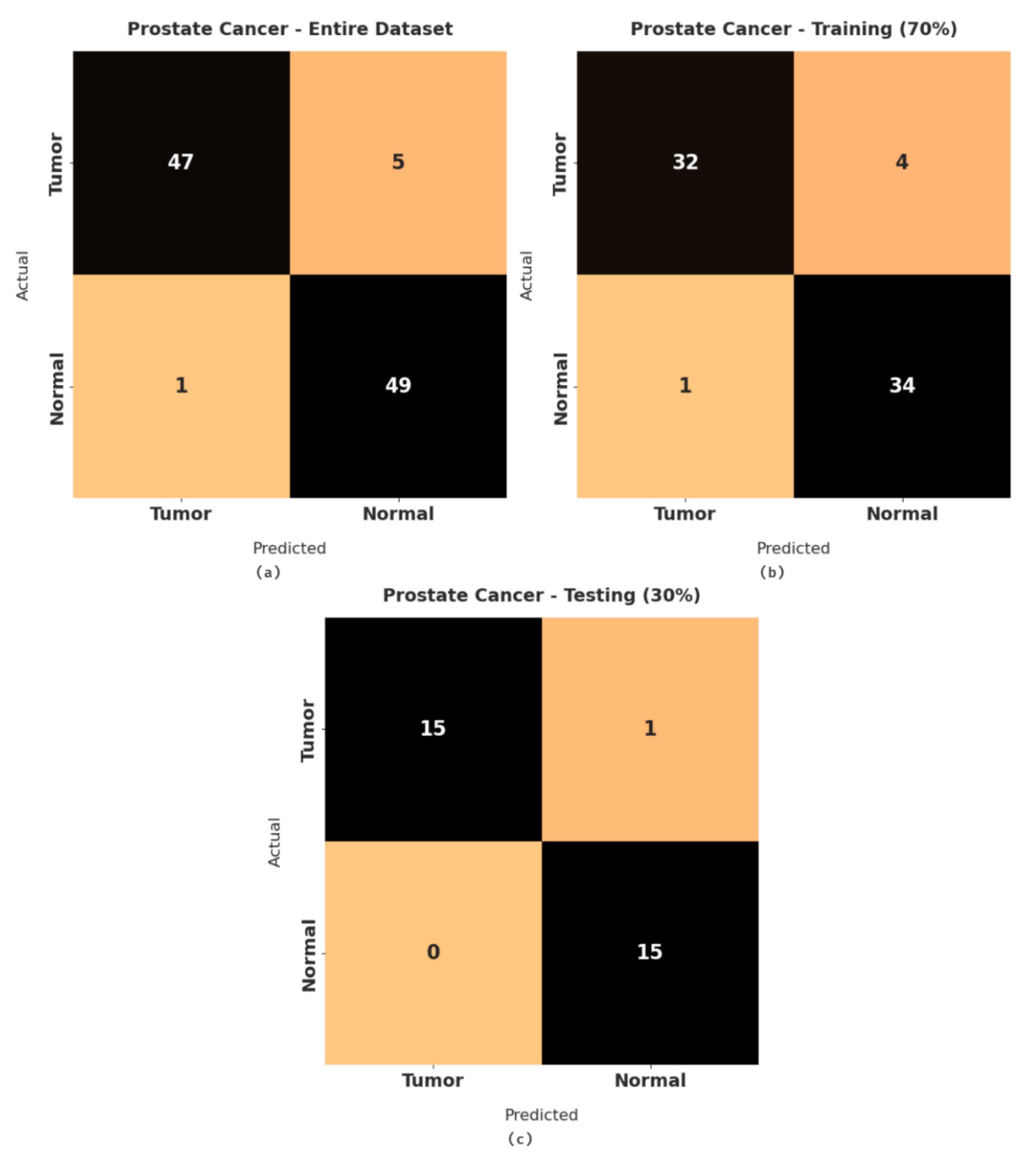
Figure 3 illustrates a set of confusion matrices generated by the RFODL-MGEC model on the test prostate cancer dataset. For the entire dataset, the RFODL-MGEC model categorized 47 images as tumor and 49 images as normal. Similarly, for 70% of the training dataset, the RFODL-MGEC model categorized 32 images as tumor and 34 images as normal. In addition, for 30% of the testing dataset, the RFODL-MGEC model categorized 15 images as tumor and 15 images as normal.

Figure 3. Confusion matrices of RFODL-MGEC technique for prostate cancer dataset. (a) Entire dataset, (b) 70% of training dataset, and (c) 30% of testing dataset.

Table 2 shows a brief classification performance report for the RFODL-MGEC model on the prostate cancer dataset. The experimental results indicated that the RFODL-MGEC model demonstrated effective results on the test dataset. For instance, with the entire dataset, the RFODL-MGEC model obtained an average $acc{u}_y$, $pre{c}_n$, $rec{a}_l$, and $F_{score}$ of 94.12%, 94.33%, 94.19%, and 94.12%, respectively. Moreover, with 70% of the training dataset, the RFODL-MGEC technique obtained an average $acc{u}_y$, $pre{c}_n$, $rec{a}_l$, and $F_{score}$ of 92.96%, 93.22%, 93.02%, and 92.95%, respectively. With 30% of the testing dataset, the RFODL-MGEC system obtained an average $acc{u}_y$, $pre{c}_n$, $rec{a}_l$, and $F_{score}$ of 96.77%, 96.88%, 96.88%, and 96.77%, respectively.

Table 2. Resulting analysis of RFODL-MGEC technique with various measures on prostate cancer dataset.

Prostate Cancer Dataset
Class Labels	Accuracy	Precision	Recall	F-Score
Entire Dataset
Tumor	94.12	97.92	90.38	94.00
Normal	94.12	90.74	98.00	94.23
Average	94.12	94.33	94.19	94.12
Training (70%)
Tumor	92.96	96.97	88.89	92.75
Normal	92.96	89.47	97.14	93.15
Average	92.96	93.22	93.02	92.95
Testing (30%)
Tumor	96.77	100.00	93.75	96.77
Normal	96.77	93.75	100.00	96.77
Average	96.77	96.88	96.88	96.77

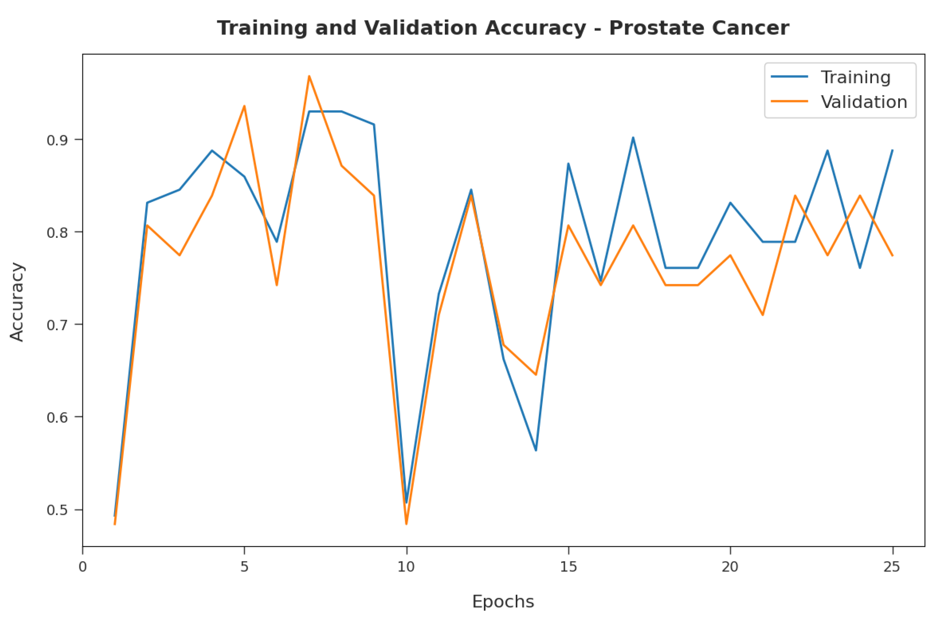
Figure 4 illustrates the training and validation accuracy inspection of the RFODL-MGEC model with the prostate cancer dataset. Figure 4 conveys that the RFODL-MGEC model offered maximum training/validation accuracy for the classification process.

Figure 4. Accuracy analysis of RFODL-MGEC technique on prostate cancer dataset.

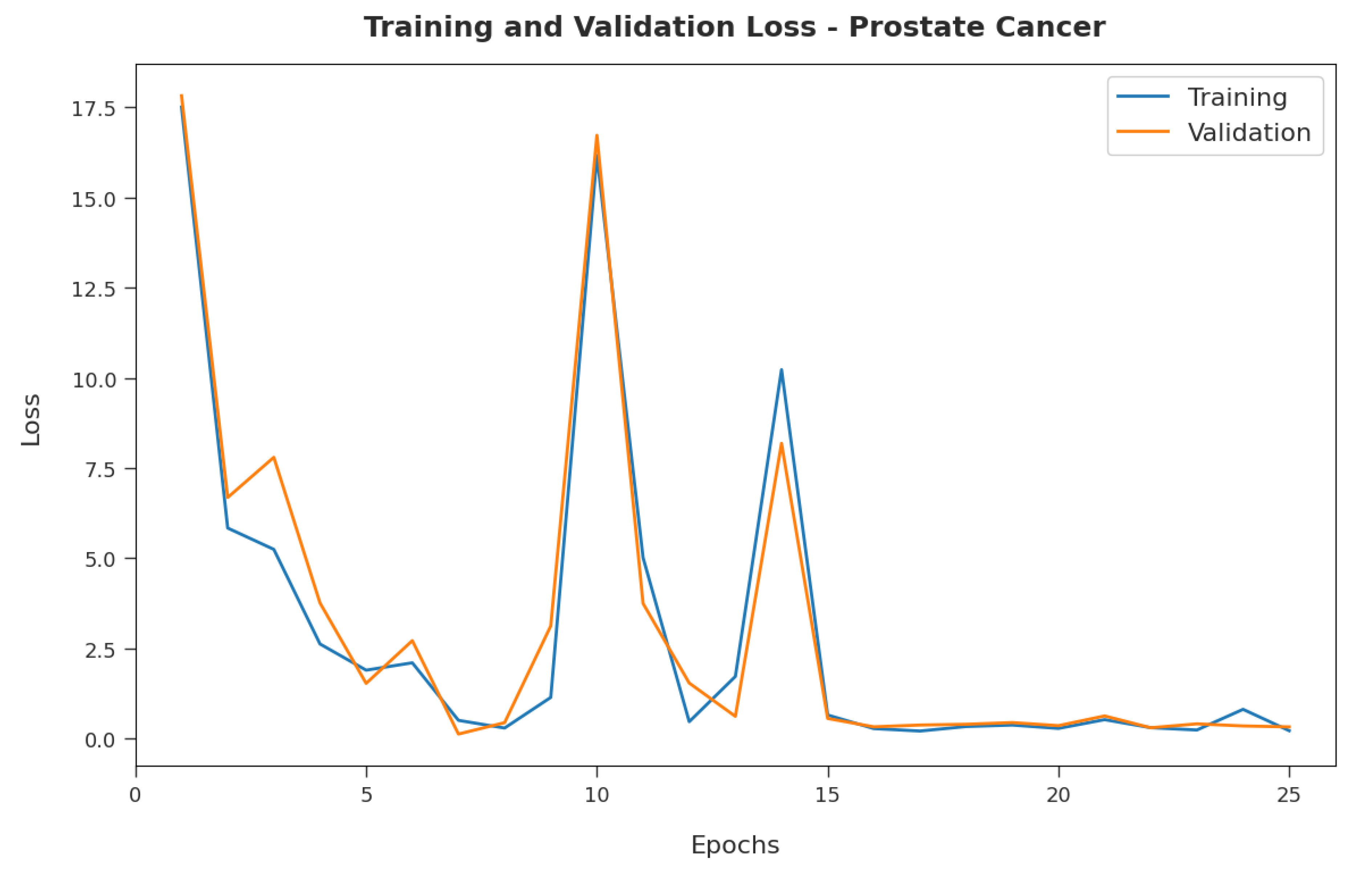
Figure 5 exemplifies the training and validation loss inspection of the RFODL-MGEC model with the prostate cancer dataset. Figure 5 shows that the RFODL-MGEC model offered reduced training/accuracy loss for the classification process of the test data.

Figure 5. Loss analysis of RFODL-MGEC technique on prostate cancer dataset.

4.2. Resulting Analysis of RFODL-MGEC Technique on Colon Tumor Dataset

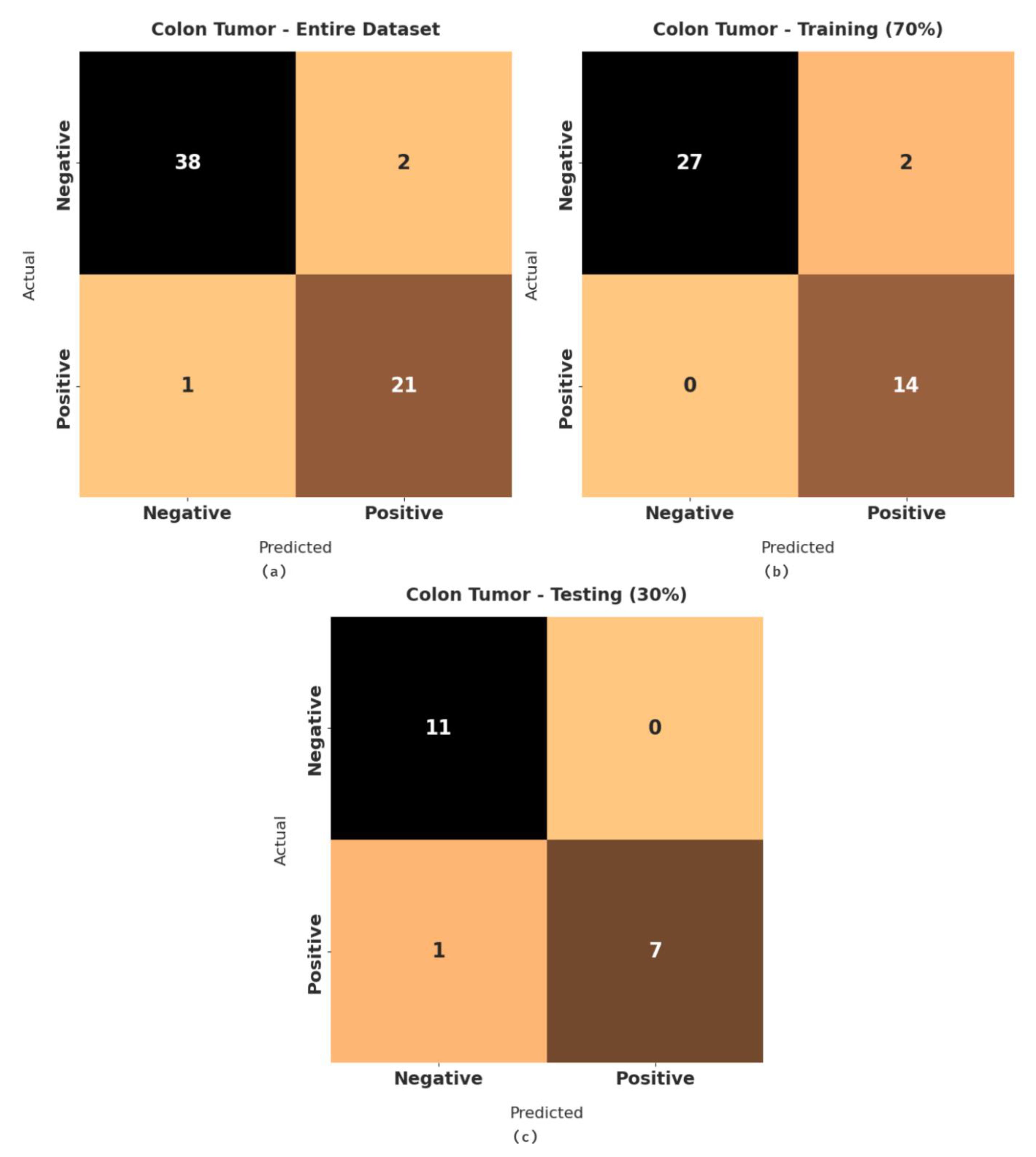
Figure 6 demonstrates a set of confusion matrices generated by the RFODL-MGEC model for the test colon tumor dataset. For the entire dataset, the RFODL-MGEC technique categorized 38 images as negative and 21 images as positive. Likewise, for 70% of the training dataset, the RFODL-MGEC approach categorized 27 images as negative and 14 images as positive. Furthermore, with 30% of the testing dataset, the RFODL-MGEC model categorized 11 images as negative and 7 images as positive.

Figure 6. Confusion matrices of RFODL-MGEC technique on colon tumor dataset. (a) Entire dataset, (b) 70% of training dataset, and (c) 30% of testing datase.

Table 3 demonstrates a brief classification performance report on the RFODL-MGEC model with the colon tumor dataset. The experimental results indicated that the RFODL-MGEC model demonstrated effective results with the test dataset. For instance, with the entire dataset, the RFODL-MGEC model obtained an average $acc{u}_y$, $pre{c}_n$, $rec{a}_l$, and $F_{score}$ of 95.16%, 94.37%, 95.23%, and 94.77%, respectively. With 70% of the training dataset, the RFODL-MGEC method attained an average $acc{u}_y$, $pre{c}_n$, $rec{a}_l$, and $F_{score}$ of 95.35%, 93.75%, 96.55%, and 94.88%, respectively. Additionally, with 30% of the testing dataset, the RFODL-MGEC algorithm obtained an average $acc{u}_y$, $pre{c}_n$, $rec{a}_l$, and $F_{score}$ of 94.74%, 95.83%, 93.75%, and 94.49%, respectively.

Table 3. Resulting analysis of RFODL-MGEC technique with various measures on colon tumor dataset.

Colon Tumor Dataset
Class Labels	Accuracy	Precision	Recall	F-Score
Entire Dataset
Tumor	95.16	97.44	95.00	96.20
Normal	95.16	91.30	95.45	93.33
Average	95.16	94.37	95.23	94.77
Training (70%)
Tumor	95.35	100.00	93.10	96.43
Normal	95.35	87.50	100.00	93.33
Average	95.35	93.75	96.55	94.88
Testing (30%)
Tumor	94.74	91.67	100.00	95.65
Normal	94.74	100.00	87.50	93.33
Average	94.74	95.83	93.75	94.49

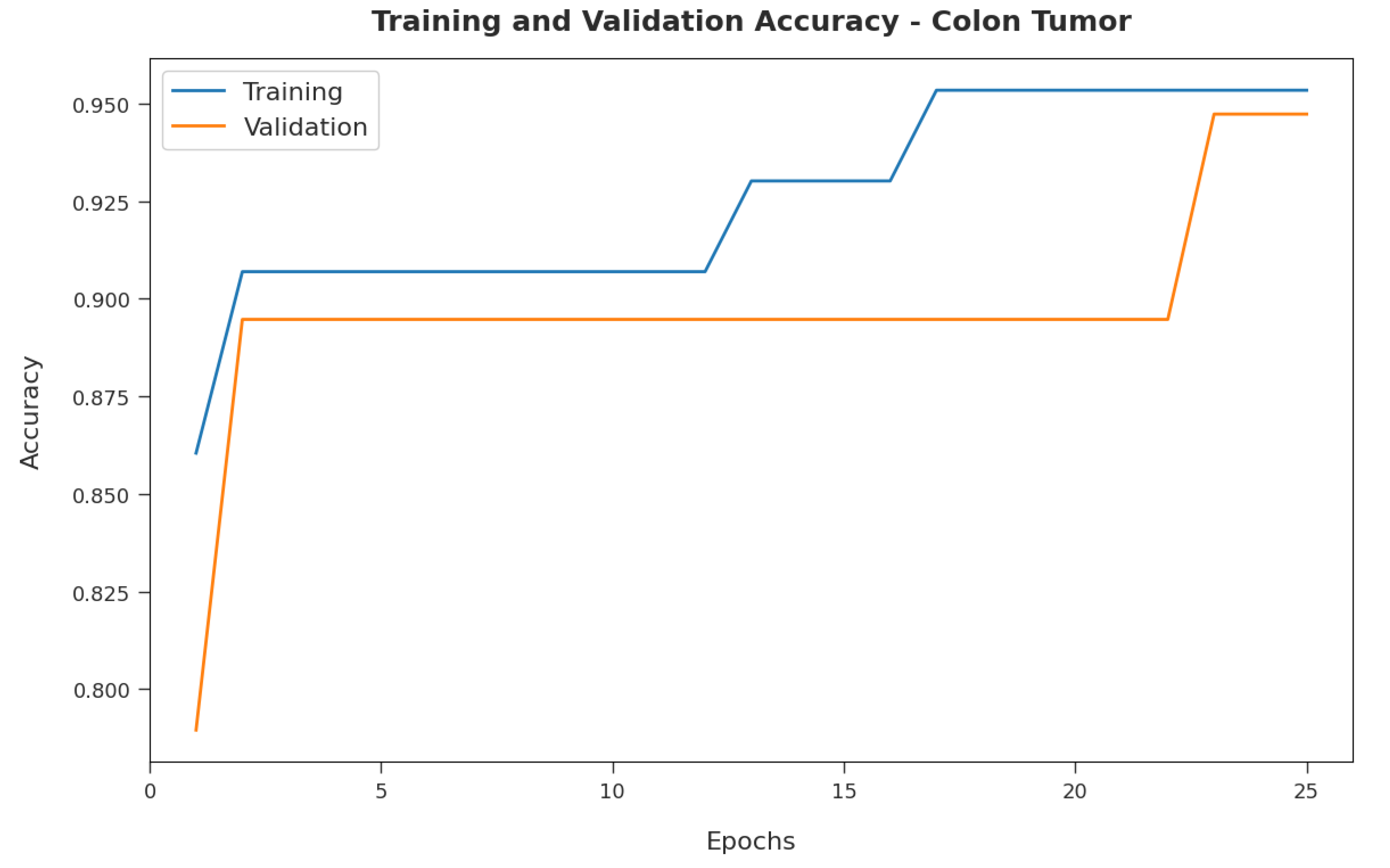
Figure 7 demonstrates the training and validation accuracy inspection of the RFODL-MGEC model on the colon tumor dataset. The figure conveys that the RFODL-MGEC technique offered maximal training/validation accuracy for the classification process.

Figure 7. Accuracy analysis of RFODL-MGEC technique on colon tumor dataset.

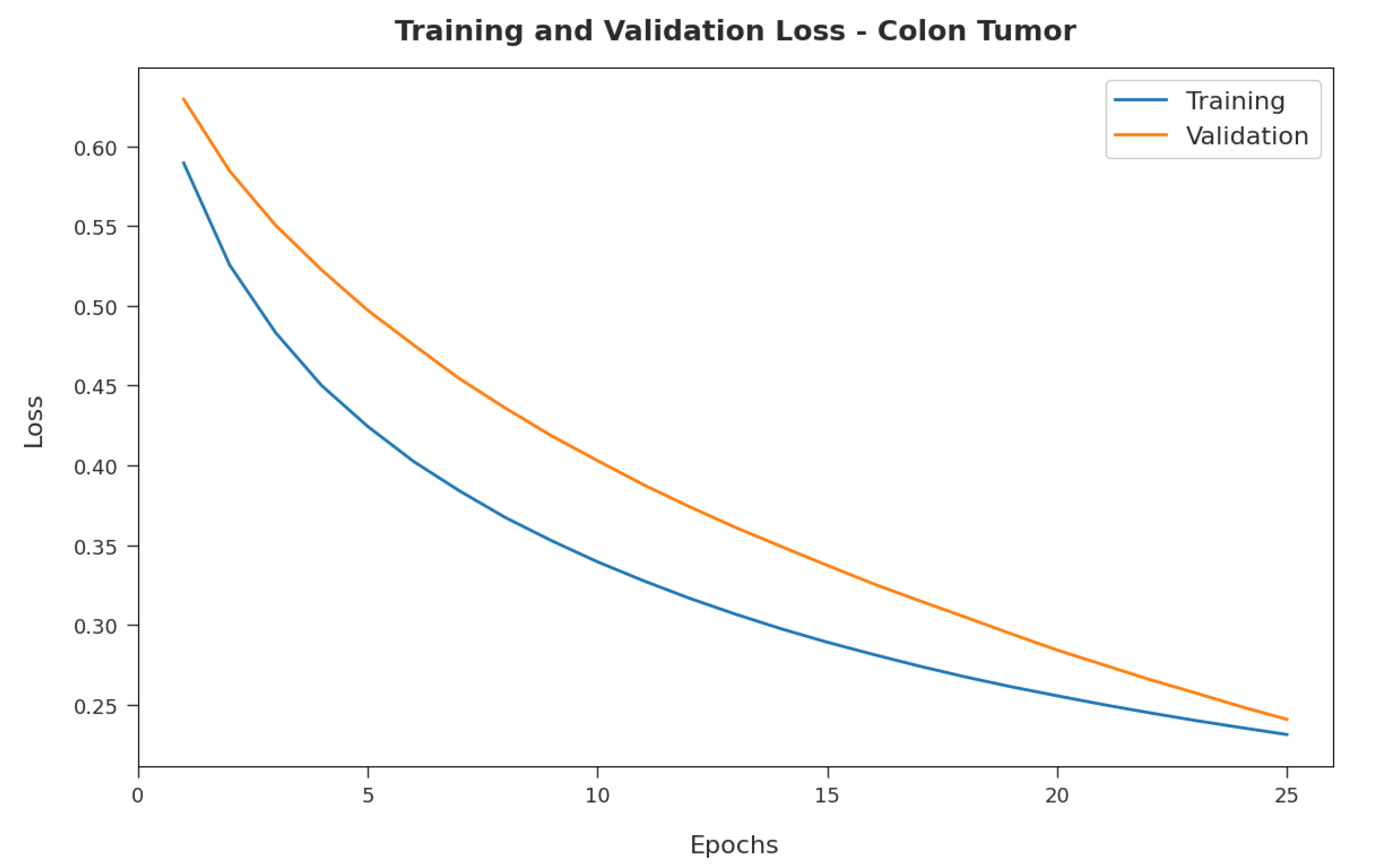
Figure 8 illustrates the training and validation loss inspection of the RFODL-MGEC model on the colon tumor dataset. The figure shows that the RFODL-MGEC approach offered lower training/accuracy loss for the classification process of the test data.

Figure 8. Loss analysis of RFODL-MGEC technique on colon tumor dataset.

4.3. Resulting Analysis of RFODL-MGEC Technique on Ovarian Cancer Dataset

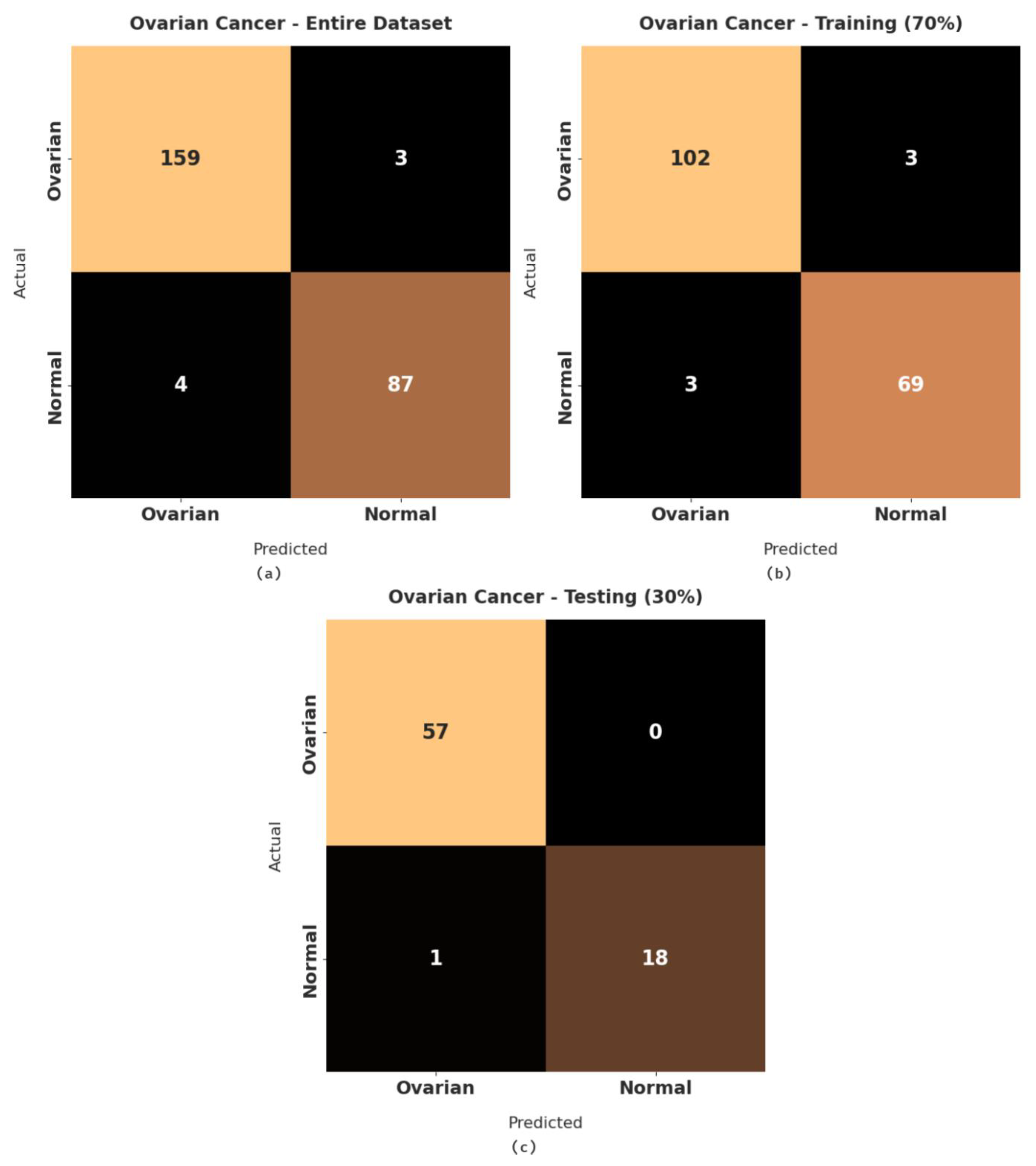
Figure 9 illustrates a set of confusion matrices generated by the RFODL-MGEC algorithm on the test ovarian cancer dataset. For the entire dataset, the RFODL-MGEC technique categorized 159 images as ovarian and 87 images as normal. With 70% of the training dataset, the RFODL-MGEC algorithm categorized 102 images as ovarian and 69 images as normal. For 30% of the testing dataset, the RFODL-MGEC technique categorized 57 images as ovarian and 18 images as normal.

Figure 9. Confusion matrices of RFODL-MGEC technique on ovarian cancer dataset. (a) Entire dataset, (b) 70% of training dataset, and (c) 30% of testing dataset.

Table 4 shows a brief classification performance report on the RFODL-MGEC technique with the ovarian cancer dataset. The experimental results indicated that the RFODL-MGEC technique demonstrated effective results on the test dataset. For instance, with the entire dataset, the RFODL-MGEC system obtained an average $acc{u}_y$, $pre{c}_n$, $rec{a}_l$, and $F_{score}$ of 97.23%, 97.11%, 96.88%, and 96.99%, respectively. With 70% of the training dataset, the RFODL-MGEC algorithm obtained an average $acc{u}_y$, $pre{c}_n$, $rec{a}_l$, and $F_{score}$ of 96.61%, 96.49%, 96.49%, and 96.49%, respectively. Eventually, with 30% of the testing dataset, the RFODL-MGEC algorithm obtained an average $acc{u}_y$, $pre{c}_n$, $rec{a}_l$, and $F_{score}$ of 98.68%, 99.14%, 97.37%, and 98.21%, respectively.

Table 4. Resulting analysis of RFODL-MGEC technique with various measures on ovarian cancer dataset.

Ovarian Cancer Dataset
Class Labels	Accuracy	Precision	Recall	F-Score
Entire Dataset
Tumor	97.23	97.55	98.15	97.85
Normal	97.23	96.67	95.6	96.13
Average	97.23	97.11	96.88	96.99
Training (70%)
Tumor	96.61	97.14	97.14	97.14
Normal	96.61	95.83	95.83	95.83
Average	96.61	96.49	96.49	96.49
Testing (30%)
Tumor	98.68	98.28	100.00	99.13
Normal	98.68	100.00	94.74	97.30
Average	98.68	99.14	97.37	98.21

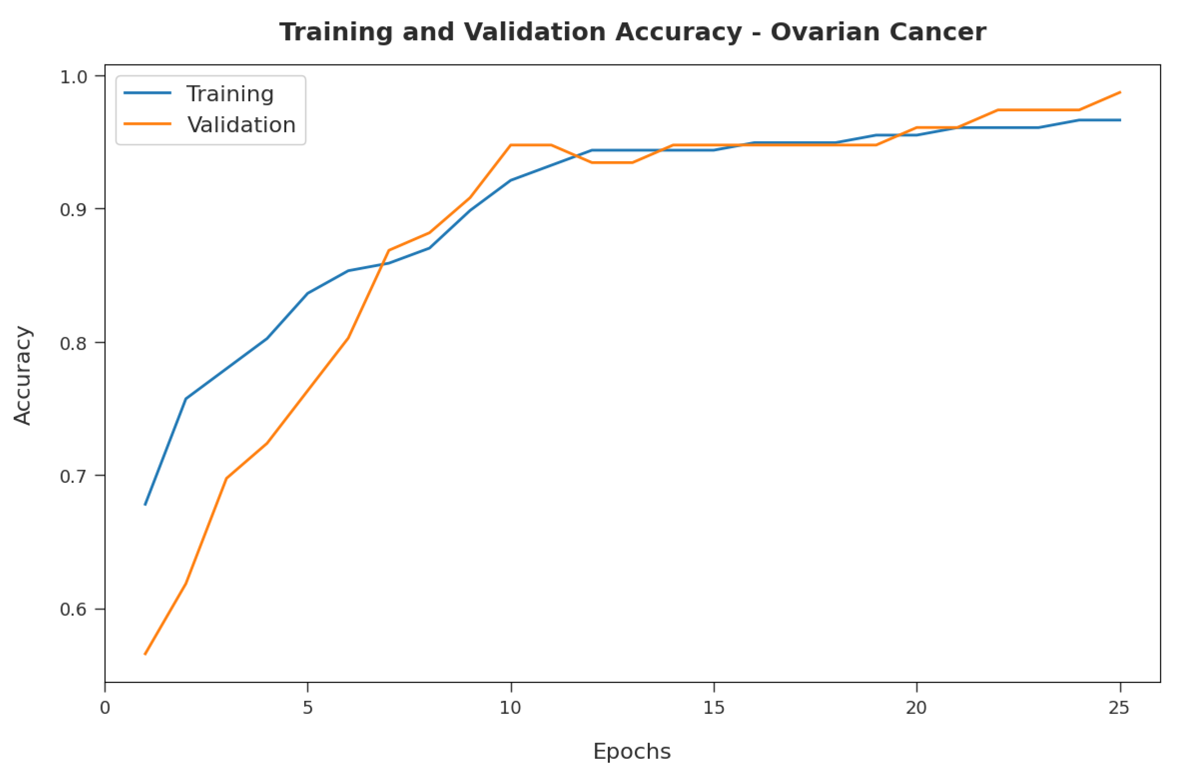
Figure 10 illustrates the training and validation accuracy inspection of the RFODL-MGEC algorithm with the ovarian cancer dataset. The figure conveys that the RFODL-MGEC technique offered maximum training/validation accuracy for the classification process.

Figure 10. Accuracy analysis of RFODL-MGEC technique with ovarian cancer dataset.

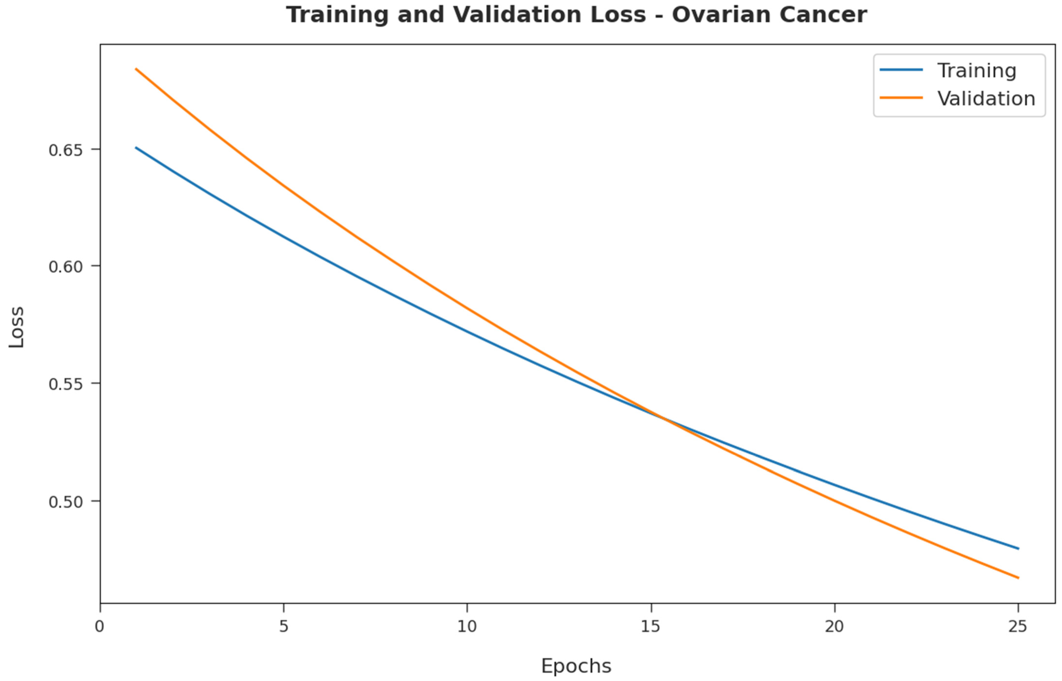
Figure 11 exemplifies the training and validation loss inspection of the RFODL-MGEC technique on the ovarian cancer dataset. The figure shows that the RFODL-MGEC system offered reduced training/accuracy loss for the classification process of the test data.

Figure 11. Loss analysis of RFODL-MGEC technique on ovarian cancer dataset.

4.4. Discussion

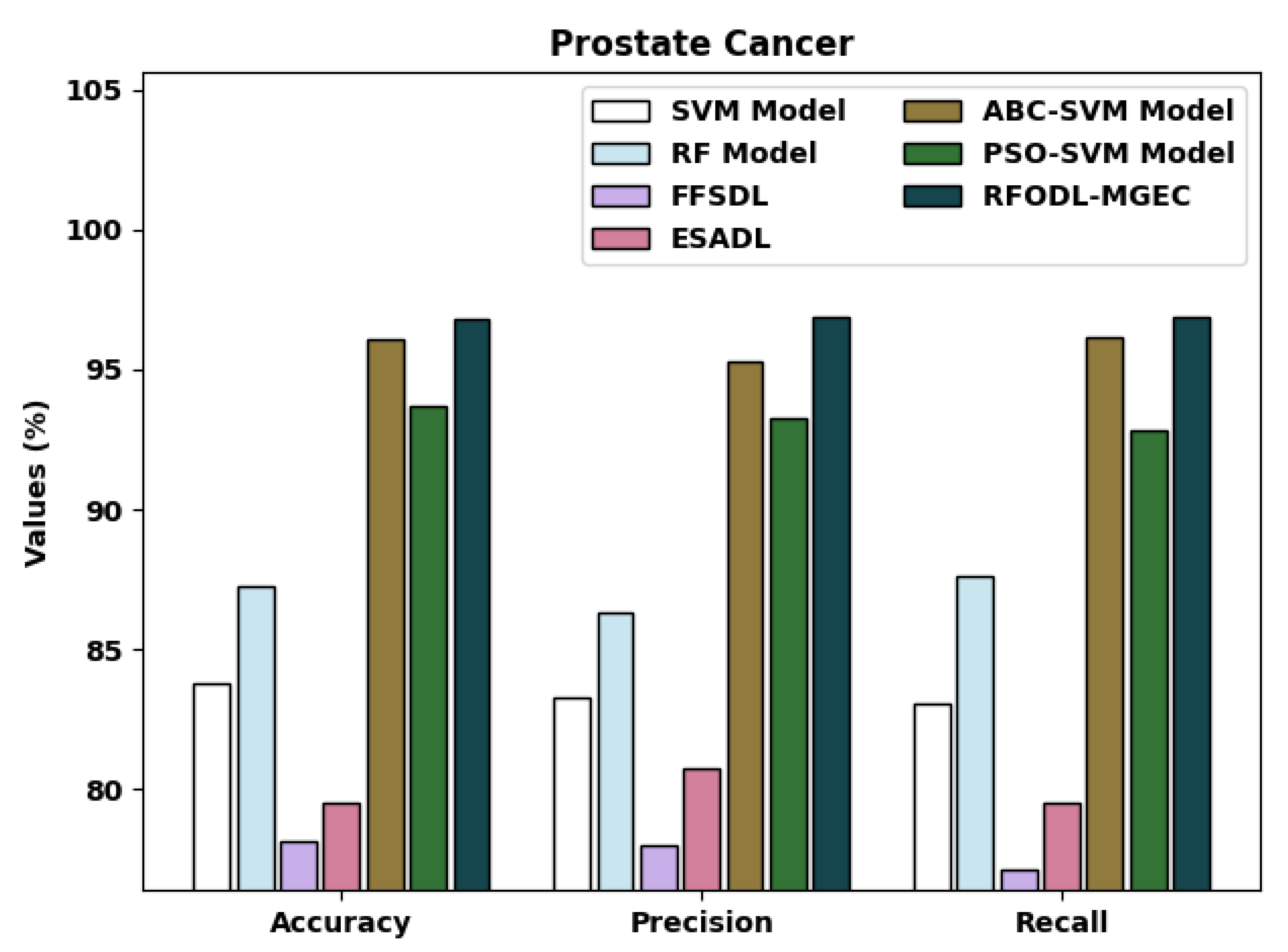
A detailed comparative examination of the RFODL-MGEC model with recent approaches [15] for prostate cancer is provided in Table 5 and Figure 12. The experimental outcomes indicated that the FFSDL and ESADL models reached lower classification outcomes than other approaches. At the same time, the SVM and RF models accomplished slightly enhanced classification outcomes compared with the FFSDL and ESADL models. Along with that, the ABC-SVM and PSO-SVM models accomplished closer classification performances, with an $acc{u}_y$ of 96.06% and 93.71%, respectively.

Table 5. Comparative analysis of RFODL-MGEC technique with recent algorithms for prostate cancer dataset.

Prostate Cancer
Methods	Accuracy	Precision	Recall
SVM Model	83.82	83.26	83.05
RF Model	87.26	86.31	87.61
FFSDL	78.16	78.01	77.16
ESADL	79.51	80.72	79.51
ABC-SVM Model	96.06	95.27	96.15
PSO-SVM Model	93.71	93.23	92.79
RFODL-MGEC	96.77	96.88	96.88

Figure 12. Comparative analysis of RFODL-MGEC technique with prostate cancer dataset.

The proposed RFODL-MGEC model resulted in maximum classification efficiency, with an $acc{u}_y$, $pre{c}_n$, and $rec{a}_l$ of 96.77%, 96.88%, and 96.88% respectively.

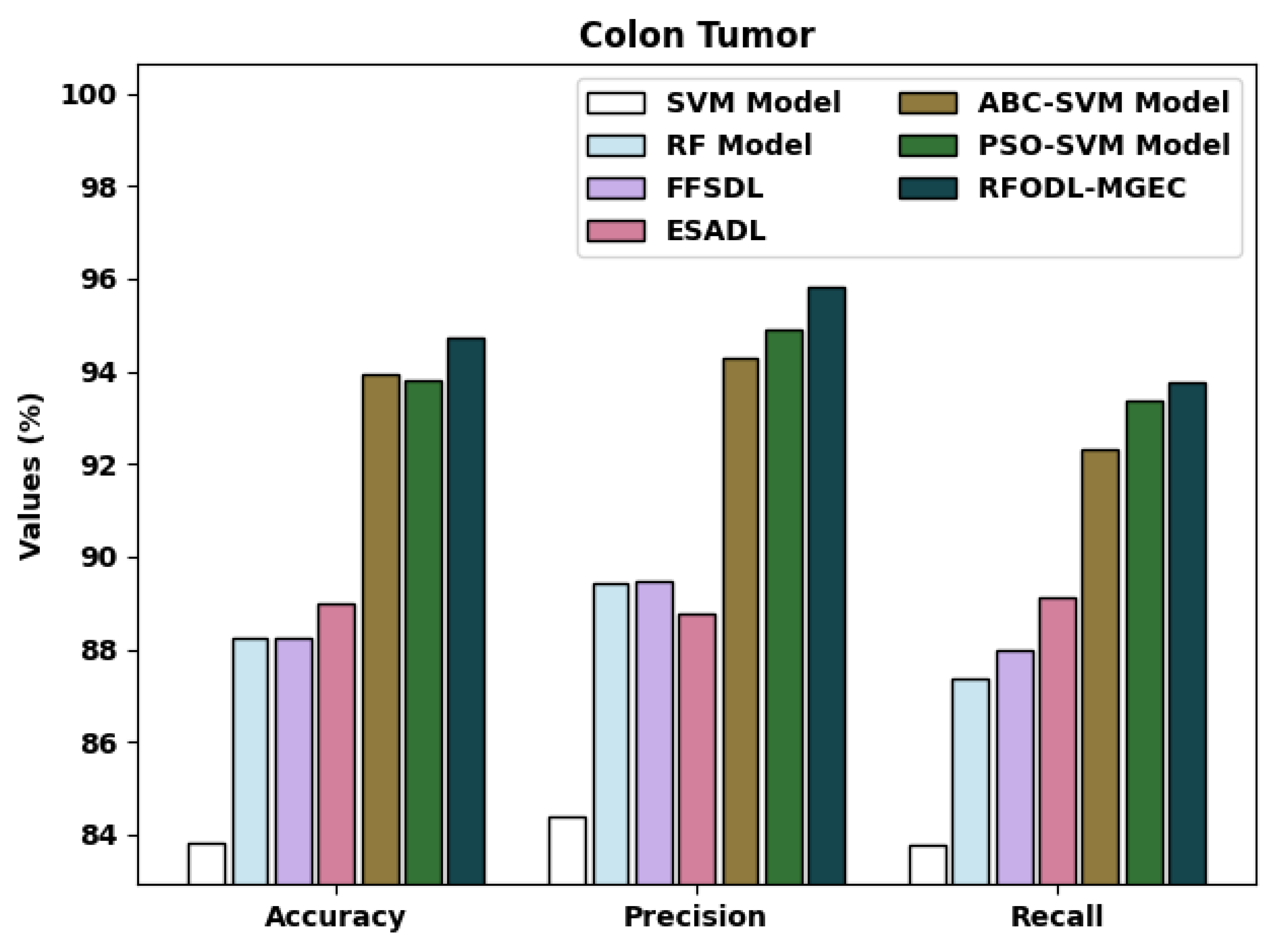
A brief comparative examination of the RFODL-MGEC approach with recent approaches for colon tumors is given in Table 6 and Figure 13. The experimental outcomes indicated that the FFSDL and ESADL approaches reached lower classification outcomes than the other approaches. Likewise, the SVM and RF approaches accomplished somewhat enhanced classification outcomes compared with the FFSDL and ESADL approaches.

Table 6. Comparative analysis of RFODL-MGEC technique with recent algorithms for colon tumor dataset.

Colon Tumor
Methods	Accuracy	Precision	Recall
SVM Model	83.81	84.39	83.77
RF Model	88.26	89.41	87.36
FFSDL	88.26	89.48	87.99
ESADL	88.97	88.77	89.11
ABC-SVM Model	93.94	94.29	92.31
PSO-SVM Model	93.80	94.90	93.37
RFODL-MGEC	94.74	95.83	93.75

Figure 13. Comparative analysis of RFODL-MGEC technique with colon tumor dataset.

Along with that, the ABC-SVM and PSO-SVM models accomplished closer classification performances, with an $acc{u}_y$ of 93.94% and 93.80%, respectively. Finally, the RFODL-MGEC model resulted in higher classification efficiency with an $acc{u}_y$, $pre{c}_n$, and $rec{a}_l$ of 94.74%, 95.83%, and 93.75% respectively.

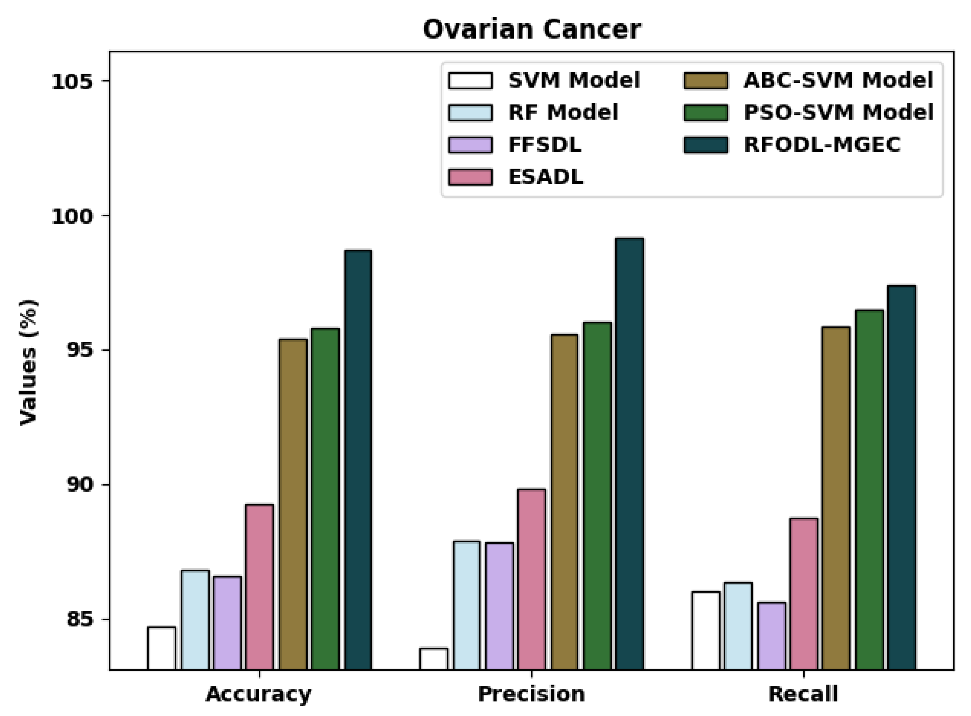
A detailed comparative examination of the RFODL-MGEC algorithm with recent approaches for ovarian cancer is given in Table 7 and Figure 14. The experimental outcomes indicated that the FFSDL and ESADL methods reached lower classification outcomes than the other approaches.

Table 7. Comparative analysis of RFODL-MGEC technique with recent algorithms for ovarian cancer dataset.

Ovarian Cancer
Methods	Accuracy	Precision	Recall
SVM Model	84.71	83.92	85.98
RF Model	86.79	87.86	86.36
FFSDL	86.56	87.82	85.58
ESADL	89.23	89.84	88.74
ABC-SVM Model	95.42	95.56	95.86
PSO-SVM Model	95.81	96.01	96.49
RFODL-MGEC	98.68	99.14	97.37

Figure 14. Comparative analysis of RFODL-MGEC technique with ovarian cancer dataset.

The SVM and RF models accomplished some enhanced classification outcomes compared with the FFSDL and ESADL models. This was followed by the ABC-SVM and PSO-SVM techniques, which accomplished closer classification performances with an $acc{u}_y$ of 95.42% and 95.81%, respectively. Finally, the RFODL-MGEC methodology resulted in maximum classification efficiency, with an $acc{u}_y$, $pre{c}_n$, and $rec{a}_l$ of 98.68%, 99.11%, and 97.37%, respectively.

Finally, a computation time (CT) examination of the RFODL-MGEC technique with recent models for the three distinct datasets is provided in Table 8. The experimental results indicated that the RFODL-MGEC technique showed a lower CT compared with the other methods. The proposed RFODL-MGEC technique required a lower CT of 1.231, 0.432, and 1.542 s with the test prostate cancer, colon tumor, and ovarian cancer datasets, respectively.

Table 8. Comparative CT analysis of RFODL-MGEC technique with recent algorithms.

Computation Time (per s)
Methods	Prostate Cancer	Colon Tumor	Ovarian Cancer
SVM Model	1.903	1.648	1.546
RF Model	1.847	1.640	1.990
FFSDL	1.546	1.462	1.903
ESADL	1.703	0.894	1.094
ABC-SVM Model	1.543	0.452	1.701
PSO-SVM Model	1.656	0.469	1.987
RFODL-MGEC	1.231	0.432	1.542

After examining the aforementioned tables and figures, we noted that the RFODL-MGEC model was able to maximize classification performance compared with the other methods.

5. Conclusions

In this study, a novel RFODL-MGEC model was established for microarray gene expression classification. The presented RFODL-MGEC model primarily employed an RFO-FS technique for deriving an optimal subset of features. Next, the BCDNN model was utilized for data classification, and the parameters involved in the BCDNN technique were optimally tuned by utilizing a CGO algorithm. Comprehensive experiments on benchmark datasets showed that the RFODL-MGEC model accomplished superior results for subtype classifications. Therefore, the RFODL-MGEC model was found to be effective for the identification of different classes for high-dimensional and small-scale microarray data. Future directions involve the use of data clustering and feature reduction approaches to enhance classification performance. The proposed model should be tested on large-scale datasets.

References

1. Ahmed, O.; Brifcani, A. Gene expression classification based on deep learning. In Proceedings of the 2019 4th Scientific International Conference Najaf (SPICN), Al-Najef, Iraq, 29–30 April 2019; pp. 145–149. [Google Scholar]
2. Almugren, N.; Alshamlan, H. A survey on hybrid feature selection methods in microarray gene expression data for cancer classification. IEEE Access 2019, 7, 78533–78548. [Google Scholar] [CrossRef]
3. Maniruzzaman, M.; Rahman, M.J.; Ahammed, B.; Abedin, M.M.; Suri, H.S.; Biswas, M.; El-Baz, A.; Bangeas, P.; Tsoulfas, G.; Suri, J.S. Statistical characterization and classification of colon microarray gene expression data using multiple machine learning paradigms. Comput. Methods Programs Biomed. 2019, 176, 173–193. [Google Scholar] [CrossRef] [PubMed]
4. Tabares-Soto, R.; Orozco-Arias, S.; Romero-Cano, V.; Bucheli, V.S.; Rodríguez-Sotelo, J.L.; Jiménez-Varón, C.F. A comparative study of machine learning and deep learning algorithms to classify cancer types based on microarray gene expression data. PeerJ Comput. Sci. 2020, 6, e270. [Google Scholar] [CrossRef] [PubMed] [Green Version]
5. Adiwijaya, W.U.; Lisnawati, E.; Aditsania, A.; Kusumo, D.S. Dimensionality reduction using principal component analysis for cancer detection based on microarray data classification. J. Comput. Sci. 2018, 14, 1521–1530. [Google Scholar] [CrossRef] [Green Version]
6. Alanni, R.; Hou, J.; Azzawi, H.; Xiang, Y. A novel gene selection algorithm for cancer classification using microarray datasets. BMC Med. Genom. 2019, 12, 10. [Google Scholar] [CrossRef] [PubMed]
7. Daoud, M.; Mayo, M. A survey of neural network-based cancer prediction models from microarray data. Artif. Intell. Med. 2019, 97, 204–214. [Google Scholar] [CrossRef] [PubMed]
8. Aydadenta, H.; Adiwijaya, A. A clustering approach for feature selection in microarray data classification using random forest. J. Inf. Process. Syst. 2018, 14, 1167–1175. [Google Scholar]
9. Cilia, N.D.; De Stefano, C.; Fontanella, F.; Raimondo, S.; Scotto di Freca, A. An experimental comparison of feature-selection and classification methods for microarray datasets. Information 2019, 10, 109. [Google Scholar] [CrossRef] [Green Version]
10. Alhenawi, E.A.; Al-Sayyed, R.; Hudaib, A.; Mirjalili, S. Feature selection methods on gene expression microarray data for cancer classification: A systematic review. Comput. Biol. Med. 2022, 140, 105051. [Google Scholar] [CrossRef] [PubMed]
11. Wang, H.; Tan, L.; Niu, B. Feature selection for classification of microarray gene expression cancers using Bacterial Colony Optimization with multi-dimensional population. Swarm Evol. Comput. 2019, 48, 172–181. [Google Scholar] [CrossRef]
12. Zeebaree, D.Q.; Haron, H.; Abdulazeez, A.M. Gene selection and classification of microarray data using convolutional neural network. In Proceedings of the 2018 International Conference on Advanced Science and Engineering (ICOASE), Duhok, Iraq, 9–11 October; pp. 145–150.
13. Algamal, Z.Y.; Lee, M.H. A two-stage sparse logistic regression for optimal gene selection in high-dimensional microarray data classification. Adv. Data Anal. Classif. 2019, 13, 753–771. [Google Scholar] [CrossRef]
14. Shukla, A.K.; Singh, P.; Vardhan, M. A two-stage gene selection method for biomarker discovery from microarray data for cancer classification. Chemom. Intell. Lab. Syst. 2018, 183, 47–58. [Google Scholar] [CrossRef]
15. Panda, M. Elephant search optimization combined with deep neural network for microarray data analysis. J. King Saud Univ. Comput. Inf. Sci. 2020, 32, 940–948. [Google Scholar] [CrossRef]
16. Sayed, S.; Nassef, M.; Badr, A.; Farag, I. A nested genetic algorithm for feature selection in high-dimensional cancer microarray datasets. Expert Syst. Appl. 2019, 121, 233–243. [Google Scholar] [CrossRef]
17. Li, Z.; Xie, W.; Liu, T. Efficient feature selection and classification for microarray data. PLoS ONE 2018, 13, e0202167. [Google Scholar] [CrossRef] [PubMed]
18. Khorami, E.; Mahdi Babaei, F.; Azadeh, A. Optimal diagnosis of COVID-19 based on convolutional neural network and red Fox optimization algorithm. Comput. Intell. Neurosci. 2021, 2021, 4454507. [Google Scholar] [CrossRef] [PubMed]
19. Kong, W.; Chen, J.; Huang, Z.; Kuang, D. Bidirectional cascaded deep neural networks with a pretrained autoencoder for dielectric metasurfaces. Photonics Res. 2021, 9, 1607–1615. [Google Scholar] [CrossRef]
20. Talatahari, S.; Azizi, M. Chaos Game Optimization: A novel metaheuristic algorithm. Artif. Intell. Rev. 2021, 54, 917–1004. [Google Scholar] [CrossRef]
21. Zhu, Z.; Ong, Y.S.; Dash, M. Markov Blanket-Embedded Genetic Algorithm for Gene Selection. Pattern Recognit. 2007, 49, 3236–3248. Available online: http://csse.szu.edu.cn/staff/zhuzx/Datasets.html (accessed on 21 January 2022). [CrossRef]
Publisher’s Note: MDPI stays neutral with regard to jurisdictional claims in published maps and institutional affiliations.
Article Metrics
Citations
Article Access Statistics
Multiple requests from the same IP address are counted as one view.