Numerical Voids Detection in Bonded Metal/Composite Assemblies Using Acousto-Ultrasonic Method

Abstract

This research focuses on the application of an acousto-ultrasonics (AU) technique, a combination of ultrasonic characterization and acoustic emission, to nondestructively detect defects such as voids in bonded metal/composite assemblies. Computational methods are established to examine the effects of voids on the collected signal. The position of the receiver sensor with respect to the defect is also investigated. Given a specific structure and type of actuation signal, the sensor location and probability of detection can be enhanced by the model developed in this work. The defect detection is optimal provided the receiver sensor is located around the epicenter of the defect. Moreover, this work highlights the importance of the choice of reception sensor.

1. Introduction

Composite materials are increasingly used as bonded reinforcements on civil engineering structures, owing to their lightness and durability [1,2,3]. Adhesive bonding enables physically dissimilar materials such as composites and metals to be joined. Used in the repair, reinforcement and rehabilitation of structures with composites, this extends the service life of structures. Despite their advantages, the effectiveness of bonded joints can be compromised due to the presence of adhesion defects or damage such as voids, porosity, poor adhesion or low cohesion strength. Accordingly, non-destructive testing (NDT) techniques [4,5,6,7] become essential for damage or defect diagnosis using actuators/sensors installed on the same side of the structure. Defects need to be identified either during initial control or by inspection during service life. The mechanical joint behavior may be significantly impacted by the defects [8,9]. Substantial efforts have been made to develop nondestructive testing methods to evaluate the adhesive bond integrity. Several investigations focused on adhesive joint quality inspections using ultrasonic testing methods including acoustic emission, bulk and guided (longitudinal, shear and Lamb) waves, shearography, pulsed thermography, X-rays or passive thermography [10,11,12,13,14,15,16,17]. For example, Yilmaz et al. [11] compared the performance of different ultrasonic non-destructive testing (contact testing, immersion testing and air-coupled) techniques for bonding quality evaluation on aluminum–epoxy–single lap joints containing debonding in the form of release film inclusions. Yang et al. [12] used damping and frequency measurements to monitor a kissing-bond defect in an adhesively bonded joint between two composite strips. The results showed a nonlinear relation between the defect area and modal damping as well as frequency variations. Wang et al. [15] evaluated the damage in an aluminum plate with a carbon fiber reinforced polymer (CFRP) using the amplitude change of the second-order harmonic waves with nonlinear acousto-ultrasonic detection. Le Crom et al. [16] demonstrated the strong potential of the low-order SH₀- and SH₁-like guided modes to quantify the shear properties of adhesive bond layers between an aluminum plate and a carbon epoxy composite patch. The precise monitoring of structures with composite repairs is also challenging. It is important to detect and locate a defect, to determine its size, to classify its type and to evaluate its severity.

In this context, several authors proposed the use of an acousto-ultrasonic (AU) method [18,19,20,21,22,23,24,25,26,27] to detect and assess defects. This technique was initially introduced and developed by Vary [18] and was rapidly used to characterize bonding [19,20,21,22]. Indeed, Tanary [21,22] used the acousto-ultrasonic technique to nondestructively evaluate the mechanical performance of composite bonded joints. A good correlation between the acousto-ultrasonic wave propagation characteristics and the bonded joint shear strength was established. The monitoring principle, based on an actuator-sensor configuration, is quite similar that used in standard guided ultrasonic inspection. In the AU approach, it is not necessary to have well-defined wave propagation paths. On the contrary, the approach requires that the transmitter signal presents multiple interactions with the microstructure of the material. Moreover, this technique allows an active (emission of AU) and a passive phase to be combined with acoustic emission (AE) monitoring. This technique can combine advantageous aspects of both acoustic emission and ultrasonic techniques. Additionally, it requires the sensors to be located on only one side of the specimen. The acousto-ultrasonic technique (AU) consists of emitting an ultrasonic wave with a piezo ceramic transducer and receiving the wave after its propagation in the material using a similar transducer with an AE acquisition system. The recorded wave is then analyzed using acoustic emission descriptors. This technique works in a frequency domain similar to that used in acoustic emission. Furthermore, damage detection requires knowledge of the structure in its undamaged state. The baseline data or reference signals are obtained from the undamaged state. The damage detection is then performed by comparing the received signal descriptors from the tested specimen with those of the baseline signals. Kwon and Lee [23] investigated the correlation between the number of delamination-type defects and the acousto-ultrasonic parameters in an aluminum–composite bonded assembly, mainly using frequency parameters based on a spectral study of the detected signals. Barile et al. [25,26] used AU measurements to characterize the interlaminar strength of CFRP laminates in both longitudinal and transverse directions and to study the integrity of CFRP specimens before and after artificially induced, barely visible impact damage.

This method, as the standard guided ultrasonic inspection method, is based on the interaction of the waves with the defects present in the adhesive joint. The main difference is that the wave modes and propagation paths are not well established. The signal is therefore difficult to analyze; nevertheless, it is a rich source of information that reflects the material properties, microstructure and possible presence of defects. A single experimental approach is thus not sufficient to fully understand this interaction. Compared with experimental techniques, numerical analyses can offer a more comprehensive study of wave propagation and interactions with defects in the joint. Analytical solutions for wave propagation are generally limited to infinite media or simple geometries and are therefore not accessible for most practical structures. The wave propagation solution can be approximated using numerical approaches such as finite element (FE) analysis. Three-dimensional FE approaches are beneficial, since they enable a realistic structure geometry to be considered, as well as material anisotropy or wave reflections at boundaries.

Several authors [16,27,28,29,30,31,32,33] focused on the modeling of wave propagation in bonded assemblies to predict the ultrasonic response. All these studies showed the defect sensitivity of various guided wave modes propagating in adhesively bonded joints and demonstrated the potential of modeling studies. Crom and Castaings [16] developed a one-dimensional semi-analytical FE model for predicting dispersion curves and mode shapes of SH-guided waves in multilayered plates made of composite and adhesive layers. Numerical simulations were used for selecting the most appropriate SH wave modes with higher sensitivity to the bond than to the other components (the metallic plate or composite patch). Some authors [31] used the global matrix method to model wave propagation in the multilayer overlap and showed that phase and group velocity dispersion curves are highly sensitive to the bond state and bonded lap–shear joints. The study in [28] investigated two different lay-ups for the wing skin and two different types of bond defects (poorly cured adhesive and debonded interfaces). The models and the experiments confirmed that the ultrasonic energy transmission through the joint is highly dependent on the bond conditions. Using FE simulations for each of the modes A₀, S₀ and A₁, Lowe et al. [29] predicted the transmission coefficient of each mode across a lap joint consisting of parallel aluminum sheets bonded with an epoxy adhesive. Koreck et al. [32] used computational methods to examine the properties of double-layered, adhesive-bonded plates. They quantified the influence of adhesive bond parameters (Young’s modulus, Poisson’s ratio and bond thickness) on the dispersion curves. Vaziri et al. [33] proposed a model to investigate the influence of a void in the overlap area and showed that modal damping decreased with increasing void size. Janapati et al. [27] identified critical parameters for the damage detection sensitivity via numerical simulations using a spectral-element-model-based analysis and experimental results obtained from aluminum coupons. Their results indicated that the uncertainty in the sensor–transmitter installation and the damage propagation path have a significant effect on the recorded signals and the damage index evaluation. Wave propagation was also simulated in the context of acoustic emission [34,35,36,37,38,39,40,41,42,43], where the source was not a controlled emission signal but originated from a damage mechanism occurring in the material. Since both AU and AE techniques use the same acquisition system and the same sensors, wave propagation modeling [34,35,36,40,41,42,43] and receiver sensor modeling [37,38,39,44] are equivalent. The AE source modeling is, however, quite different from models developed in acoustics, since the sources (for instance, crack propagation) are not controlled in the AE analysis. Although the literature in the field of acoustic emission modeling is relatively significant, few authors simulated wave propagation in the context of AU.

In a previous paper [24] concerning the experimental characterization of metal/composite or concrete/composite assemblies using AU, we showed that the identification of this kind of defect is quite difficult. Nevertheless, the proposed methodology proved to be sensitive to all the studied defects in two different bonded assemblies. Therefore, more investigations are necessary to define the limits of the method. In order to increase the robustness of the technique, a more quantitative approach based on modeling work is required in order to quantify the defect influence on wave propagation through the assembly and the corresponding acquired signals.

This paper deals with numerical AU simulations in assemblies made of a steel substrate and a unidirectional composite laminate bonded with an epoxy adhesive. The objective of this work is to investigate numerically the sensitivity of the AU technique to voids within the joint. Three-dimensional FE models are developed to simulate the influence of voids and sensor location on the recorded signal. The paper is structured as follows. The experimental and numerical approaches are presented in Section 2 and Section 3. In Section 4, we study the received signals obtained with two kinds of sensors, a perfect sensor and an R15 sensor, and highlight the influence of the receiver sensor location on the composite plate.

2. Materials and Experimental Setup

This section describes the experimental setup [24].

2.1. Samples

The investigated geometry, which consisted of a steel substrate and a composite plate bonded together by an epoxy adhesive layer, is shown in Figure 1. The composite (T800 S carbon fibers and epoxy matrix) and adhesive layer dimensions were 300 mm × 50 mm with thicknesses of 1.4 mm and 1 mm, respectively. The steel substrate (dimensions 320 mm × 100 mm) was 5 mm thick. A two-component cold-curing epoxy resin (Sikadur 30) was employed as the adhesive. The properties of the materials are summarized in

Table 1. Composite, steel and epoxy properties.

	Longitudinal Young’s Modulus (GPa)	Transversal Young’s Modulus (GPa)	Longitudinal Poisson’s Ratio	Longitudinal Shear Modulus (GPa)	Transverse Poisson’s Ratio	$\mathbf{Density}(\mathbf{g}/\mathbf{c}{\mathbf{m}}^3)$
Steel S355	210.00	210.00	0.24–0.30	-	-	7.85
Composite (FLT M514)	210.00	15.33	0.25	5.50	0.25	1.67
Adhesive joint epoxy (Sikadur 30)	12.80	12.80	0.29–0.34	-	-	1.95 at 20 °C

. Figure 1 also indicates the location of the voids. The reference sample, with no voids in the adhesive layer, was denoted the α-type sample. For the β samples, a void was present in the middle of the adhesive bond line. The void defects had two different sizes. A β1-type defect was simulated with a lack of adhesive on a central area of dimensions 50 × 25 mm², and a β2-type defect corresponded to a lack of adhesive on 1/3 of the bonded surface at the center of the joint (100 × 50 mm²). The assemblies were instrumented with 3 sensors located on the composite plate.

2.2. Acousto-Ultrasonic Technique

An ARB-1410 arbitrary waveform generator card and an AE PCI-2 receiving card, commercialized by the MISTRAS group, were used (Mistras Group, Princeton, NJ, USA). The signal applied to the piezoelectric sensor acting as the actuator corresponded to a continuous square signal with a frequency of 150 kHz. An S9204 sensor in emission mode with a bandwidth centered at 150 kHz and two R15 sensors as receivers with a 150 kHz resonance frequency (Mistras Group, Princeton, NJ, USA) were used. The sensors (transmitter and receivers) were placed on the composite plate so that they were aligned along the composite fiber direction. Sensor 2 (receiver) was located in the center of the composite plate. On the β specimens, this location corresponded to the location of the defect center. Sensor 1 (receiver) was located opposite to sensor T (the transmitter) with respect to the middle plane of the specimen. This arrangement is illustrated in Figure 2a. A low-melting-point crystal, phenyl salicylate, was used as the coupling between the sensors and the specimens. To acquire signals with a gain of 40 dB, we used an IL40S-HT preamplifier with a 32–1100 kHz band-pass filter. The recording threshold was set to 45 dB. For repeatable AU measurements, test conditions such as temperature, sensor location, spacing and type of coupling were kept constant. To simulate the effects of the mounting procedure and to consider the induced uncertainty, seven independent measurements were completed. Each series of measurements was composed of 10 shots. For the propagated signals recorded with the AE acquisition system, several features could be extracted from the signal, for instance, the amplitude or frequency centroids.

3. Model Description

A 3D FE model was set up using Abaqus commercial software (Dassault Systèmes Simulia Corp., Providence, RI, USA).

3.1. Simulation of the Source and the Propagation Medium

The assembly was modeled by three layers corresponding to the steel substrate, the composite plate and the epoxy joint. The behavior of each layer was assumed to be linearly elastic. The excitation was simulated by an imposed displacement equal to 0.01 mm at one of the mesh nodes corresponding to the emitting sensor (T) center location (Figure 2b). The calculation was performed in two steps. During the first step, an input signal was generated at the emitting sensor location, then in the second step the resulting acoustic wave propagated in the assembly. The input signal was defined as a 150 KHz sinusoidal signal consisting of 3 periods, with a total duration of 2.00 × 10⁻⁵ s. This signal is idealized because it is not experimentally straightforward to control the signal emitted by a sensor (S9204), where sensitivity in emission is expected to influence the output signal. Therefore, it is difficult to achieve a quantitative comparison of numerical simulations with experimental results. Nevertheless, working with an idealized sinusoidal source at emission enables the influence of the receiver sensor type and location to be studied, as well as the presence of a defect, for a given signal. For the wave propagation simulation, a total time period of 2.80 × 10⁻⁴ s and a time step of 3.30 × 10⁻⁷ s were used. The material damping was described by the Rayleigh coefficients α and β [39,40,41,42,43]. Their values for epoxy and carbon fiber composite were taken from the literature [42,43]. For steel, we calculated the damping coefficients α and β using Equation (1) in order to obtain the known damping coefficient (ξ) at a given frequency.

$$\xi =\frac{\alpha }{2\omega }+\frac{\beta \omega }{2}$$

(1)

where $\omega$ is the pulsation.

Table 2. Rayleigh parameters.

	$\mathit{\alpha } \left({\mathbf{s}}^{-1}\right)$	$\mathit{\beta } \left(\mathbf{s}\right)$
Steel	500	$4·{10}^{-10}$
Composite [43]	10,000	$6·{10}^{-10}$
Epoxy [43]	50,000	${10}^{-8}$

summarizes the values of α and β for the studied materials. Linear 3D elements with 8 nodes were selected. In order to determine the mesh size, a convergence study was performed. Based on this study, a 2 mm mesh size was selected. It was ensured that 20 elements existed per wavelength. Acoustic excitation at 150 kHz was sent by the emitting sensor through the assembly, and the propagated signals were determined by calculating the out-of-plane displacements at specific locations on the assembly surface.

3.2. Simulation of the Receiver Sensor

Several receiver sensor distances from the emitting sensor were investigated, from 28 mm to 230 mm (Figure 2b). The sensors were assumed to be sensitive only to the out-of-wave plane velocity or displacement. Two kinds of sensors were simulated: a perfect point sensor denoted PS and an R15 sensor. The perfect sensor is a virtual sensor that acquires signals at a single measurement point (a node) without averaging effects and is sensitive to all frequencies. A real sensor has a contact surface with the sample that must be considered. The R15 sensor consists of a piezoelectric ceramic with a 7.25 mm radius. Moreover, the sensor has an aperture effect, which results in a non-uniform response over its entire active surface (Figure 3a). It has its maximum sensitivity at its center. Sensitivity is described by the parameter k, which represents the sensitivity of a point at a distance r from the center of the sensor surface. It is given by Equation (2) [42]:

$$k\left(r\right)=1-\frac{1}{1+ex{p}^{\left(-2r+12\right)}}$$

(2)

The influence of the physical sensor is considered by calculating an average out-of-plane wave velocity over the sensor surface (S), accounting for its sensitivity:

$$V_s=\frac{1}{{{\displaystyle \int }}_{S}kdS}{{\displaystyle \int }}_{S}vkdS$$

(3)

In practice the average wave velocity is approximated by a discrete sum over the velocities $v$ calculated at the mesh nodes. The frequency sensitivity of the sensor must also be considered. The frequency sensitivity function of the R15 sensor as a receiver is given in Figure 3b. The calibration curve is obtained by the reciprocity method [44]. Its bandwidth is centered on 50–400 kHz. This transfer function is added in the post-processing phase in the Fourier domain, following Equation (4):

$$V_s\left(\omega \right)\times H_{R15}\left(\omega \right)=V_{R15}\left(\omega \right)$$

(4)

where V_R15 is the velocity calculated considering the sensor, V_s (ω) represents the weighted mean out-of-plane velocity on the surface, H_R15 (ω) is the sensitivity function and $\omega$ is the pulsation. In this study, the coupling medium was not considered. All numerical velocity signals were filtered with a 20 kHz to 1200 kHz Butterworth band-pass filter. Several sensor locations between 28 mm and 230 mm from the transmitter were analyzed (Figure 2b).

3.3. Analysis of the Experimental and Simulated Signals

The end of the experimentally acquired signals was determined using an energy criterion. At each point of the experimental signal, the cumulative energy from the fixed threshold was compared to the energy contained in the 10 µs interval following the considered point. If the energy contained in the time interval was smaller than 0.1% of the cumulative energy, the point indicated the end of the signal [45].

For numerical signals, an energy criterion was also used to define the signal beginning and end using a criterion of 0.1% of the energy for the beginning and 99.9% of the energy for the end. The main extracted descriptors analyzed were the following: signal amplitude, duration, centroid frequency and peak frequency.

4. Results and Discussion

4.1. Summary of the Experimental Results

Figure 4 shows the amplitude and frequency values recorded for the undamaged α sample and the β samples. A box plot is used to summarize the results for the 70 measurements. This offers a straightforward way to compare values of datasets. The figure consists of a box which indicates the positions of the upper and lower quartiles, i.e., the 25th and 75th percentiles, respectively. The interior of this box indicates the area corresponding to 50% of the distribution. The central mark (red line) indicates the median. Lines are extended to a multiple such as 1.5 of the interquartile range. Outliers are represented individually by symbols (+). The data visualization shows that the measurements were very reproducible, even after detachment and recoupling of the sensors. A significant difference in terms of amplitude and centroid frequency can be observed for the sensor located at the epicenter of the defect (sensor 2). In contrast, for sensor 1, there is little difference between the reference material α sample and the β samples for amplitude, energy and centroid frequency. Therefore, the analysis of the descriptors indicates that defect detection was not straightforward using sensor 1, since some of the descriptors were similar for specimens with or without defects (Figure 4a,c). Only the difference in the centroid frequency recorded by sensor 1 is noticeable for the β2-type sample. In contrast, there is a clear difference between the descriptors obtained using sensor 2 for samples with and without defects (Figure 4b,d). The location of the sensor with respect to the defect location therefore seems to be of primary importance for robust defect detection. However, the size of the defect does not seem to have a significant influence on the descriptors calculated at the epicenter of the defect.

The correlation coefficients in the frequency domain between the signals received for the reference sample and those collected for the samples with defects were about 0.7 for sensor 1 and 0.5 for sensor 2, whatever the size of the defect. In the time domain, these coefficients were 0.3 for sensor 1 and 0.20 for sensor 2. It was therefore not possible to establish a link between the values of the correlation coefficients and the size of the defect. With a single-parameter analysis, it seems impossible to determine the size of the defect, and detection only seems possible using a sensor at the defect epicenter (sensor 2). However, the decrease in the correlation coefficients in position 2 but also in position 1 clearly indicates an effect of the defect on the signal.

The received signals can be analyzed more thoroughly by means of a principal component analysis (PCA) applied to the signal descriptors. The first principal component versus the second principal component is depicted in Figure 5. The data are described by 10 descriptors extracted in the time and frequency domains (amplitude, duration, rise time, counts, energy, counts to peak, peak frequency, centroid frequency, signal strength and absolute energy). The first two principal components account for 82% of the variance.

When analyzing the data obtained from sensor 2 and sensor 1 simultaneously, it is not straightforward to establish a clear separation between the assembly with no defects and the assemblies containing voids (Figure 5a). A significant improvement can be made by considering the sensors separately (Figure 5b,c). The detection of the defect was relatively clear using data obtained from only one sensor (especially from sensor 2 (Figure 5c)). Furthermore, it was not impossible to distinguish the different types of defects.

Another analysis of the received signals consisted of setting a supervised classification with a decision tree forest (RFCAM, [45]). This approach first requires a training step based on data acquired by the receiver sensors. Then, the classification method was applied to signals other than those used for the training step. Although the training was based on data from both receiver sensors, the detection and identification of the defect size was possible, since the obtained recognition rate of the void defect type was around 85% [24]. It is therefore crucial to quantify the influence of the defect size on the AU signal using modeling work, in order to add robustness to the proposed classification process. An advantage of the numerical simulation is the possibility of investigating the influence of the nature and location of the reception sensor. The objective is to better understand how to increase the probability of detection and identification of the defect in experiments.

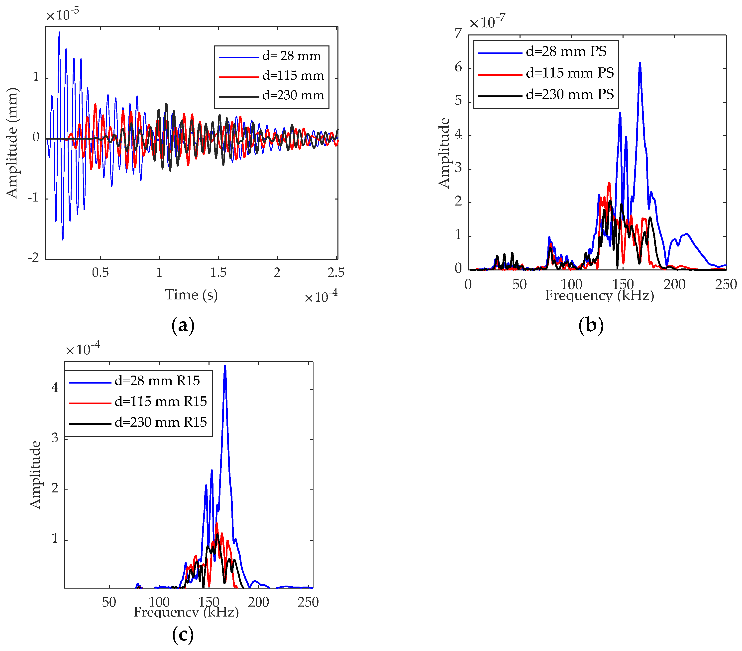
4.2. Virtual Perfect Sensor versus R15 Sensor for the Reference Sample: Characterization of the Reference Propagation Medium

The signals recorded in the undamaged α sample constituted the baseline. With the α sample, it was possible to obtain information on the influence of the wave propagation path on the received signal. Figure 6a shows the signals recorded by the perfect sensor at 28 mm, 115 mm and 230 mm from the transmitter, respectively. Figure 6b shows the corresponding fast Fourier transform. We can observe a significant decrease in the amplitude and in the frequency content due to the propagation effect. We note a decrease in the frequency content above 200 kHz with increasing propagation distance in the undamaged material. This effect is greatly modified by considering the sensor frequency sensitivity (Figure 6c). The detected frequencies are centered around 150 kHz. Frequencies below 100 kHz are suppressed, as well as those above 200 kHz. Therefore, the sensor conceals the difference in the frequency content due to the wave propagation in the assembly, such as, for instance, the frequency content above 200 kHz close to the emitting sensor or the frequency content below 50 kHz at a distance from it. The range of received frequencies actually corresponds to a frequency range in which the sensor is very sensitive and resonant (Figure 3).

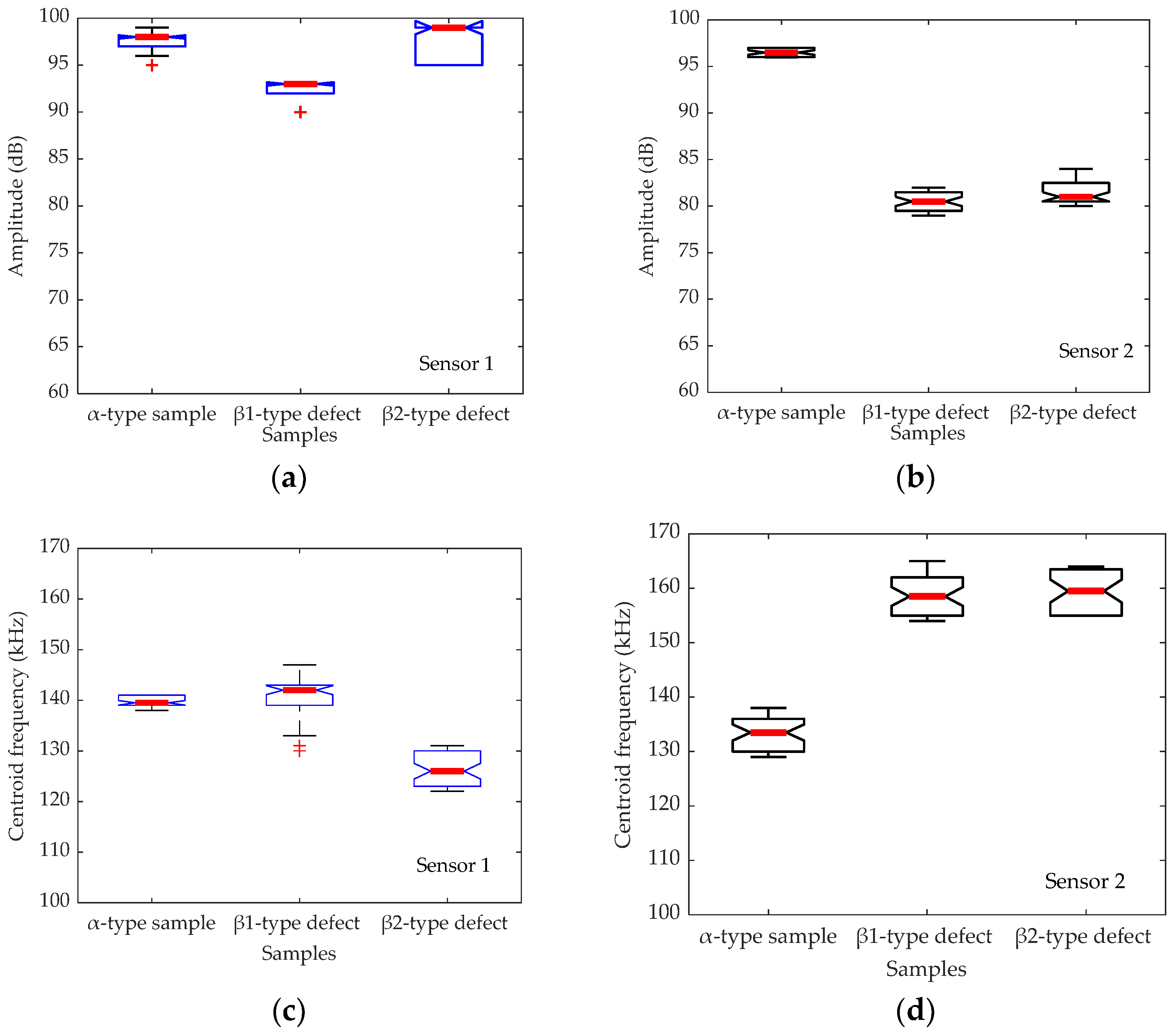
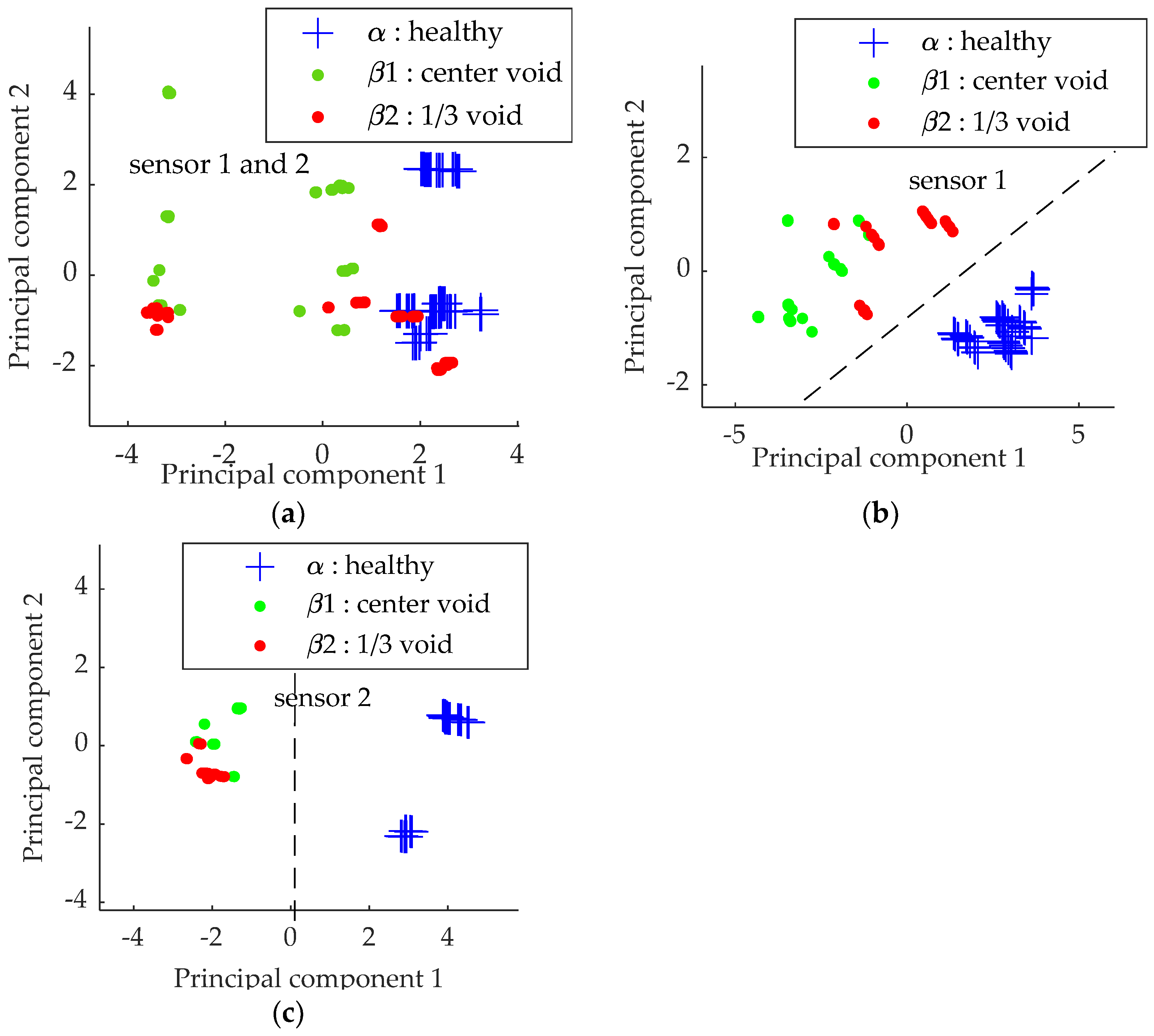
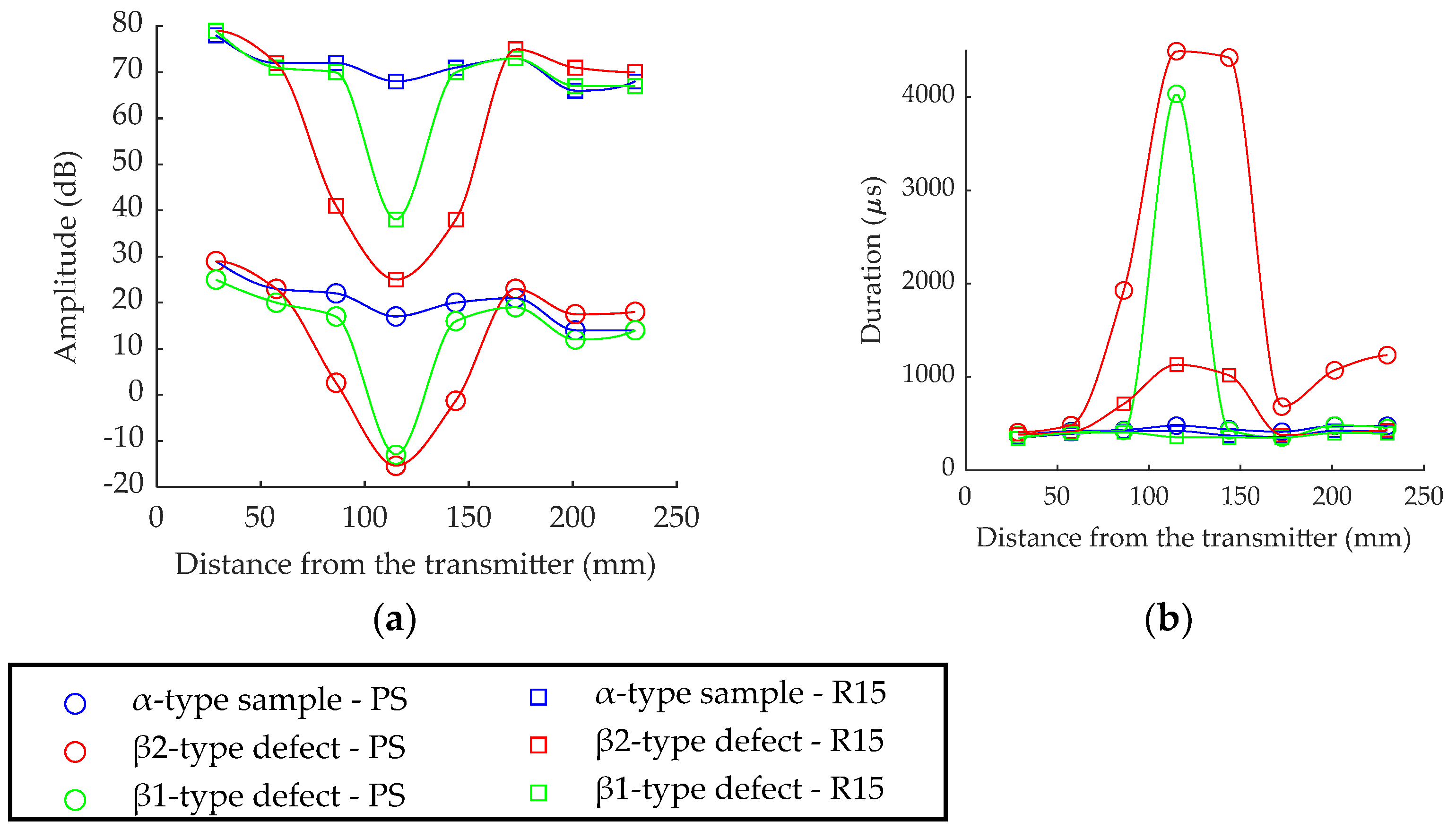
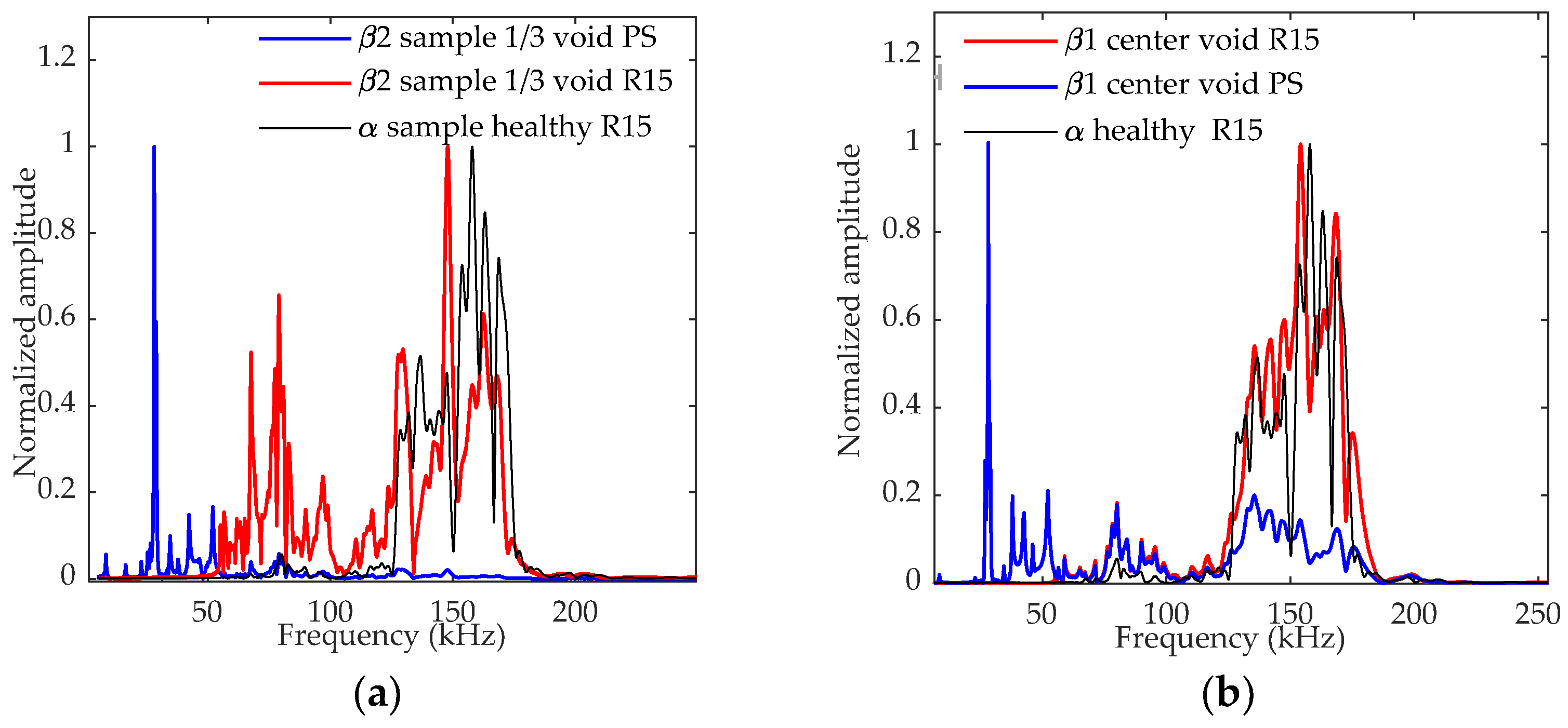
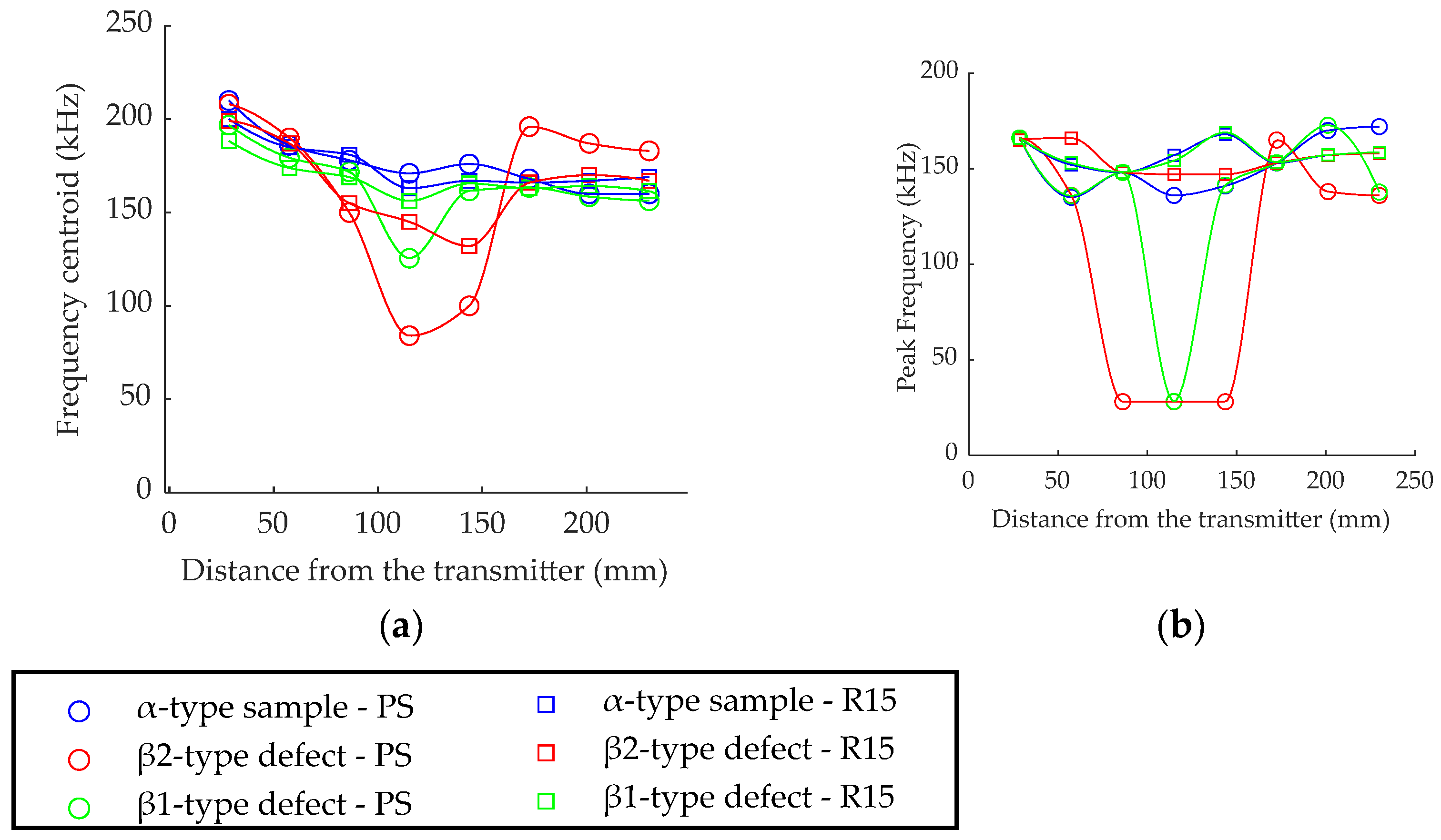
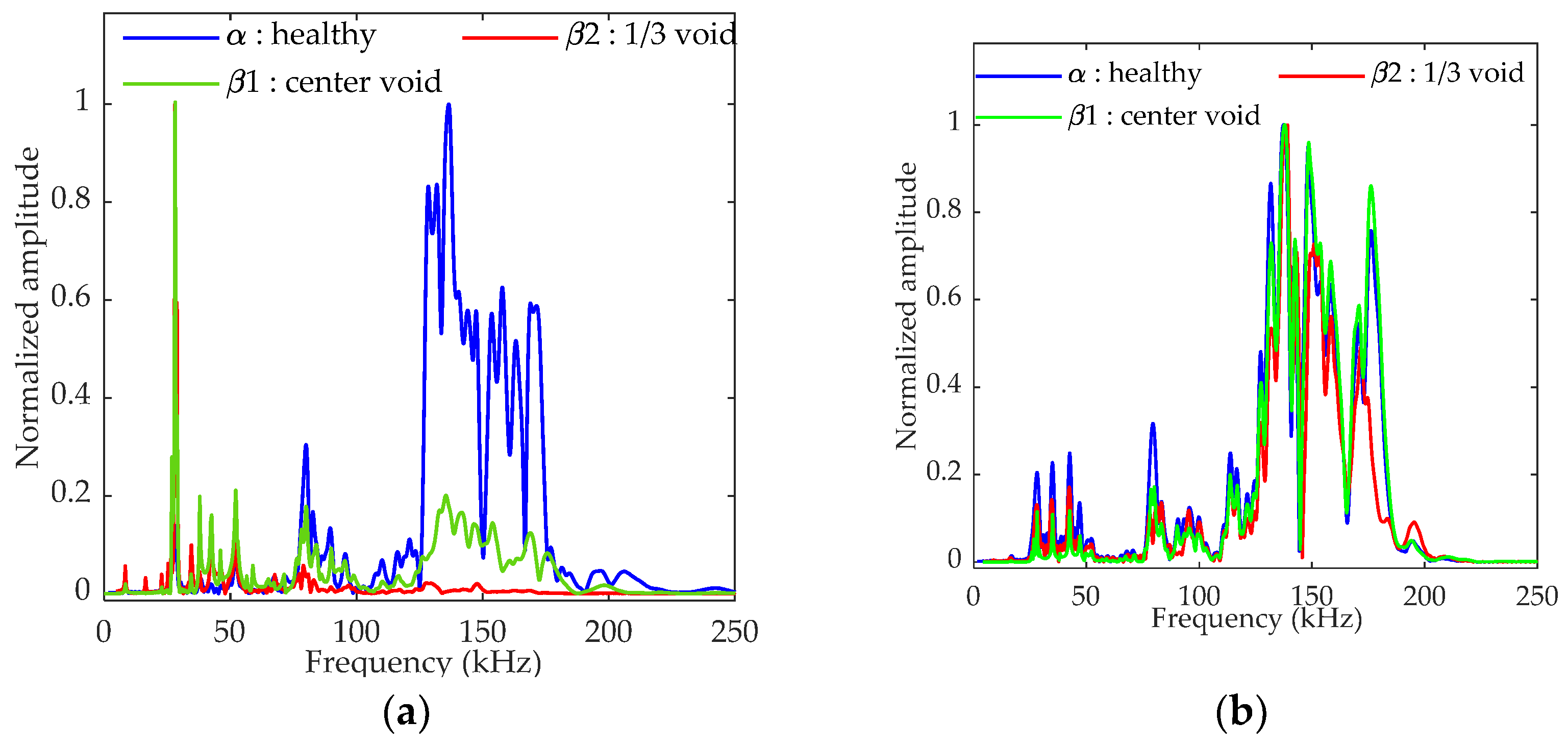
4.3. Influence of the Voids on AE Parameters

Figure 7 shows the variation of two descriptors (amplitude and duration) evaluated in the time domain as a function of the distance between the transmitter (T) and the receiver. The data collected by the perfect sensor or obtained by the R15 sensor are shown for the reference assembly and for the β samples. For the perfect sensor, we can observe a significant decrease in the amplitude at the epicenter of the defect, which is more evident for the void of larger size in β2. The signal duration increases significantly at the epicenter of the void. For all descriptors in time domain, the characteristics of the signals received after the void are significantly equivalent to those of the reference. The simulation with the perfect sensor highlights the difficulty of detecting the defect for a sensor not located at the epicenter of the void with the conventional parameters extracted in AE in the time domain. In contrast, it highlights the effect of the void size on the descriptors calculated at the defect epicenter.

Considering the actual R15 rather than the perfect sensor results in a similar variation in the amplitude as a function of the distance to the transmitter and considerably reduces the influence of the void on the signal duration. This is especially true for the smaller void, which no longer presents a significant difference from the reference material at the defect epicenter. Beyond the defect, the differences between the reference material and the material with defects are not marked or are even non-existent. This leads to the conclusion that using the R15 sensor significantly reduces the probability of detecting voids using time-domain descriptors.

The variation of the descriptors in the frequency domain as a function of the distance to the transmitter is shown in Figure 8. We can observe a significant decrease in the frequency content of the signal recorded with the perfect sensor just above the defect. The frequencies around 150 kHz are attenuated compared to lower frequencies. The reduction of the frequency content evolves with the size of the defect. Indeed, the centroid frequency is smaller than 100 kHz for the β2 defect and above 100 kHz for the smaller defect in β1. The peak frequency is also modified, but not affected by the size of the defect.

It was found that the defect size has an influence on the signature of the AU signal recorded by sensor 2 and could be discriminated with the perfect sensor or in applications with wideband sensors that are not expected to modify the measured frequency range. Using the R15 sensor, a modification of the centroid frequency can be observed although the differences are much less marked. On the other hand, for the peak frequency, there is no difference compared to the reference configuration. Considering the actual R15 sensor also reduces the probability of detecting voids in the frequency domain in comparison with the perfect sensor. Figure 9a represents the fast Fourier transform (FFT) for the sensor 2 and sensor 1 signals, calculated for the reference sample and the β samples.

It appears that the magnitude of the frequency band at about 80–250 kHz decreased significantly with the void size, whereas the magnitude at about 50 kHz increased considerably at the epicenter of the defect. The data calculated with the perfect sample confirm a significant decrease in the frequency content above 100 kHz for sensor 2, with a magnitude depending on the defect size. Indeed, in the undamaged sample, 78% of the spectrum energy was in the 125–200 kHz frequency range, whereas it was only 53% for β1 and 17% for β2. The modification of this frequency content can be correlated with the void size. At the sensor 1 location, no significant differences were observed. Nevertheless, the R15 sensor amplified the frequency content around 150 kHz due to its resonance and eliminated this reduction in frequency content (Figure 10a,b) even for sensor 2. The energy contained in the 125–200 kHz frequency band was 91% and 87%, respectively, for the undamaged sample and the sample containing a β1-type defect. Separation from the undamaged material was therefore difficult, and the probability of detection decreased with the size of the void.

5. Conclusions

The location of the sensor with respect to a known defect location is crucial for defect detection using AU inspection. The time and frequency descriptors of the signals acquired by the receiver sensor are significantly influenced by the presence of a void, compared to an undamaged specimen, only if the receiver sensor is located on the assembly surface near the defect epicenter. It is not straightforward to highlight the void’s presence when the sensor is placed too far from the defect epicenter. The time (amplitude, energy) and frequency (centroid frequency, peak frequency) descriptors of the signals acquired with a perfect sensor were all more affected as the defect size increased. This effect was attenuated when considering an actual R15 sensor, especially for the smaller defect size. This result highlights the difficulty of using AE descriptors (parameters extracted from the recorded signals) that reduce the signal data to only a few parameters, some of which become irrelevant for defect detection when using an actual sensor with resonance in a specific frequency range.

Both the relative location of the sensor with respect to the defect epicenter and the type of receiver sensor are thus fundamental for defect detection using the AU method. The proposed model enables the parameters affected by the size of the defect (amplitude, centroid frequency, etc.) to be determined, and an analysis based on the relevant parameters increases the probability of detection of voids. For instance, a wideband sensor should be preferred for optimal void detection.

References

1. Chataigner, S.; Benzarti, K.; Foret, G.; Caron, J.F.; Gemignani, G.; Brugiolo, M.; Calderon, I.; Pinero, I.; Birtel, V.; Lehmann, F. Design and evaluation of an externally bonded CFRP reinforcement for the fatigue reinforcement of old steel structures. Eng. Struct. 2018, 177, 556–565. [Google Scholar] [CrossRef]
2. Lepretre, E.; Chataigner, S.; Dieng, L.; Gaillet, L. Fatigue strengthening of cracked steel plates with CFRP laminates in the case of old steel materials. Constr. Build. Mater. 2018, 174, 421–432. [Google Scholar] [CrossRef]
3. Alsayed, S.H.; Al-Salloum, Y.A.; Almusallam, T.H. Fibre-reinforced polymer repair material: Some facts. In Proceedings of the Institution of Civil Engineers—Civil Engineering; Thomas Telford Ltd.: London, UK, 2000; Volume 138, pp. 131–134. [Google Scholar]
4. Adams, R.D.; Cawley, P. A review of defect types and nondestructive testing techniques for composites and bonded joints. NDT Int. 1988, 21, 208–222. [Google Scholar]
5. Adams, R.D.; Drinkwater, B.W. Nondestructive testing of adhesively-bonded joints. Department of Mechanical Engineering. NDT E Int. 1997, 30, 93–98. [Google Scholar] [CrossRef]
6. Guyott, C.C.H.; Cawley, P.; Adams, R.D. The Non-destructive Testing of Adhesively Bonded Structure: A Review. J. Adhes. 1986, 20, 129–159. [Google Scholar] [CrossRef]
7. Nieminen, A.O.K.; Koenig, J.L. Macroscopic and modern microscopic NDE methods for adhesive bond structures. Int. J. Adhes. Adhes. 1991, 11, 5–10. [Google Scholar] [CrossRef]
8. Ribeiro, F.; Campilho, R.; Carbas, R.; da Silva, L. Strength and damage growth in composite bonded joints with defects. Compos. Part B Eng. 2016, 100, 91–100. [Google Scholar] [CrossRef]
9. Xu, W.; Wei, Y. Strength analysis of metallic bonded joints containing defects. Comput. Mater. Sci. 2012, 53, 444–450. [Google Scholar] [CrossRef] [Green Version]
10. Yilmaz, B.; Jasiuniene, E. Advanced ultrasonic NDT for weak bond detection in composite-adhesive bonded structures. Int. J. Adhes. Adhes. 2020, 102, 102675. [Google Scholar] [CrossRef]
11. Yilmaz, B.; Asokkumar, A.; Jasiuniene, E.; KažysAppl, R.J. Air-Coupled, Contact, and Immersion Ultrasonic Non-Destructive Testing: Comparison for Bonding Quality Evaluation. Appl. Sci. 2020, 10, 6757. [Google Scholar] [CrossRef]
12. Yang, S.; Gu, L.; Gibson, R.F. Nondestructive detection of weak joints in adhesively bonded composite structures. Compos. Struct. 2001, 51, 63–71. [Google Scholar] [CrossRef]
13. Palumbo, D.; Tamborrino, R.; Galietti, U.; Aversa, P.; Tatì, A.; Luprano, V. Ultrasonic analysis and lock-in thermography for debonding evaluation of composite adhesive joints. NDT E Int. 2016, 78, 1–9. [Google Scholar] [CrossRef]
14. Schroeder, J.A.; Ahmed, T.; Choudhry, B.; Shepard, S. Non destructive testing of structural composites and adhesively bonded composite joints: Pulsed thermography. Compos. Part A Appl. Sci. Manuf. 2002, 33, 1511–1517. [Google Scholar] [CrossRef]
15. Wang, R.; Wu, Q.; Xiong, K.; Zhang, H.; Okabe, Y. Evaluation of the matrix crack number in carbon fiber reinforced plastics using linear and nonlinear acousto-ultrasonic detections. Compos. Struct. 2021, 255, 112962. [Google Scholar] [CrossRef]
16. le Crom, B.; Castaings, M. Shear horizontal guided wave modes to infer the shear stiffness of adhesive bond layers. J. Acoust. Soc. Am. 2010, 127, 2220–2230. [Google Scholar] [CrossRef]
17. la Rocca, C.; Moysan, J.; Payan, C. Characterization of an epoxy bonded aluminum alloy sample applying dynamic acousto elastic testing. In AIP Conference Proceedings; American Institute of Physics: Melville, NY, USA, 2012; Volume 1430, pp. 1261–1267. [Google Scholar]
18. Vary, A.; Bowles, K.J. Use of an Acousto-ultrasonic technique for nondestructive evaluation of fiber composite strength. In Proceedings of the 33rd Annual Conference of the Society of the Plastics Industry, Washington, DC, USA, 7–10 February 1978. [Google Scholar]
19. Srivastava, V.K.; Prakash, R. Acousto-ultrasonic evaluation of the strength of composite material adhesive joints. In Acousto-Ultrasonics: Theory and Application; Springer Science Business Media, LLC: Boston, MA, USA, 1988; pp. S345–S353. [Google Scholar]
20. Srivastava, V.K. Acousto-ultrasonic evaluation of interface bond strength of coated glass fibre-reinforced epoxy resin composites. Compos. Struct. 1995, 30, 281–285. [Google Scholar] [CrossRef]
21. Tanary, S. Characterization of Adhesively Bonded Joints Using Acousto-Ultrasonics. Ph.D. Thesis, University of Ottawa, Ottawa, ON, Canada, 1988. [Google Scholar]
22. Tanary, S.; Haddad, M.; Fahr, A.; Lee, S. Nondestructive Evaluation of Adhesively Bonded Joints in Graphite/Epoxy Composites Using Acousto-Ultrasonics. J. Press. Vessel. Technol. 1992, 114, 344–352. [Google Scholar] [CrossRef]
23. Kwon, O.Y.; Lee, S.H. Acousto-ultrasonic evaluation of adhesively bonded CFRP-aluminum joints. NDT E Int. 1999, 32, 153–160. [Google Scholar] [CrossRef]
24. Sarr, C.A.T.; Chataigner, S.; Gaillet, L.; Godin, N. Nondestructive evaluation of FRP-reinforced structures bonded joints using acousto-ultrasonic: Towards diagnostic of damage state. Constr. Build. Mater. 2021, 313, 125499. [Google Scholar] [CrossRef]
25. Barile, C.; Casavola, C.; Pappalettera, G.; Vimalathithan, P.K. Acousto-ultrasonic evaluation of interlaminar strength on CFRP laminates. Compos. Struct. 2019, 208, 796–805. [Google Scholar] [CrossRef]
26. Barile, C.; Casavola, C.; Pappalettera, G.; Pappalettere, C.; Vimalathithan, P.K. Detection of Damage in CFRP by Wavelet Packet Transform and Empirical Mode Decomposition: An Hybrid Approach. Appl. Compos. Mater. 2020, 27, 641–655. [Google Scholar] [CrossRef]
27. Janapati, V.; Kopsaftopoulos, F.; Li, F.; Lee, S.J.; Chang, F.-K. Damage Detection Sensitivity Characterization of Acousto-Ultrasound-based SHM Techniques. Struct. Health Monit. 2016, 15, 143–161. [Google Scholar] [CrossRef]
28. Matt, H.; Bartoli, I.; di Scalea, F.L. Ultrasonic guided wave monitoring of composite wing skin-to-spar bonded joints in aerospace structures. J. Acoust. Soc. Am. 2005, 118, 2240–2252. [Google Scholar] [CrossRef]
29. Lowe, M.J.S.; Challis, R.E.; Chan, C.W. The transmission of Lamb waves across adhesively bonded lap joints. J. Acoust. Soc. Am. 2000, 107, 1333–1345. [Google Scholar] [CrossRef] [PubMed]
30. Hanneman, S.E.; Kinra, V.K. A new technique for ultrasonic non-destructive evaluation of adhesive joints: Part I. Theory. Exp. Mech. 1992, 32, 323–331. [Google Scholar] [CrossRef]
31. Di Scalea, F.L.; Rizzo, P.; Marzani, A. Propagation of ultrasonic guided waves in lap-shear adhesive joints: Case of incident A0 lamb wave. J. Acoust. Soc. Am. 2003, 115, 146–156. [Google Scholar] [CrossRef]
32. Koreck, J.; Valle, C.; Qu, J.; Jacobs, L.J. Computational characterization of adhesive bond properties using guided waves in bonded plates. J. Nondestruct. Eval. 2007, 26, 97–105. [Google Scholar] [CrossRef]
33. Vaziri, A.; Nayeb-Hashemi, H.; Hamidzadeh, H.R. Experimental and analytical investigations of the dynamic response of adhesively bonded single lap joints. J. Vib. Acoust. 2004, 126, 84–91. [Google Scholar] [CrossRef]
34. Sause, M.G.R.; Richler, S. Finite Element Modelling of Cracks as Acoustic Emission Sources. J. Nondestruct. Eval. 2015, 34, 4. [Google Scholar] [CrossRef] [Green Version]
35. Sause, M.G.R.; Horn, S. Simulation of Acoustic Emission in Planar Carbon Fiber Reinforced Plastic Specimens. J. Nondestruct. Eval. 2010, 29, 123–142. [Google Scholar] [CrossRef]
36. Zelenyak, A.-M.; Schorer, N.; Sause, M.G. Modeling of ultrasonic wave propagation in composite laminates with realistic discontinuity representation. Ultrasonics 2018, 83, 103–113. [Google Scholar] [CrossRef] [PubMed]
37. Zhang, L.; Yalcinkaya, H.; Ozevin, D. Numerical approach to absolute calibration of piezoelectric acoustic emission sensors using multiphysics simulations. Sens. Actuators A Phys. 2017, 256, 12–23. [Google Scholar] [CrossRef] [Green Version]
38. Wu, B.S.; McLaskey, G.C. Broadband Calibration of Acoustic Emission and Ultrasonic Sensors from Generalized Ray Theory and Finite Element Models. J. Nondestruct. Eval. 2018, 37, 8. [Google Scholar] [CrossRef]
39. Sause, M.G.; Hamstad, M.A. Numerical modeling of existing acoustic emission sensor absolute calibration approaches. Sens. Actuators A Phys. 2018, 269, 294–307. [Google Scholar] [CrossRef]
40. Hamam, Z.; Godin, N.; Fusco, C.; Monnier, T. Modelling of Acoustic Emission Signals Due to Fiber Break in a Model Composite Carbon/Epoxy: Experimental Validation and Parametric Study. Appl. Sci. 2019, 9, 5124. [Google Scholar] [CrossRef] [Green Version]
41. Le Gall, T.; Monnier, T.; Fusco, C.; Godin, N.; Hebaz, S.-E. Towards Quantitative Acoustic Emission by Finite Element Modelling: Contribution of Modal Analysis and Identification of Pertinent Descriptors. Appl. Sci. 2018, 8, 2557. [Google Scholar] [CrossRef] [Green Version]
42. Hamam, Z.; Godin, N.; Reynaud, P.; Fusco, C.; Carrère, N.; Doitrand, A. Transverse cracking induced acoustic emission in carbon fiber-epoxy matrix composite laminates. Materials 2022, 15, 394. [Google Scholar] [CrossRef]
43. Hamam, Z.; Godin, N.; Fusco, C.; Doitrand, A.; Monnier, T. Acoustic Emission Signal Due to Fiber Break and Fiber Matrix Debonding in Model Composite: A Computational Study. Appl. Sci. 2021, 11, 8406. [Google Scholar] [CrossRef]
44. Dia, S.; Monnier, T.; Godin, N.; Zhang, F. Primary Calibration of Acoustic Emission Sensors by the Method of Reciprocity, Theoretical and Experimental Considerations. J. Acoust. Emiss. 2012, 30, 152–166. [Google Scholar]
45. Morizet, N.; Godin, N.; Tang, J.; Maillet, E.; Fregonese, M.; Normand, B. Classification of acoustic emission signals using wavelets and Random Forests: Application to localized corrosion. Mech. Syst. Signals Process. 2019, 70–71, 1026–1037. [Google Scholar] [CrossRef]
Figure 1. Schematic representation of the composite/metal assemblies: (a) α-type sample; (b) sample with β2-type defect (1/3 void); (c) sample with β1-type defect (centered void).
Applsci 12 04153 g001
Figure 2. (a) Schematic representation of the composite/metal assemblies with the location of the defect and sensors (transmitter, sensor 2 and sensor 1 denote the positions of the transmitter and receivers during the tests). (b) Simulation of the AU test indicating the locations of the virtual transmitter and receiver sensors (T denotes transmitter), where each virtual receiver is separated by about 28 mm.
Applsci 12 04153 g002
Figure 3. (a) Aperture function for the R15 sensors: evolution of the k factor versus the distance from the center of the sensor surface r. (b) Reception response of the R15 sensor obtained with the reciprocity method on a steel block.
Applsci 12 04153 g003
Figure 4. Experimental results. Amplitude (a,b) and centroid frequency (c,d) recorded by sensor 1 (a,d) and sensor 2 (b,c). (The “+” symbol indicates outliers).
Applsci 12 04153 g004
Figure 5. First principal component as a function of second principal component for α, β1 and β2 samples obtained with: (a) sensor 1 and 2 data; (b) sensor 1 data only; (c) sensor 2 data only.
Applsci 12 04153 g005
Figure 6. Simulated signal without AE sensor effect in (a) time domain and (b) frequency domain. (c) Fast Fourier transform (FFT) of the simulated signals recorded by the R15 sensor.
Applsci 12 04153 g006
Figure 7. Variation of (a) amplitude and (b) duration as a function of the distance between the transmitter and the perfect sensor (PS, o) or the R15 sensor (□) for the various assemblies.
Applsci 12 04153 g007
Figure 8. Variation of (a) frequency centroid and (b) peak frequency versus the distance between the emitter and the perfect sensor (PS, o) or R15 sensor (□) for the various assemblies.
Applsci 12 04153 g008
Figure 9. FFT of the simulated signals recorded by the perfect sensor (PS): (a) sensor location 2; (b) sensor location 1.
Applsci 12 04153 g009
Figure 10. FFT of the simulated signals recorded by the R15 sensor or by the perfect sensor (PS), at sensor location 2: (a) for the β2 sample; (b) for the β1 sample. The curve obtained for the α sample is also superimposed.
Applsci 12 04153 g010