
SOH Estimation of Li-Ion Battery Using Discrete Wavelet Transform and Long Short-Term Memory Neural Network


Abstract
:1. Introduction
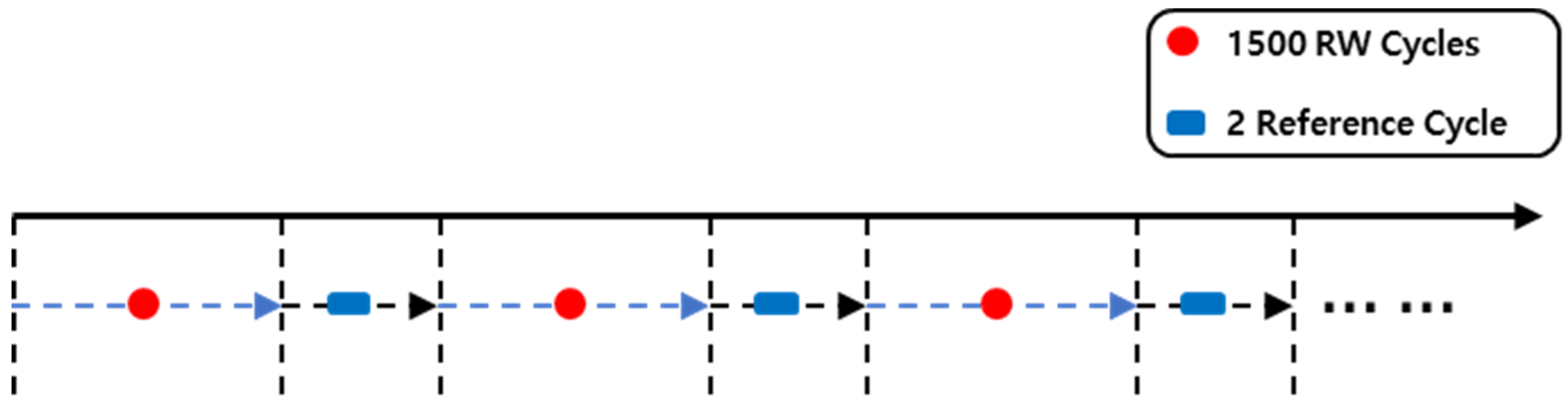
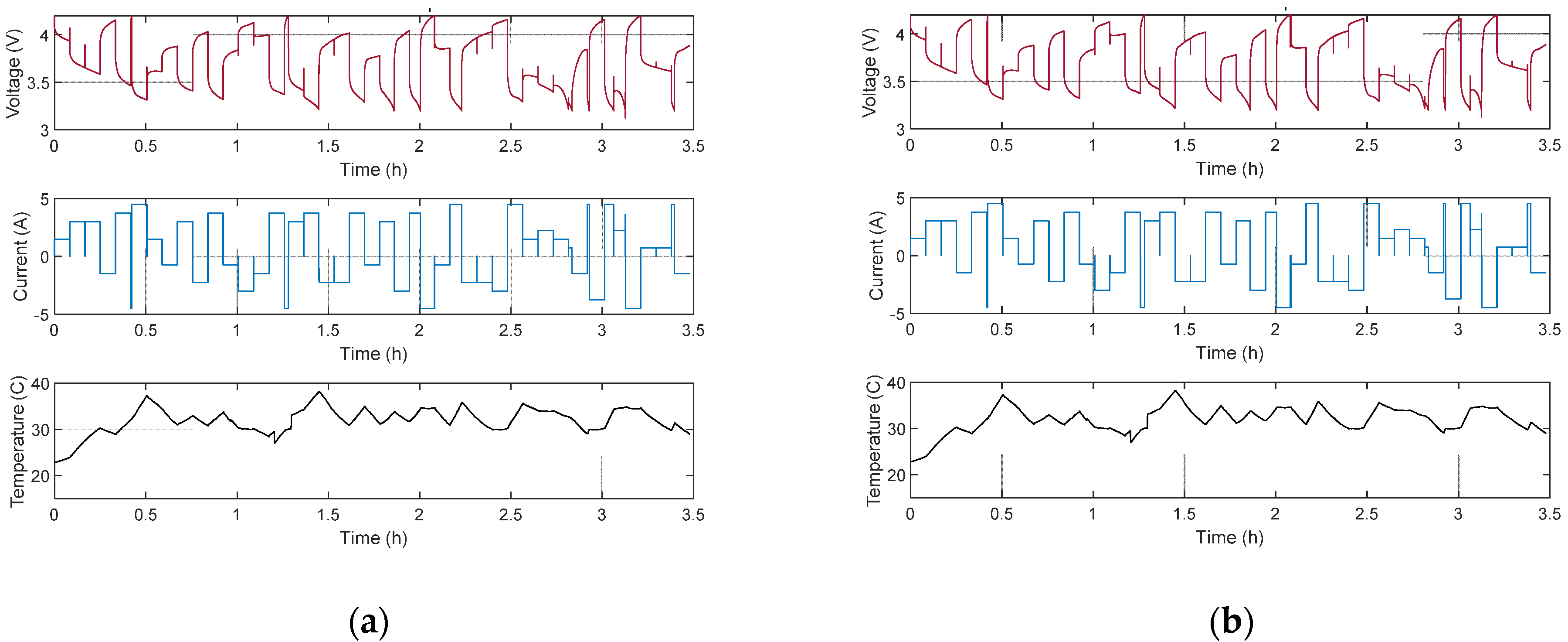
2. Data Composition
3. SOH Estimation Methods
3.1. Preprocessing Methods
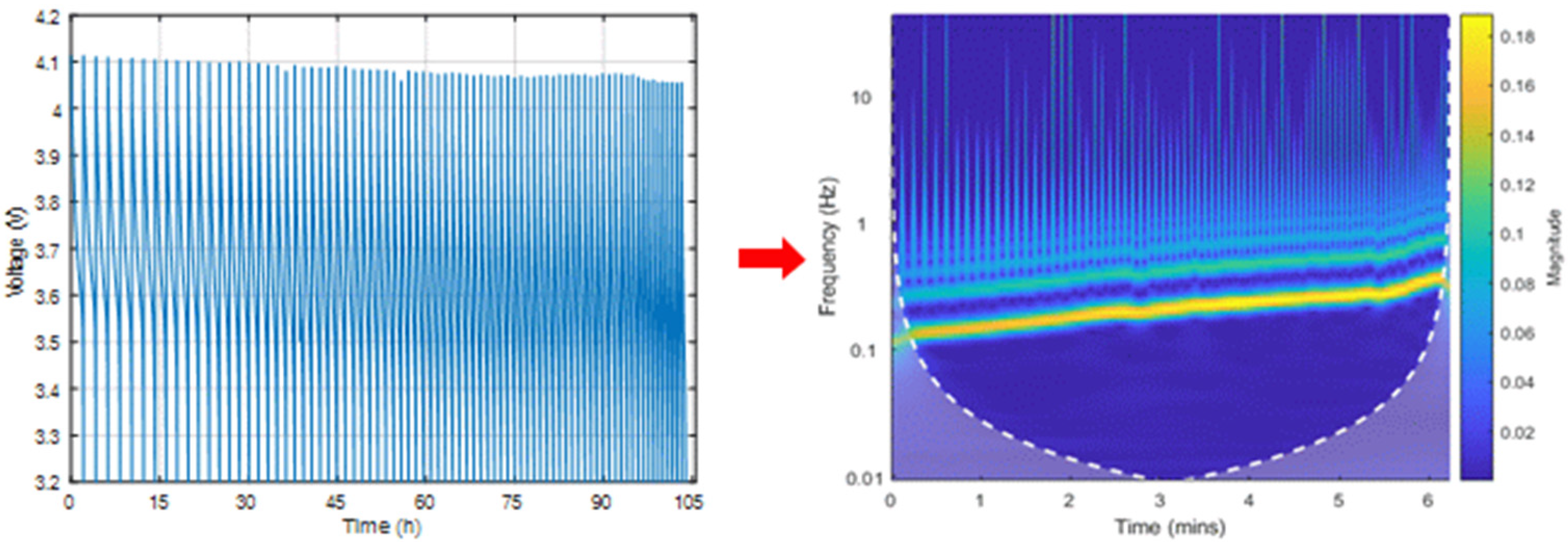
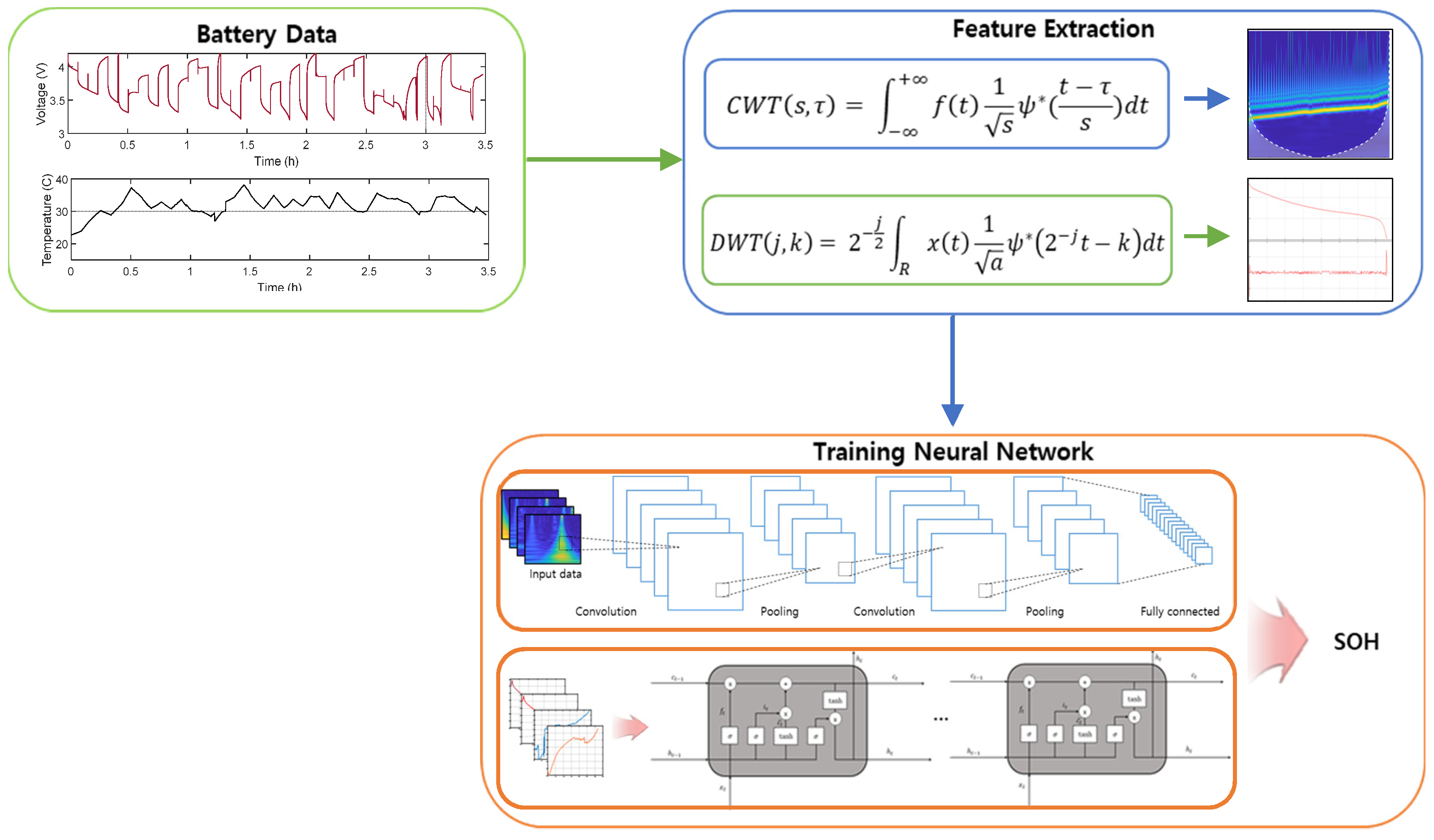
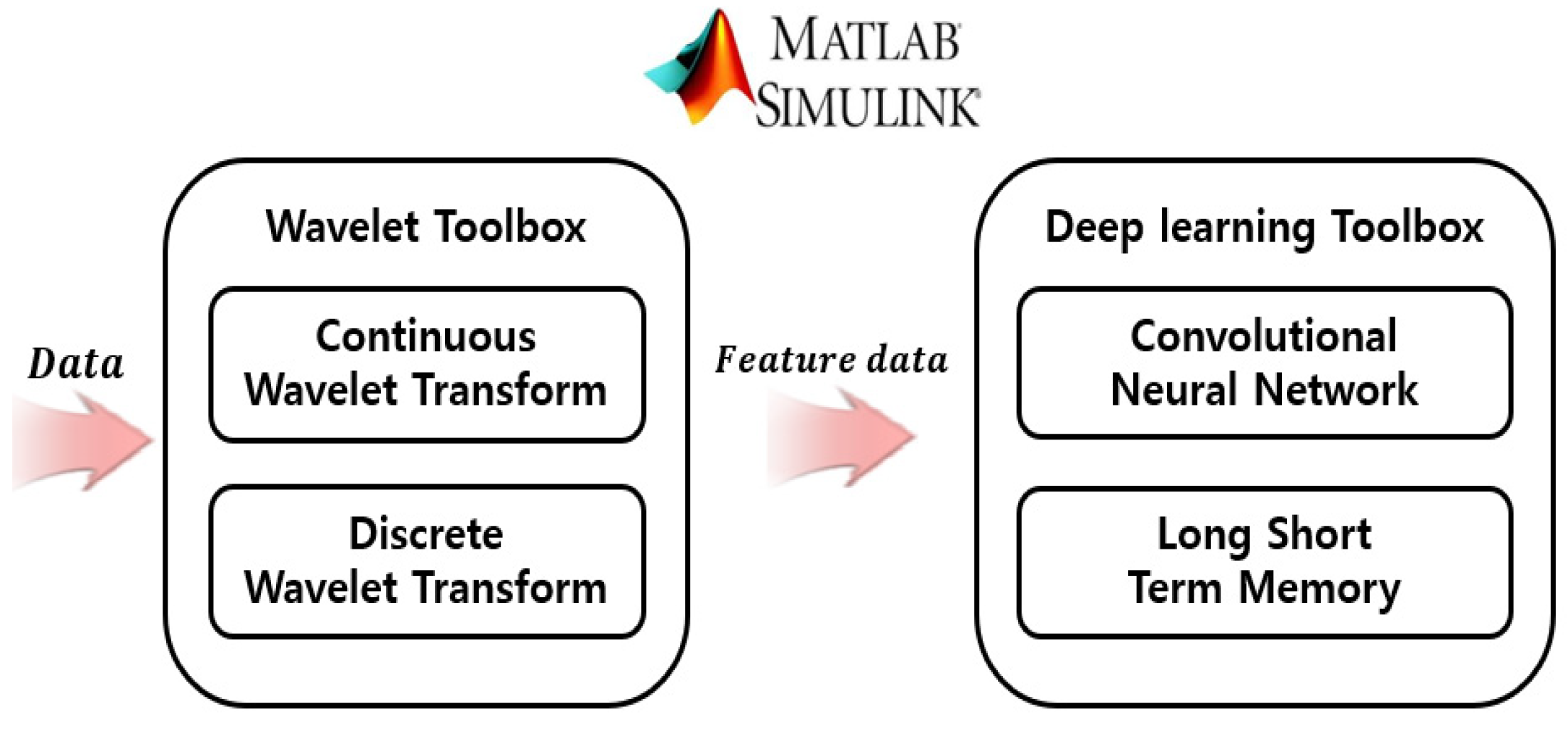
3.1.1. Continuous Wavelet Transform (CWT)
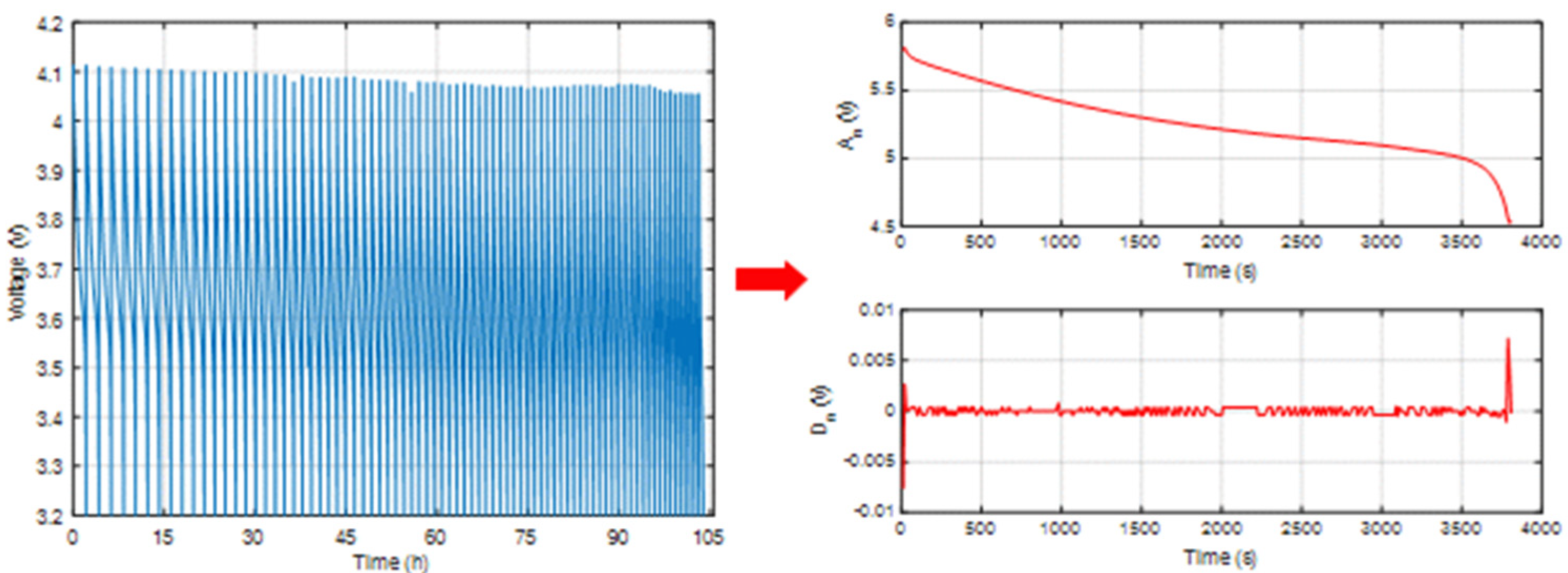
3.1.2. Discrete Wavelet Transform (DWT)
3.2. Deep Learning Methods
3.2.1. Convolutional Neural Network (CNN)
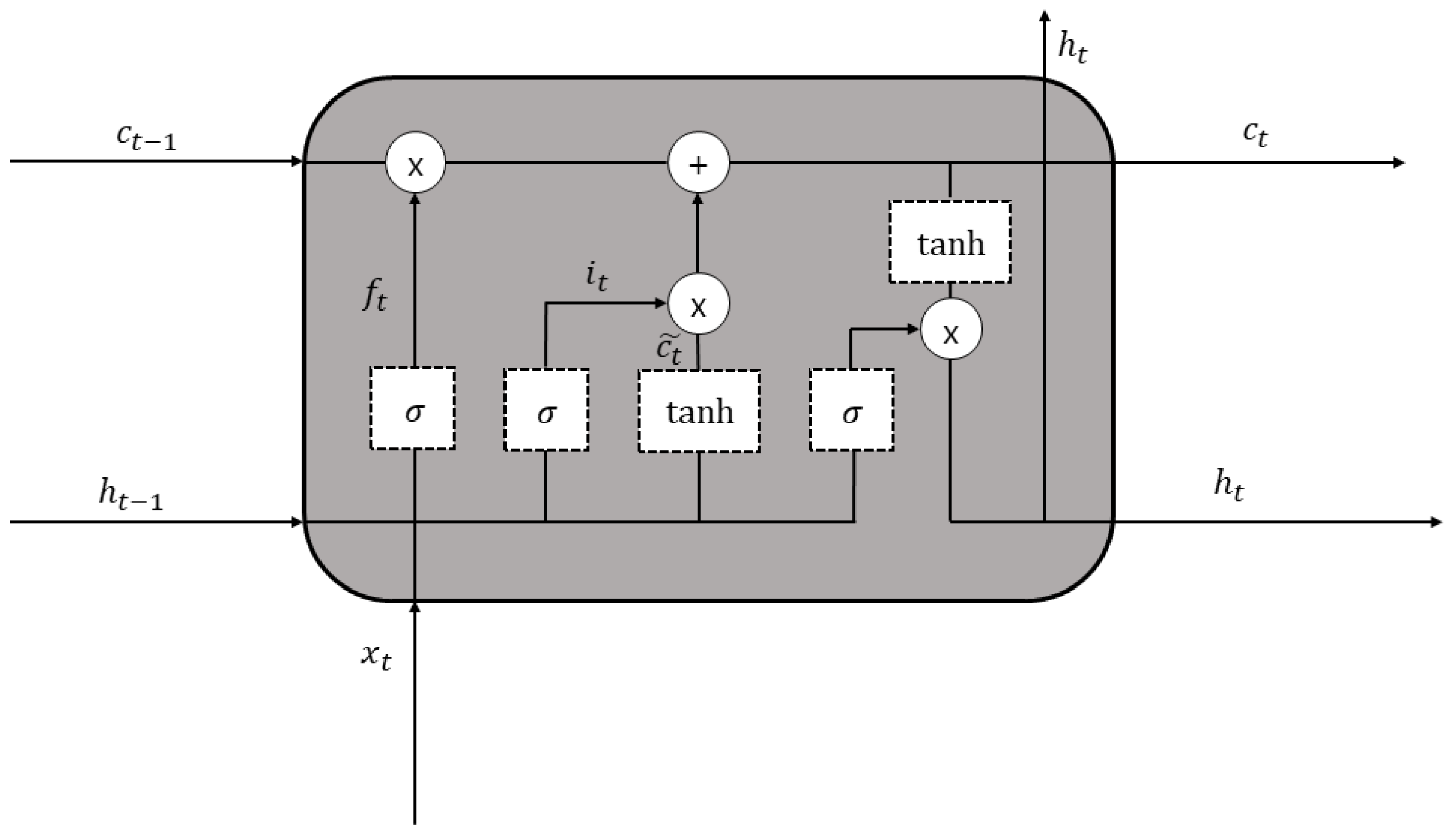
3.2.2. Long Short-Term Memory (LSTM)
3.2.3. Construction of a Neural Network Model
4. Simulation
4.1. Learning Using Data
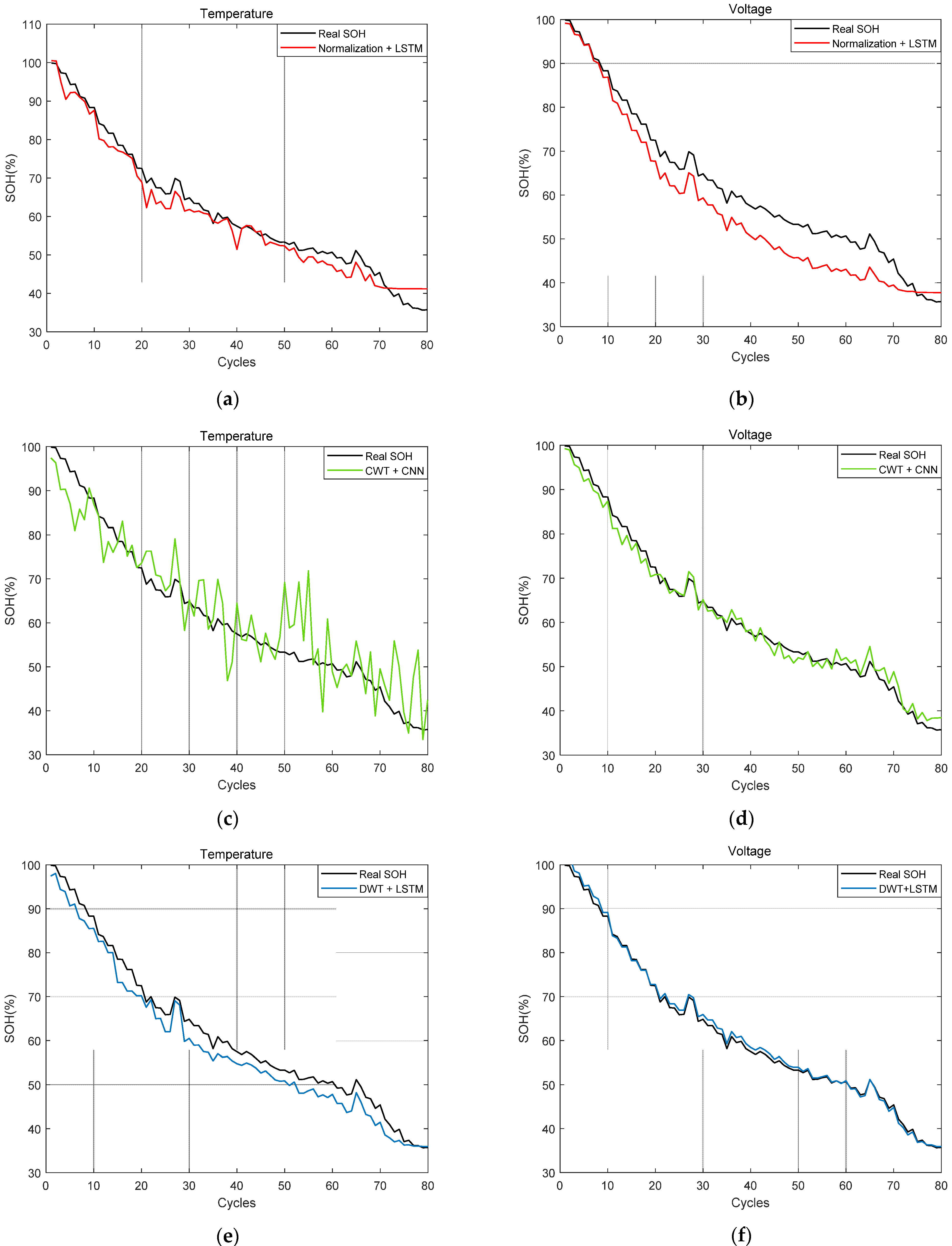
4.2. Comparison of Model Performances Using the Battery Dataset
5. Conclusions
Author Contributions
Funding
Conflicts of Interest
References
- Cano, Z.P.; Banham, D.; Ye, S.; Hintennach, A.; Lu, J.; Fowler, M.; Chen, Z. Batteries and fuel cells for emerging electric vehicle markets. Nat. Energy 2018, 3, 279–289. [Google Scholar] [CrossRef]
- Nishi, Y. Lithium ion secondary batteries; Past 10 years and the future. J. Power Sources 2001, 100, 101–106. [Google Scholar] [CrossRef]
- Abada, S.; Marlair, G.; Lecocq, A.; Petit, M.; Sauvant-Moynot, V.; Huet, F. Safety focused modeling of lithium-ion batteries: A review. J. Power Sources 2016, 306, 178–192. [Google Scholar] [CrossRef]
- Sun, J.; Li, J.; Zhou, T.; Yang, K.; Wei, S.; Tang, N.; Dang, N.; Li, H.; Qiu, X.; Chen, L. Toxicity, a serious concern of thermal runaway from commercial Li-ion battery. Nano Energy 2016, 27, 313–319. [Google Scholar] [CrossRef]
- Wang, Y.; Zhang, C.; Chen, Z. An adaptive remaining energy prediction approach for lithium-ion batteries in electric vehicles. J. Power Sources 2016, 305, 80–88. [Google Scholar] [CrossRef]
- Wang, Y.; Zhang, C.; Chen, Z. A method for joint estimation of state-of-charge and available energy of LiFePO4 batteries. Appl. Energy 2014, 135, 81–87. [Google Scholar] [CrossRef]
- Feng, X.; Lu, L.; Ouyang, M.; Li, J.; He, X. A 3D thermal runaway propagation model for a large format lithium ion battery module. Energy 2016, 115, 194–208. [Google Scholar] [CrossRef]
- Waag, W.; Fleischer, C.; Sauer, D.U. Critical review of the methods for monitoring of lithium-ion batteries in electric and hybrid vehicles. J. Power Sources 2014, 258, 321–339. [Google Scholar] [CrossRef]
- Berecibar, M.; Garmendia, M.; Gandiaga, I.; Crego, J.; Villarreal, I. State of health estimation algorithm of LiFePO4 battery packs based on differential voltage curves for battery management system application. Energy 2016, 103, 784–796. [Google Scholar] [CrossRef]
- Dai, H.; Zhao, G.; Lin, M.; Wu, J.; Zheng, G. A novel estimation method for the state of health of lithium-ion battery using prior knowledge-based neural network and markov chain. IEEE Trans. Ind. Electron. 2019, 66, 7706–7716. [Google Scholar] [CrossRef]
- Stroe, D.I.; Swierczynski, M.; Stan, A.I.; Teodorescu, R.; Andreasen, S.J. Accelerated lifetime testing methodology for lifetime estimation of lithium-ion batteries used in augmented wind power plants. IEEE Trans. Ind. Appl. 2014, 50, 4006–4017. [Google Scholar] [CrossRef]
- Khumprom, P.; Yodo, N. A data-driven predictive prognostic model for lithium-ion batteries based on a deep learning algorithm. Energies 2019, 12, 660. [Google Scholar] [CrossRef] [Green Version]
- Kang, S.H.; Noh, T.W.; Lee, B.K. Machine Learning-based SOH Estimation Algorithm Using a Linear Regression Analysis. Trans. Korean Inst. Power Electron. 2021, 26, 241–248. [Google Scholar]
- Plett, G.L. Extended Kalman filtering for battery management systems of LiPB-based HEV battery packs—Part 1. Background. J. Power Sources 2004, 134, 252–261. [Google Scholar] [CrossRef]
- Kim, Y.; Bang, H. Introduction to Kalman Filter and Its Applications. Introd. Implement. Kalman Filter 2019, 1, 1–16. [Google Scholar] [CrossRef] [Green Version]
- Sepasi, S.; Ghorbani, R.; Liaw, B.Y. Inline state of health estimation of lithium-ion batteries using state of charge calculation. J. Power Sources 2015, 299, 246–254. [Google Scholar] [CrossRef]
- Chen, Z.P.; Wang, Q.T. The Application of UKF Algorithm for 18650-type Lithium Battery SOH Estimation. Appl. Mech. Mater. 2014, 519–520, 1079–1084. [Google Scholar] [CrossRef]
- Liang, J.; Peng, X.-Y. Improved particle filter for nonlinear system state. Electron. Lett. 2008, 44, 1275–1277. [Google Scholar] [CrossRef]
- Miao, Q.; Xie, L.; Cui, H.; Liang, W.; Pecht, M. Remaining useful life prediction of lithium-ion battery with unscented particle filter technique. Microelectron. Reliab. 2013, 53, 805–810. [Google Scholar] [CrossRef]
- Liu, D.; Yin, X.; Song, Y.; Liu, W.; Peng, Y. An on-line state of health estimation of lithium-ion battery using unscented particle filter. IEEE Access 2018, 6, 40990–41001. [Google Scholar] [CrossRef]
- Qu, J.; Liu, F.; Ma, Y.; Fan, J. A Neural-Network-Based Method for RUL Prediction and SOH Monitoring of Lithium-Ion Battery. IEEE Access 2019, 7, 87178–87191. [Google Scholar] [CrossRef]
- Oji, T.; Zhou, Y.; Ci, S.; Kang, F.; Chen, X.; Liu, X. Data-Driven Methods for Battery SOH Estimation: Survey and a Critical Analysis. IEEE Access 2021, 9, 126903–126916. [Google Scholar] [CrossRef]
- Nuhic, A.; Terzimehic, T.; Soczka-Guth, T.; Buchholz, M.; Dietmayer, K. Health diagnosis and remaining useful life prognostics of lithium-ion batteries using data-driven methods. J. Power Sources 2013, 239, 680–688. [Google Scholar] [CrossRef]
- Liu, D.; Zhou, J.; Liao, H.; Peng, Y.; Peng, X. A health indicator extraction and optimization framework for lithium-ion battery degradation modeling and prognostics. IEEE Trans. Syst. Man Cybern. Syst. 2015, 45, 915–928. [Google Scholar] [CrossRef]
- Li, Y.; Zhong, S.; Zhong, Q.; Shi, K. Lithium-ion battery state of health monitoring based on ensemble learning. IEEE Access 2019, 7, 8754–8762. [Google Scholar] [CrossRef]
- Ren, L.; Zhao, L.; Hong, S.; Zhao, S.; Wang, H.; Zhang, L. Remaining Useful Life Prediction for Lithium-Ion Battery: A Deep Learning Approach. IEEE Access 2018, 6, 50587–50598. [Google Scholar] [CrossRef]
- You, G.W.; Park, S.; Oh, D. Diagnosis of Electric Vehicle Batteries Using Recurrent Neural Networks. IEEE Trans. Ind. Electron. 2017, 64, 4885–4893. [Google Scholar] [CrossRef]
- El-Dalahmeh, M.; Al-Greer, M.; El-Dalahmeh, M.; Short, M. Time-frequency image analysis and transfer learning for capacity prediction of lithium-ion batteries. Energies 2020, 13, 5447. [Google Scholar] [CrossRef]
- Xu, J.; Mei, X.; Wang, X.; Fu, Y.; Zhao, Y.; Wang, J. A Relative State of Health Estimation Method Based on Wavelet Analysis for Lithium-Ion Battery Cell Cells. IEEE Trans. Ind. Electron. 2021, 68, 6973–6981. [Google Scholar] [CrossRef]
- Bole, B.; Kulkarni, C.; Daigle, M. Randomized battery usage data set. In NASA AMES Prognostics Data Repository; NASA Ames Research Center: Moffett Field, CA, USA, 2014. [Google Scholar]
- Gamero, L.G.; Vila, J.; Palacios, F. Wavelet transform analysis of heart rate variability during mycardial ischaemia. Med. Biol. Eng. Comput. 2002, 40, 72–78. [Google Scholar] [CrossRef]
- Li, X.; Zhang, W.; Ding, Q. Deep learning-based remaining useful life estimation of bearings using multi-scale feature extraction. Reliab. Eng. Syst. Saf. 2019, 182, 208–218. [Google Scholar] [CrossRef]
- Hochreiter, S.; Schmidhuber, J. Long short-term memory. Neural Comput. 1997, 9, 1735–1780. [Google Scholar] [CrossRef] [PubMed]
- Srivastava, N.; Hinton, G.; Krizhevsky, A.; Sutskever, I.; Salakhutdinov, R. Dropout: A simple way to prevent neural networks from overfitting. J. Mach. Learn. Res. 2014, 15, 1929–1958. [Google Scholar]


| Battery Properties | 18,650 LIBs |
| Manufacture | LG Chem |
| Chemistry | 18,650 lithium cobalt oxide vs. graphite |
| Nominal capacity | 2.10 Ah |
| Capacity range | 2.10~0.80 Ah |
| Voltage range | 4.2~3.2 V |
| Layer | Kernel Size | Kernel Number |
|---|---|---|
| Input Layer | N/A | - |
| Convolutional Layer 1 | 3 × 3 | 8 |
| Max Pooling Layer 1 | 2 × 2 | - |
| Convolutional Layer 2 | 3 × 3 | 16 |
| Max Pooling Layer 2 | 2 × 2 | - |
| Convolutional Layer 3 | 3 × 3 | 16 |
| Max Pooling Layer 3 | 2 × 2 | - |
| Convolutional Layer 4 | 3 × 3 | 16 |
| Max Pooling Layer 4 | 2 × 2 | - |
| Fully Connected Layer | N/A | 1 |
| Output Layer | N/A | - |
| Layer | Number |
|---|---|
| Input Layer | 2 |
| LSTM | 125 |
| Fully Connected Layer | 1 |
| Output Layer | 1 |
| Datasets | Method | Accuracy (%) | RMS (%) | MAE (%) | MAX (%) |
|---|---|---|---|---|---|
| Temperature | Normalization + LSTM | 93.49 | 6.51 | 4.13 | 17.39 |
| CWT + CNN | 94.38 | 5.61 | 4.11 | 20.22 | |
| DWT + LSTM | 96.45 | 3.55 | 3.36 | 6.03 | |
| Voltage | Normalization + LSTM | 94.85 | 5.15 | 4.58 | 7.84 |
| CWT + CNN | 97.71 | 2.29 | 1.80 | 4.98 | |
| DWT + LSTM | 98.92 | 1.07 | 0.91 | 2.57 |
| Indicator | Definitions |
|---|---|
| Maximum | The smallest data larger than median (Interquartile range) |
| Third quartile | The middle value between the median and the highest value of the dataset |
| Median | The middle value of the dataset |
| First quartile | The middle value between the median and the highest value of the dataset |
| Minimum | The highest value larger than median |
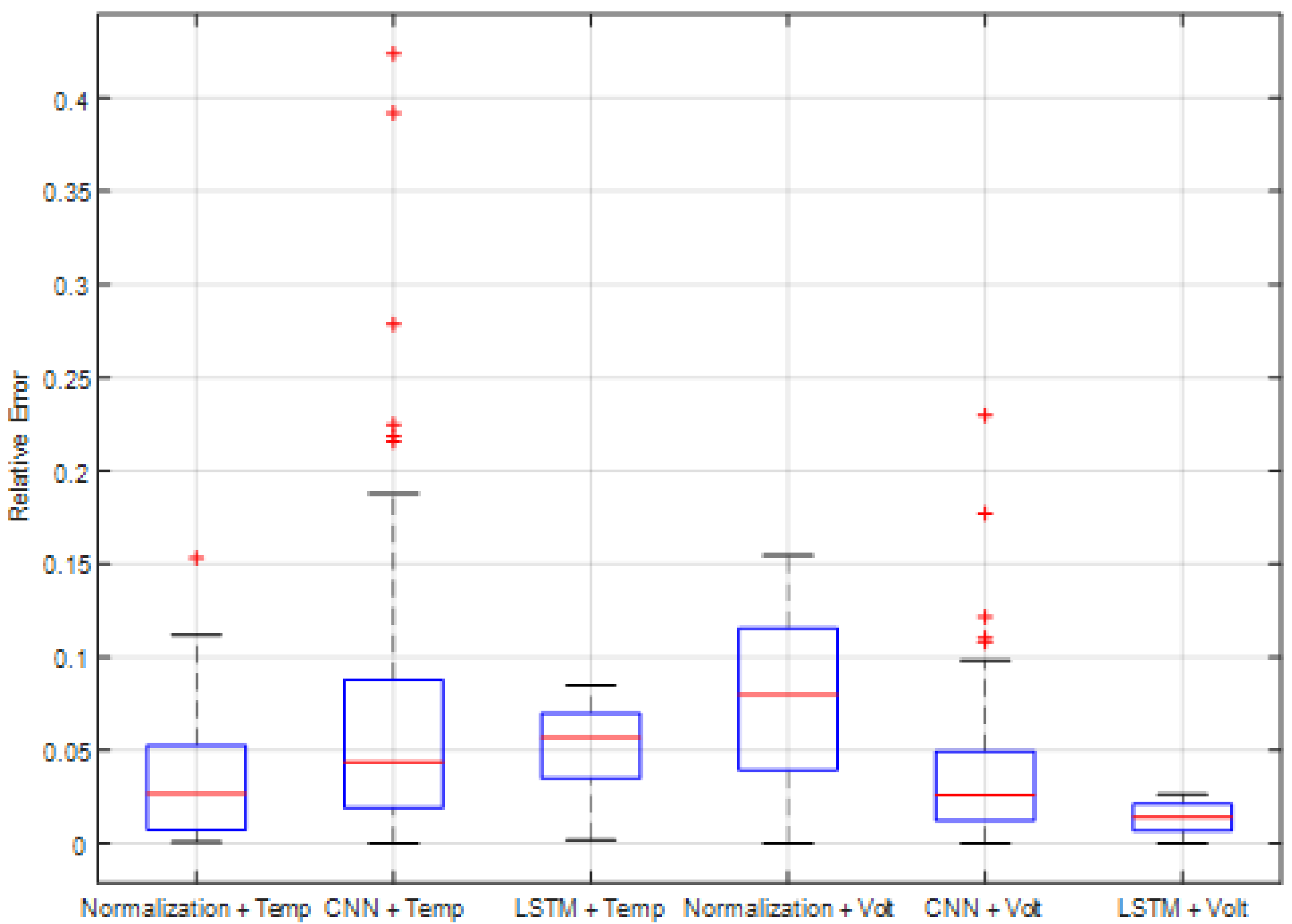
| Methods | Datasets | Maximum | Third Quartile | Median | First Quartile | Maximum | Outlier |
|---|---|---|---|---|---|---|---|
| Normalization + LSTM | Voltage | 0.1546 | 0.1153 | 0.0800 | 0.0394 | 0.0002 | 0% |
| Temperature | 0.1120 | 0.0527 | 0.0267 | 0.0074 | 0.0007 | 1.08% | |
| CWT + CNN | Voltage | 0.2300 | 0.0495 | 0.0261 | 0.012 | 0.0004 | 5.37% |
| Temperature | 0.4237 | 0.0879 | 0.0436 | 0.0191 | 0.0001 | 6.45% | |
| DWT + STM | Voltage | 0.0262 | 0.0212 | 0.0142 | 0.0071 | 0.0000 | 0% |
| Temperature | 0.0849 | 0.0698 | 0.0849 | 0.0349 | 0.0019 | 0% |
Publisher’s Note: MDPI stays neutral with regard to jurisdictional claims in published maps and institutional affiliations. |
© 2022 by the authors. Licensee MDPI, Basel, Switzerland. This article is an open access article distributed under the terms and conditions of the Creative Commons Attribution (CC BY) license (https://creativecommons.org/licenses/by/4.0/).
Share and Cite
Park, M.-S.; Lee, J.-k.; Kim, B.-W. SOH Estimation of Li-Ion Battery Using Discrete Wavelet Transform and Long Short-Term Memory Neural Network. Appl. Sci. 2022, 12, 3996. https://doi.org/10.3390/app12083996
Park M-S, Lee J-k, Kim B-W. SOH Estimation of Li-Ion Battery Using Discrete Wavelet Transform and Long Short-Term Memory Neural Network. Applied Sciences. 2022; 12(8):3996. https://doi.org/10.3390/app12083996
Chicago/Turabian StylePark, Min-Sick, Jong-kyu Lee, and Byeong-Woo Kim. 2022. "SOH Estimation of Li-Ion Battery Using Discrete Wavelet Transform and Long Short-Term Memory Neural Network" Applied Sciences 12, no. 8: 3996. https://doi.org/10.3390/app12083996
APA StylePark, M.-S., Lee, J.-k., & Kim, B.-W. (2022). SOH Estimation of Li-Ion Battery Using Discrete Wavelet Transform and Long Short-Term Memory Neural Network. Applied Sciences, 12(8), 3996. https://doi.org/10.3390/app12083996