
Numerical Simulation Study of Brittle Rock Materials from Micro to Macro Scales Using Digital Image Processing and Parallel Computing


Abstract
:1. Introduction
2. Methodology
2.1. Brief Description of RFPA3D
2.2. Parallelization Strategy
2.3. Three-Dimensional Numerical Model Reconstruction by Digital Image Processing
3. Multi-Scale Numerical Modeling of Rock Failure Process under Compression
3.1. Microscale Simulation
3.1.1. Microscale Numerical Model
3.1.2. Microscale Numerical Modeling Results
3.2. Mesoscale Simulation
3.2.1. Mesoscale Numerical Model
3.2.2. Mesoscale Numerical Modeling Results
3.3. Macroscale Simulation
3.3.1. Macroscale Numerical Model of Columnar Jointed Rock Mass
3.3.2. Macroscale Numerical Simulation Results
4. Discussion
5. Conclusions
Author Contributions
Funding
Conflicts of Interest
List of Symbols
| Symbol | Property | Unite |
| Damage variable | - | |
| Elastic modulus of the damaged elements | MPa | |
| Mean elastic modulus of element | MPa | |
| Elastic modulus | MPa | |
| Elastic modulus of the undamaged elements | MPa | |
| Mean axial compressive strength of element | MPa | |
| Axial compressive strength | MPa | |
| Ratio of tensile to compressive strength | - | |
| Distribution density | MPa−1 | |
| Homogeneity index | - | |
| Numerical output strength of element | MPa | |
| Material parameters of the element (such as Young’s modulus and strength) obtained from experiments | MPa | |
| The mean value of elements put into the numerical simulation program | MPa | |
| Strain tensor | - | |
| Equivalent principal strain | - | |
| Maximum principal strain | - | |
| Middle principal strain | - | |
| Minimum principal strain | - | |
| Critical strain under peak compressive | - | |
| Ultimate compression strain | - | |
| Threshold strain | - | |
| Ultimate tensile strain | - | |
| Strain under peak compressive strength | - | |
| Ultimate tensile stress factor | - | |
| Poisson ratio | - | |
| Stress tensor | MPa | |
| Maximum principal stress | MPa | |
| Minimum principal stress | MPa | |
| Fracture closure pressure | MPa | |
| Uniaxial compressive strength | MPa | |
| Residual tensile stress | MPa | |
| Residual compressive stress | MPa | |
| Uniaxial tensile strength | MPa | |
| Friction angle | ° | |
| Initial gray value of the pixel (X, Y) | - | |
| Gray value of the pixel (X, Y) after binarization | - | |
| Segmentation threshold | - |
References
- Ju, Y.; Liu, P.; Chen, J.; Yang, Y.; Ranjith, P.G. CDEM-based analysis of the 3D initiation and propagation of hydrofracturing cracks in heterogeneous glutenites. J. Nat. Gas Sci. Eng. 2016, 35, 614–623. [Google Scholar] [CrossRef]
- Zhu, J.B.; Zhou, T.; Liao, Z.Y.; Sun, L.; Li, X.B.; Chen, R. Replication of internal defects and investigation of mechanical and fracture behaviour of rock using 3D printing and 3D numerical methods in combination with X-ray computerized tomography. Int. J. Rock Mech. Min. Sci. 2018, 106, 198–212. [Google Scholar] [CrossRef]
- Ju, Y.; Wang, L.; Xie, H.; Ma, G.; Mao, L.; Zheng, Z.; Lu, J. Visualization of the three-dimensional structure and stress field of aggregated concrete materials through 3D printing and frozen-stress techniques. Constr. Build. Mater. 2017, 143, 121–137. [Google Scholar] [CrossRef]
- Belda, R.; Palomar, M.; Peris-Serra, J.L.; Vercher-Martínez, A.; Giner, E. Compression failure characterization of cancellous bone combining experimental testing, digital image correlation and finite element modeling. Int. J. Mech. Sci. 2020, 165, 105213. [Google Scholar] [CrossRef]
- Amann, F.; Kaiser, P.; Button, E.A. Experimental Study of Brittle Behavior of Clay Shale in Rapid Triaxial Compression. Rock Mech. Rock Eng. 2011, 45, 21–33. [Google Scholar] [CrossRef] [Green Version]
- Daigle, H.; Hayman, N.W.; Kelly, E.D.; Milliken, K.L.; Jiang, H. Fracture capture of organic pores in shales. Geophys. Res. Lett. 2017, 44, 2167–2176. [Google Scholar] [CrossRef]
- Xia, Y.; Zhang, C.; Zhou, H.; Hou, J.; Su, G.; Gao, Y.; Liu, N.; Singh, H.K. Mechanical behavior of structurally reconstructed irregular columnar jointed rock mass using 3D printing. Eng. Geol. 2020, 268, 105509. [Google Scholar] [CrossRef]
- Yang, B.; Xue, L.; Zhang, K. X-ray micro-computed tomography study of the propagation of cracks in shale during uniaxial compression. Environ. Earth Sci. 2018, 77, 652. [Google Scholar] [CrossRef]
- Zhou, J.; Chen, M.; Jin, Y.; Zhang, G.-Q. Analysis of fracture propagation behavior and fracture geometry using a tri-axial fracturing system in naturally fractured reservoirs. Int. J. Rock Mech. Min. Sci. 2008, 45, 1143–1152. [Google Scholar] [CrossRef]
- Guo, T.; Zhang, S.; Qu, Z.; Zhou, T.; Xiao, Y.; Gao, J. Experimental study of hydraulic fracturing for shale by stimulated reservoir volume. Fuel 2014, 128, 373–380. [Google Scholar] [CrossRef]
- Tang, J.; Li, J.; Tang, M.; Du, X.; Yin, J.; Guo, X.; Wu, K.; Xiao, L. Investigation of multiple hydraulic fractures evolution and well performance in lacustrine shale oil reservoirs considering stress heterogeneity. Eng. Fract. Mech. 2019, 218, 218. [Google Scholar] [CrossRef]
- Peng, T.; Yan, J.; Bing, H.; Yingcao, Z.; Ruxin, Z.; Zhi, C.; Meng, F. Laboratory investigation of shale rock to identify fracture propagation in vertical direction to bedding. J. Geophys. Eng. 2018, 15, 696–706. [Google Scholar] [CrossRef] [Green Version]
- Dong, C.Y.; Pater, C.J.D. Numerical implementation of displacement discontinuity method and its application in hydraulic fracturing. Comput. Methods Appl. Mech. Eng. 2001, 191, 745–760. [Google Scholar] [CrossRef]
- Liang, Z.Z.; Xing, H.; Wang, S.Y.; Williams, D.J.; Tang, C.A. A three-dimensional numerical investigation of the fracture of rock specimens containing a pre-existing surface flaw. Comput. Geotech. 2012, 45, 19–33. [Google Scholar] [CrossRef]
- Li, Z.; Li, L.; Huang, B.; Zhang, L.; Li, M.; Zuo, J.; Li, A.; Yu, Q. Numerical investigation on the propagation behavior of hydraulic fractures in shale reservoir based on the DIP technique. J. Pet. Sci. Eng. 2017, 154, 302–314. [Google Scholar] [CrossRef]
- Fang, Z.; Harrison, J. Development of a local degradation approach to the modelling of brittle fracture in heterogeneous rocks. Int. J. Rock Mech. Min. Sci. 2002, 39, 443–457. [Google Scholar] [CrossRef]
- Shimizu, H.; Murata, S.; Ishida, T. The distinct element analysis for hydraulic fracturing in hard rock considering fluid viscosity and particle size distribution. Int. J. Rock Mech. Min. Sci. 2011, 48, 712–727. [Google Scholar] [CrossRef]
- Fatahi, H.; Hossain, M.; Fallahzadeh, S.H.; Mostofi, M. Numerical simulation for the determination of hydraulic fracture initiation and breakdown pressure using distinct element method. J. Nat. Gas Sci. Eng. 2016, 33, 1219–1232. [Google Scholar] [CrossRef] [Green Version]
- Tang, C.A.; Xu, T.; Yang, T.H.; Liang, Z.Z. Numerical investigation of the mechanical behavior of rock under confining pressure and pore pressure. Int. J. Rock Mech. Min. Sci. 2004, 41, 336–341. [Google Scholar] [CrossRef]
- Yue, Z.Q.; Chen, S.; Tham, L.G. Finite element modeling of geomaterials using digital image processing. Comput. Geotech. 2003, 30, 375–397. [Google Scholar] [CrossRef]
- Li, Q.; Xing, H.; Liu, J.; Liu, X. A review on hydraulic fracturing of unconventional reservoir. Petroleum 2015, 1, 8–15. [Google Scholar] [CrossRef] [Green Version]
- Chen, S.; Yue, Z.Q.; Tham, L.G. Digital Image Based Approach for Three-Dimensional Mechanical Analysis of Heterogeneous Rocks. Rock Mech. Rock Eng. 2006, 40, 145–168. [Google Scholar] [CrossRef]
- Zhu, W.C.; Liu, J.H.; Yang, T.C.; Sheng, J.; Elsworth, D. Effects of local rock heterogeneities on the hydromechanics of fractured rocks using a digital-image-based technique. Int. J. Rock Mech. Min. Sci. 2006, 43, 1182–1199. [Google Scholar] [CrossRef]
- Hambli, R. Micro-CT finite element model and experimental validation of trabecular bone damage and fracture. Bone 2013, 56, 363–374. [Google Scholar] [CrossRef] [PubMed]
- Ruggieri, S.; Cardellicchio, A.; Leggieri, V.; Uva, G. Machine-learning based vulnerability analysis of existing buildings. Autom. Constr. 2021, 132, 103936. [Google Scholar] [CrossRef]
- Mahabadi, O.K.; Randall, N.X.; Zong, Z.; Grasselli, G. A novel approach for micro-scale characterization and modeling of geomaterials incorporating actual material heterogeneity. Geophys. Res. Lett. 2012, 39, L01303. [Google Scholar] [CrossRef]
- Wu, M.Y.; Zhang, D.M.; Wang, W.S.; Li, M.H.; Liu, S.M.; Lu, J.; Gao, H. Numerical simulation of hydraulic fracturing based on two-dimensional surface fracture morphology reconstruction and combined finite-discrete element method. J. Nat. Gas Sci. Eng. 2020, 82, 103479. [Google Scholar] [CrossRef]
- Yu, Q.; Yang, S.; Ranjith, P.G.; Zhu, W.; Yang, T. Numerical Modeling of Jointed Rock Under Compressive Loading Using X-ray Computerized Tomography. Rock Mech. Rock Eng. 2016, 49, 877–891. [Google Scholar] [CrossRef]
- Tang, C.A.; Webb, A.A.G.; Moore, W.B.; Wang, Y.Y.; Ma, T.H.; Chen, T.T. Breaking Earth’s shell into a global plate network. Nat. Commun. 2020, 11, 3621. [Google Scholar] [CrossRef]
- Wang, S.Y.; Sloan, S.W.; Tang, C.A. Three-Dimensional Numerical Investigations of the Failure Mechanism of a Rock Disc with a Central or Eccentric Hole. Rock Mech. Rock Eng. 2013, 47, 2117–2137. [Google Scholar] [CrossRef]
- Li, T.; Li, L.; Tang, C.; Zhang, Z.; Li, M.; Zhang, L.; Li, A. A coupled hydraulic-mechanical-damage geotechnical model for simulation of fracture propagation in geological media during hydraulic fracturing. J. Pet. Sci. Eng. 2019, 173, 1390–1416. [Google Scholar] [CrossRef]
- Liang, Z.; Wu, N.; Li, Y.; Li, H.; Li, W. Numerical Study on Anisotropy of the Representative Elementary Volume of Strength and Deformability of Jointed Rock Masses. Rock Mech. Rock Eng. 2019, 52, 4387–4402. [Google Scholar] [CrossRef]
- Wu, N.; Liang, Z.-Z.; Li, Y.-C.; Li, H.; Li, W.-R.; Zhang, M.-L. Stress-dependent anisotropy index of strength and deformability of jointed rock mass: Insights from a numerical study. Bull. Eng. Geol. Environ. 2019, 78, 5905–5917. [Google Scholar] [CrossRef]
- Li, G.; Tang, C.-A.; Liang, Z.-Z. Development of a parallel FE simulator for modeling the whole trans-scale failure process of rock from meso- to engineering-scale. Comput. Geosci. 2017, 98, 73–86. [Google Scholar] [CrossRef]
- Xia, Y.; Zhang, C.; Zhou, H.; Chen, J.; Gao, Y.; Liu, N.; Chen, P. Structural characteristics of columnar jointed basalt in drainage tunnel of Baihetan hydropower station and its influence on the behavior of P-wave anisotropy. Eng. Geol. 2020, 264, 105304. [Google Scholar] [CrossRef]
- Wang, G.; Carr, T.R. Methodology of organic-rich shale lithofacies identification and prediction: A case study from Marcellus Shale in the Appalachian basin. Comput. Geosci. 2012, 49, 151–163. [Google Scholar] [CrossRef]
- Chen, S.; Zhu, Y.; Wang, H.; Liu, H.; Wei, W.; Fang, J. Shale gas reservoir characterisation: A typical case in the southern Sichuan Basin of China. Energy 2011, 36, 6609–6616. [Google Scholar] [CrossRef]
- Sone, H.; Zoback, M.D. Mechanical properties of shale-gas reservoir rocks—Part 2: Ductile creep, brittle strength, and their relation to the elastic modulus. Geophysics 2013, 78, D393–D402. [Google Scholar] [CrossRef]
- Ouchi, H.; Agrawal, S.; Foster, J.T.; Sharma, M.M. Effect of Small Scale Heterogeneity on the Growth of Hydraulic Fractures. In Proceedings of the SPE Hydraulic Fracturing Technology Conference and Exhibition, The Woodlands, TX, USA, 24–26 January 2017. [Google Scholar]
- Zhao, J.; Zhang, D. Dynamic microscale crack propagation in shale. Eng. Fract. Mech. 2020, 228, 106906. [Google Scholar] [CrossRef]
- Tang, X.; Jiang, Z.; Jiang, S.; Li, Z. Heterogeneous nanoporosity of the Silurian Longmaxi Formation shale gas reservoir in the Sichuan Basin using the QEMSCAN, FIB-SEM, and nano-CT methods. Mar. Pet. Geol. 2016, 78, 99–109. [Google Scholar] [CrossRef]
- Gu, X.; Cole, D.R.; Rother, G.; Mildner, D.F.R.; Brantley, S.L. Pores in Marcellus Shale: A Neutron Scattering and FIB-SEM Study. Energy Fuels 2015, 29, 1295–1308. [Google Scholar] [CrossRef]
- Kumar, V.; Sondergeld, C.; Rai, C.S. Effect of mineralogy and organic matter on mechanical properties of shale. Interpretation 2015, 3, SV9–SV15. [Google Scholar] [CrossRef]
- Veytskin, Y.B.; Tammina, V.K.; Bobko, C.P.; Hartley, P.G.; Clennell, M.B.; Dewhurst, D.N.; Dagastine, R.R. Micromechanical characterization of shales through nanoindentation and energy dispersive x-ray spectrometry. Géoméch. Energy Environ. 2017, 9, 21–35. [Google Scholar] [CrossRef]
- Li, C.; Ostadhassan, M.; Kong, L.; Bubach, B. Multi-scale assessment of mechanical properties of organic-rich shales: A coupled nanoindentation, deconvolution analysis, and homogenization method. J. Pet. Sci. Eng. 2019, 174, 80–91. [Google Scholar] [CrossRef]
- Voltolini, M.; Ajo-Franklin, J. Evolution of propped fractures in shales: The microscale controlling factors as revealed by in situ X-Ray microtomography. J. Pet. Sci. Eng. 2020, 188, 106861. [Google Scholar] [CrossRef]
- Healy, D.; Jones, R.R.; Holdsworth, R.E. Three-dimensional brittle shear fracturing by tensile crack interaction. Nature 2006, 439, 64–67. [Google Scholar] [CrossRef]
- Gou, Q.; Xu, S.; Hao, F.; Yang, F.; Zhang, B.; Shu, Z.; Zhang, A.; Wang, Y.; Lu, Y.; Cheng, X.; et al. Full-scale pores and micro-fractures characterization using FE-SEM, gas adsorption, nano-CT and micro-CT: A case study of the Silurian Longmaxi Formation shale in the Fuling area, Sichuan Basin, China. Fuel 2019, 253, 167–179. [Google Scholar] [CrossRef]
- Ma, Y.; Pan, Z.; Zhong, N.; Connell, L.D.; Down, D.I.; Lin, W.; Zhang, Y. Experimental study of anisotropic gas permeability and its relationship with fracture structure of Longmaxi Shales, Sichuan Basin, China. Fuel 2016, 180, 106–115. [Google Scholar] [CrossRef]
- Yu, Q.; Liu, H.; Yang, T.; Liu, H. 3D numerical study on fracture process of concrete with different ITZ properties using X-ray computerized tomography. Int. J. Solids Struct. 2018, 147, 204–222. [Google Scholar] [CrossRef]
- Xu, H.; Wang, G.; Fan, C.; Liu, X.; Wu, M. Grain-scale reconstruction and simulation of coal mechanical deformation and failure behaviors using combined SEM Digital Rock data and DEM simulator. Powder Technol. 2020, 360, 1305–1320. [Google Scholar] [CrossRef]
- Goehring, L. On the Scaling and Ordering of Columnar Joints; University of Toronto: Toronto, ON, Canada, 2008. [Google Scholar]
- Goehring, L.; Morris, S.W. Order and disorder in columnar joints. Eur. Lett. 2005, 69, 739–745. [Google Scholar] [CrossRef]
- Chavdarian, G.V.; Sumner, D.Y. Origin and evolution of polygonal cracks in hydrous sulphate sands, White Sands National Monument, New Mexico. Sedimentology 2011, 58, 407–423. [Google Scholar] [CrossRef]
- Hetényi, G.; Taisne, B.; Garel, F.; Médard, É.; Bosshard, S.; Mattsson, H.B. Scales of columnar jointing in igneous rocks: Field measurements and controlling factors. Bull. Volcanol. 2011, 74, 457–482. [Google Scholar] [CrossRef]
- Lin, Z.; Xu, W.; Wang, H.; Zhang, J.; Wei, W.; Wang, R.; Ji, H. Anisotropic characteristic of irregular columnar-jointed rock mass based on physical model test. KSCE J. Civ. Eng. 2017, 21, 1728–1734. [Google Scholar] [CrossRef]
- Jin, C.; Yang, C.; Fang, D.; Xu, S. Study on the Failure Mechanism of Basalts with Columnar Joints in the Unloading Process on the Basis of an Experimental Cavity. Rock Mech. Rock Eng. 2015, 48, 1275–1288. [Google Scholar] [CrossRef]
- Meng, Q.-X.; Wang, H.-L.; Xu, W.-Y.; Chen, Y.-L. Numerical homogenization study on the effects of columnar jointed structure on the mechanical properties of rock mass. Int. J. Rock Mech. Min. Sci. 2019, 124, 104127. [Google Scholar] [CrossRef]
- Tang, C.; Liu, H.; Lee, P.; Tsui, Y.; Tham, L. Numerical studies of the influence of microstructure on rock failure in uniaxial compression—Part I: Effect of heterogeneity. Int. J. Rock Mech. Min. Sci. 2000, 37, 555–569. [Google Scholar] [CrossRef]
- Tang, C.; Tham, L.; Lee, P.; Tsui, Y.; Liu, H. Numerical studies of the influence of microstructure on rock failure in uniaxial compression—Part II: Constraint, slenderness and size effect. Int. J. Rock Mech. Min. Sci. 2000, 37, 571–583. [Google Scholar] [CrossRef]
- Cao, D.; Hou, Z.; Liu, Q.; Fu, F. Reconstruction of three-dimension digital rock guided by prior information with a combination of InfoGAN and style-based GAN. J. Pet. Sci. Eng. 2021, 208, 109590. [Google Scholar] [CrossRef]
- Han, J.; Han, S.; Kang, D.H.; Kim, Y.; Lee, J.; Lee, Y. Application of digital rock physics using X-ray CT for study on alteration of macropore properties by CO2 EOR in a carbonate oil reservoir. J. Pet. Sci. Eng. 2020, 189, 107009. [Google Scholar] [CrossRef]
- Kelly, S.; El-Sobky, H.; Torres-Verdín, C.; Balhoff, M.T. Assessing the utility of FIB-SEM images for shale digital rock physics. Adv. Water Resour. 2016, 95, 302–316. [Google Scholar] [CrossRef]
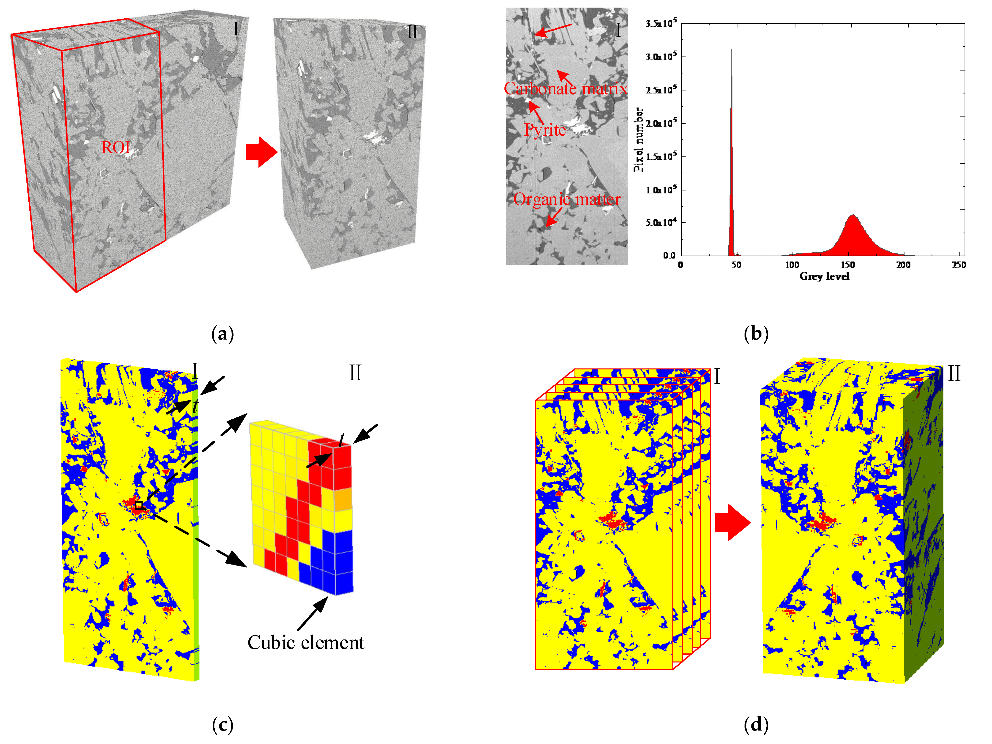
 organic matter,
  carbonate minerals,
  pyrites).
organic matter, carbonate minerals, pyrites).
pyrites).
organic matter, carbonate minerals, pyrites).
 organic matter,
  carbonate minerals,
  pyrites,
  damage elements,
  fractures).
organic matter, carbonate minerals, pyrites, damage elements, fractures).
fractures).
organic matter, carbonate minerals, pyrites, damage elements, fractures).
 organic matter,
  clay minerals,
  carbonate minerals).
organic matter, clay minerals, carbonate minerals).
carbonate minerals).
organic matter, clay minerals, carbonate minerals).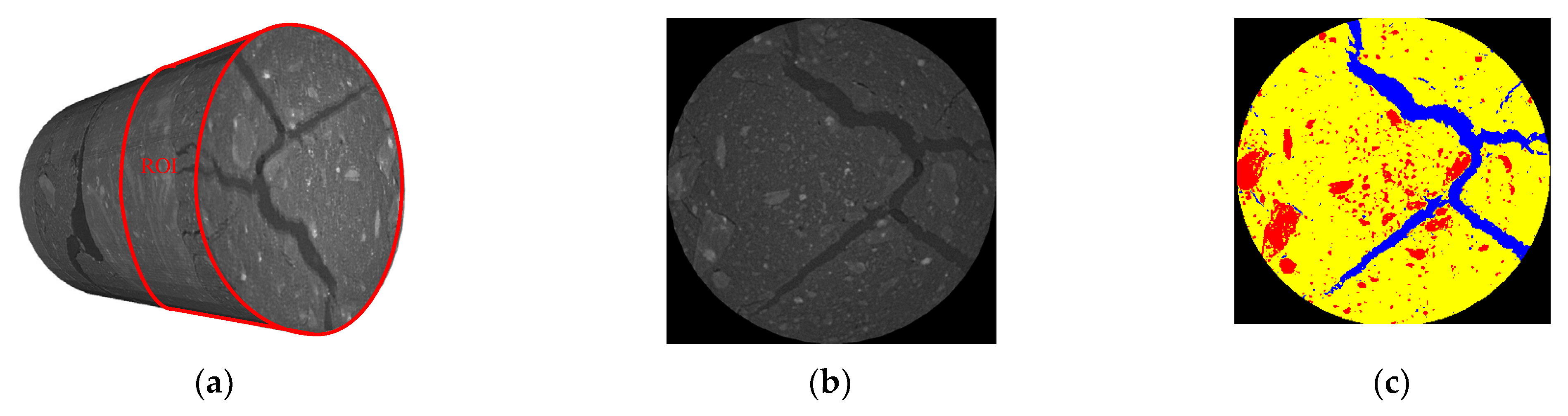
 organic matter,
  clay minerals,
  carbonate minerals).
organic matter, clay minerals, carbonate minerals).
carbonate minerals).
organic matter, clay minerals, carbonate minerals).
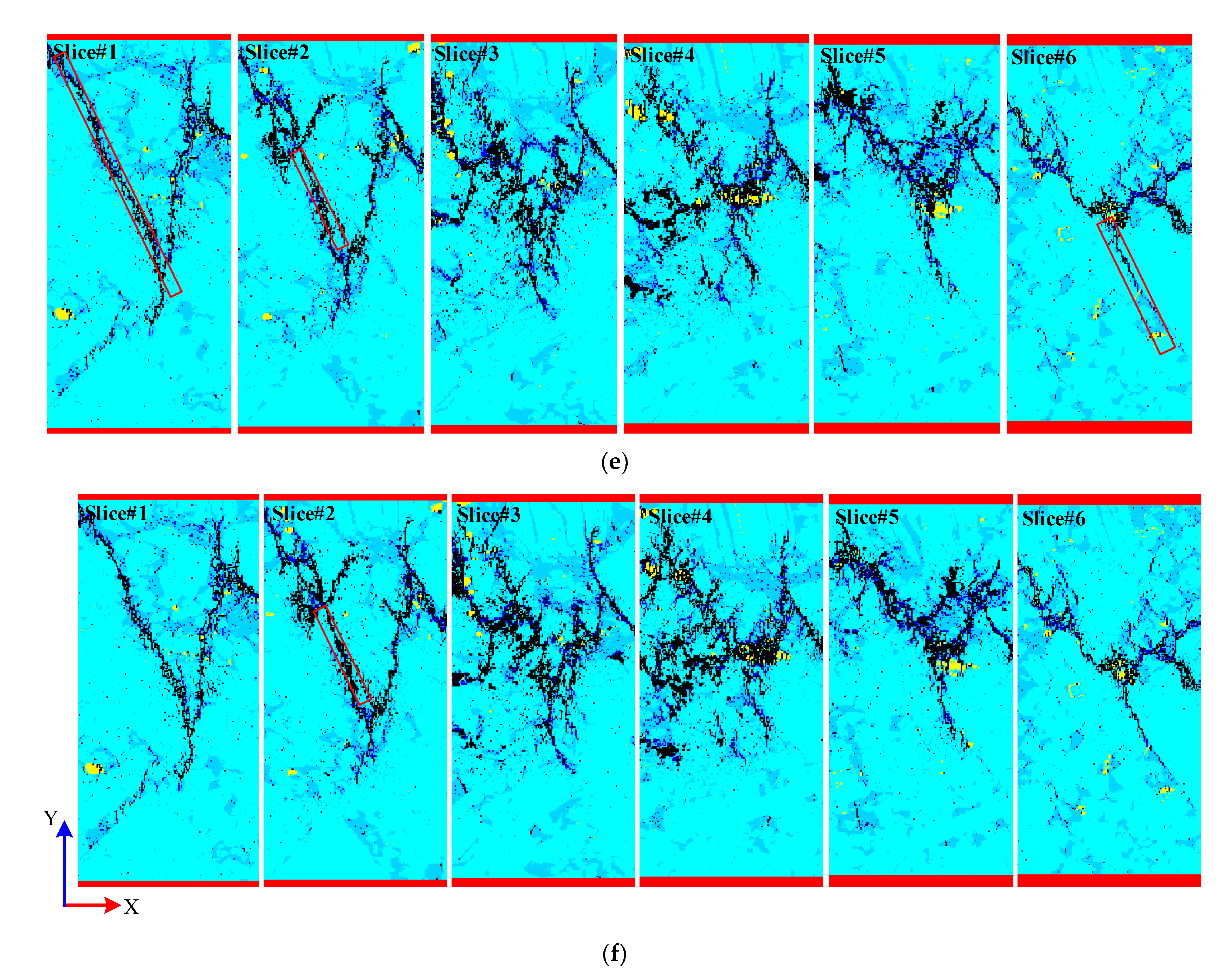
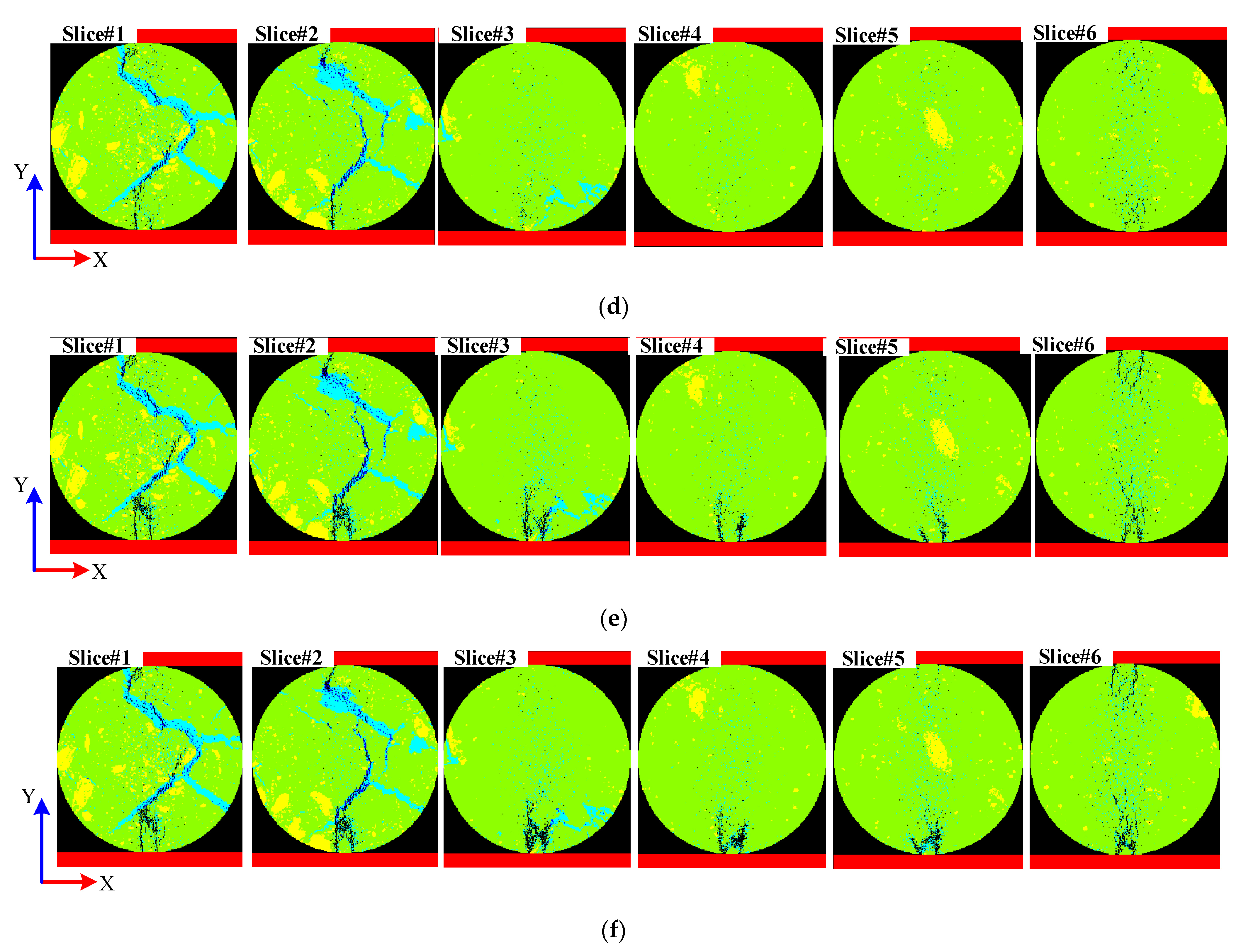
 organic matter,
  clay minerals,
  carbonate minerals,
  damage elements, fractures).
organic matter, clay minerals, carbonate minerals, damage elements, fractures).
damage elements, fractures).
organic matter, clay minerals, carbonate minerals, damage elements, fractures).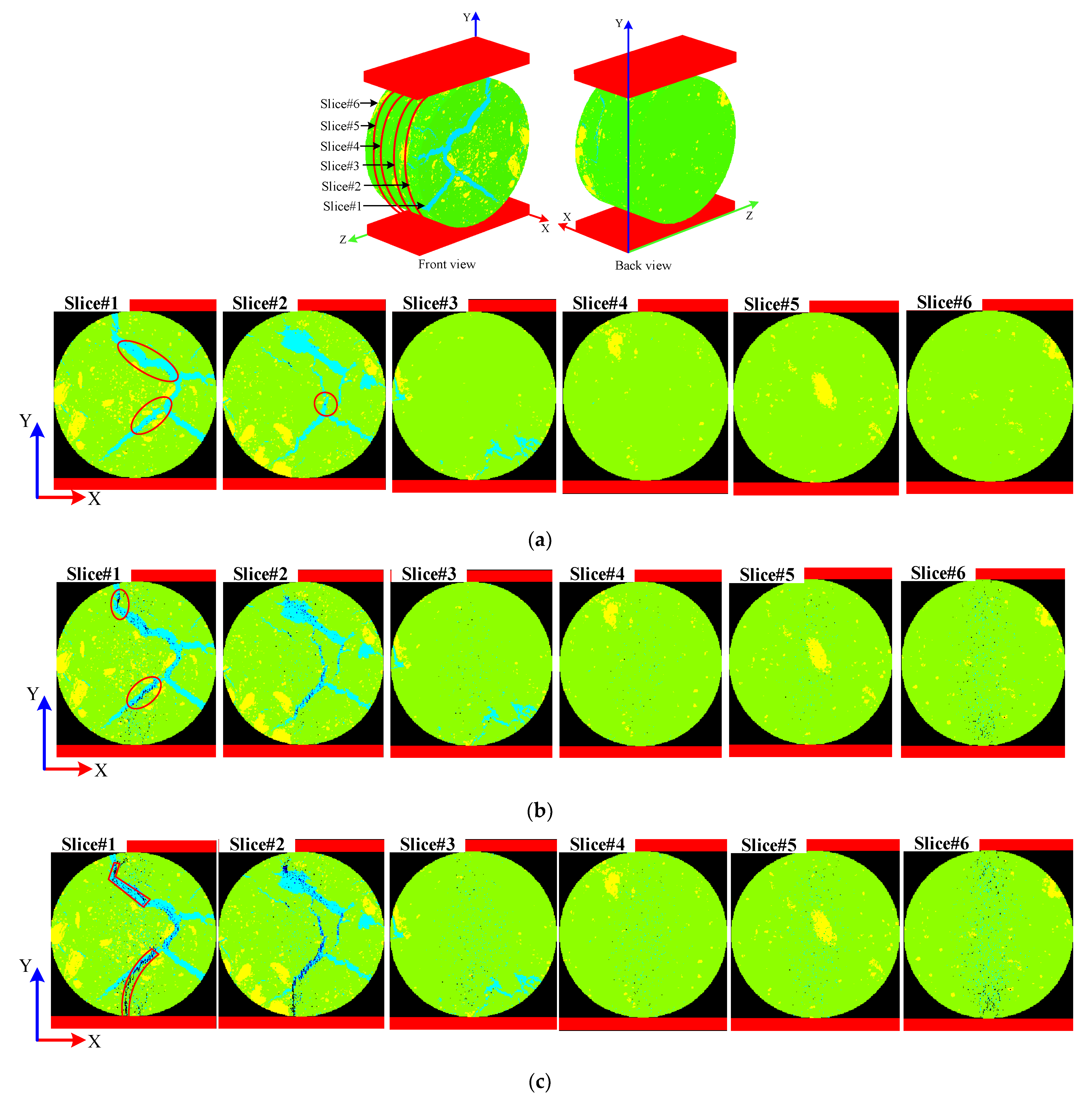


| Materials | [43,44,45]. | m | (°) | C/T | ||
|---|---|---|---|---|---|---|
| Organic matter | 20,000 | 60 | 2.5 | 0.34 | 35 | 10 |
| Clay | 59,000 | 155 | 2.8 | 0.32 | 35 | 10 |
| Carbonates (calcite) | 70,000 | 190 | 3 | 0.31 | 35 | 15 |
| pyrite | 90,000 | 310 | 5 | 0.19 | 35 | 15 |
| Materials | m | (°) | C/T | |||
|---|---|---|---|---|---|---|
| Rock matrix | 65,100 | 280 | 2 | 0.21 | 38 | 10 |
| Joint | 1160 | 10 | 3 | 0.31 | 30 | 12 |
Publisher’s Note: MDPI stays neutral with regard to jurisdictional claims in published maps and institutional affiliations. |
© 2022 by the authors. Licensee MDPI, Basel, Switzerland. This article is an open access article distributed under the terms and conditions of the Creative Commons Attribution (CC BY) license (https://creativecommons.org/licenses/by/4.0/).
Share and Cite
Liu, X.; Liang, Z.; Meng, S.; Tang, C.; Tao, J. Numerical Simulation Study of Brittle Rock Materials from Micro to Macro Scales Using Digital Image Processing and Parallel Computing. Appl. Sci. 2022, 12, 3864. https://doi.org/10.3390/app12083864
Liu X, Liang Z, Meng S, Tang C, Tao J. Numerical Simulation Study of Brittle Rock Materials from Micro to Macro Scales Using Digital Image Processing and Parallel Computing. Applied Sciences. 2022; 12(8):3864. https://doi.org/10.3390/app12083864
Chicago/Turabian StyleLiu, Xin, Zhengzhao Liang, Siwei Meng, Chunan Tang, and Jiaping Tao. 2022. "Numerical Simulation Study of Brittle Rock Materials from Micro to Macro Scales Using Digital Image Processing and Parallel Computing" Applied Sciences 12, no. 8: 3864. https://doi.org/10.3390/app12083864
APA StyleLiu, X., Liang, Z., Meng, S., Tang, C., & Tao, J. (2022). Numerical Simulation Study of Brittle Rock Materials from Micro to Macro Scales Using Digital Image Processing and Parallel Computing. Applied Sciences, 12(8), 3864. https://doi.org/10.3390/app12083864