Expanding the Sediment Transport Tracking Possibilities in a River Basin through the Development of a Digital Platform—DNS/SWAT

Abstract

Simulation of stochastic and variable sediment transport processes within models still poses a big challenge, especially in mountainous areas. Since sediment transport, including erosion and deposition, remains an unceasing problem in many areas, sediment modeling is perceived as a possible solution. This article combines a review of the selected sediment models with a presentation of the effects of several years of research using the DNS digital platform in the Western Carpathians. The review focuses on the main advantages and gaps in selected modeling tools with particular emphasis on one of the most popular: SWAT. The description of the digital platform—DNS is an example of how to answer these gaps by combining subsequent models, methods, and databases using their best features. To accentuate the benefits of such an approach, the effects of combining subsequent models (AdH/PTM) and methods (fingerprinting) on a common digital DNS space are presented, on the example of the Raba River (basin). In this way, both unique possibilities of estimating the amount of contamination carried with sediment particles and their sources, as well as sequencing of sedimentation in the reservoir, taking into account its subsequent zones, were obtained.

1. Introduction

Sediment transport is one of the most important processes for the mass movement of soil particles within a basin area. The driving force behind this process is primarily surface runoff in the land phase and flows in the channel network in the riverbed phase [1,2]. In practice, this concept covers both transport and the erosion that initiates it [3], and the deposition that concludes it [4,5]. This process is of great importance due to its social, ecological, and economic effects [6]. It is also highly sensitive to changes in land use, climate, river regulation, operation of hydrotechnical devices, and dam reservoirs [4,5]. These are some of the main reasons why sediment transport is becoming more and more non-linear in both time and space. Their consequence is a decrease in the depth, fertility and productivity of soils, a decrease in the river’s capacity, a shortened life of dam reservoirs, and thus, an increase in the risk of flooding [7]. Not surprisingly, in recent decades, this process has become an important topic on the agenda of local, national, and European policy makers, and is of scientific interest [8,9,10,11,12]. Sediment particle tracking is now one of the priority problems for water management, and environmental models were quickly identified as a possible solution [5,13,14,15,16]. This task was seemingly simple, but it quickly became clear that river basins are dynamic and complex systems, and the processes responsible for the transport of sediments in each of the phases are stochastic and variable [17]. In mountainous areas, the problem becomes even more complicated. Observational periods are usually short [17,18,19], and the system of channels and rivers is often cut off by anti-erosion structures and dam reservoirs, which retain almost all, especially coarse-grained sediments transported by the riverbed, thus interrupting the sediment continuum and losing river connectivity [20].

Over the last 15 years, there has been a dynamic increase in the use of computer applications, as evidenced by the number of articles on qualitative modeling published in scientific journals during this period, which has exceeded more than 3000 [21]. A rapid development of mathematical tools occurred and with it, this field of knowledge also created new possibilities for research on the transport of sediments. Currently, a wide range of sediment models are available, which differ in complexity, accuracy, inputs and outputs, approaches, and their spatial and temporal scales, which can be broadly classified as empirical (e.g., USLE, RUSLE, TMDL), conceptual (e.g., HSPF, AGNPS, SWAT), physical (e.g., KINEROS, MIKE-SHE, WESP), and hybrid (e.g., IHACRES-WQ, SEDNET) [3,22]. The achievements of these models in simulating sediment yield and sediment load are at least satisfactory (e.g., [23,24,25,26,27,28]). Nevertheless, the possibilities of considering the high affinity of fine-grained sediment fractions (<63 μm) with pollutants (e.g., heavy metals and nutrients) are still limited [29]. As a consequence, even the most advanced models often make it impossible to identify the sources of sediment within the basin [30], and to predict the risk of increased levels of pollution in rivers and water bodies [31,32,33,34,35]. Difficulties also exist in basins with a dam reservoir, which together constitute an integral dynamic system with deep interactions. These two elements of the basin area are usually studied using tools operating at different spatial and temporal scales, often treating them as separate units, or largely generalizing the relationships between them. The best solution to these problems seems to be the integration of both individual models as well as methods and databases. The primary goal of such integration is to combine fragmented knowledge to strengthen the ability to rigorously assess hypotheses and system responses in dynamic scenarios [36]. Model integration is usually difficult and limited by specific model code as well as formats and data exchange between models. Despite these difficulties, attempts have been made to make such connections. They often relate to extending the potential of models such as SWAT (Soil and Water Assessment Tool) [37,38,39], which is one of the highest rated tools in terms of water-quality modeling on the basin scale [21]. Until now, SWAT has been combined with models such as UCA2D-SCILA [40], EFDC [41], SOBEK [42], CLUE-S model [43] or HSPF [44], and methods such as remote sensing and image analysis—OBIA [45] or fingerprinting [30,46]. The combination and use of the best features of the available tools, grouped in one digital space, therefore seems to be an opportunity especially for mountainous areas, which are more difficult to model and particularly vulnerable to soil loss, such as the Western Carpathians. This area is one of the important soil erosion “hot spots” in Europe [47,48,49,50], and covers the area of Slovakia and Poland, as well as parts of the Czech Republic, Hungary, and Austria. The Western Carpathians were characterized by dynamic changes which today have a significant impact on both the land and the riverbed phases of this area. A strong drive to use the riverside land in agriculture and to protect the valleys against floods meant that from the second half of the 20th century, extensive regulatory work was carried out in the Polish part of the Western Carpathians, which consequently led the river to become much narrower, simpler, and shorter [51]. The result of this man-made process was a significant increase in riverbed erosion [52,53,54]. Moreover, the transformation of the centrally planned economy into a free market economy, which took place in 1989, resulted in a decrease in the profitability of agricultural production and its successive replacement with forested areas, thus limiting water erosion and surface runoff in the land phase [48,55]. For several years, attempts have been made to track the sediment transport in this area in both phases of the river basins. Erosion and sediment yield analyses focused on the use of both the digital elevation model (DEM) [56], commonly known empirical models (e.g., Universal Soil Loss Equation—USLE and its modifications MUSLE and RUSLE) [52,57], and more advanced environmental models, such as SWAT [58,59]. It is much more difficult to find examples of the use of models to simulate sediment transport in the riverbed phase. Earlier analyses of sediment transport in this area for this phase were mainly based on the results of in situ research [19,60,61,62].

The aim of this article is to present the current state of knowledge in the field of interdisciplinary studies of sediment transport in the basin area, with a particular emphasis on the mountain areas of the Western Carpathians. The manuscript presents the possibilities of using the developed digital platform—DNS (Discharge-Nutrient-Sea) with a SWAT module, to track soil particles from the source to the deposition in the pilot basin of the Raba River located in the Polish part of the Western Carpathians. This basin, due to its dual character and presence of a dammed reservoir, highlighted both the strengths and weaknesses of SWAT. This allowed to evaluate the possibilities and effectiveness of combining models, methods, and databases as further modules of the digital platform, expanding the possibilities and reducing limitations in tracing sediments both in the land and riverbed phase.

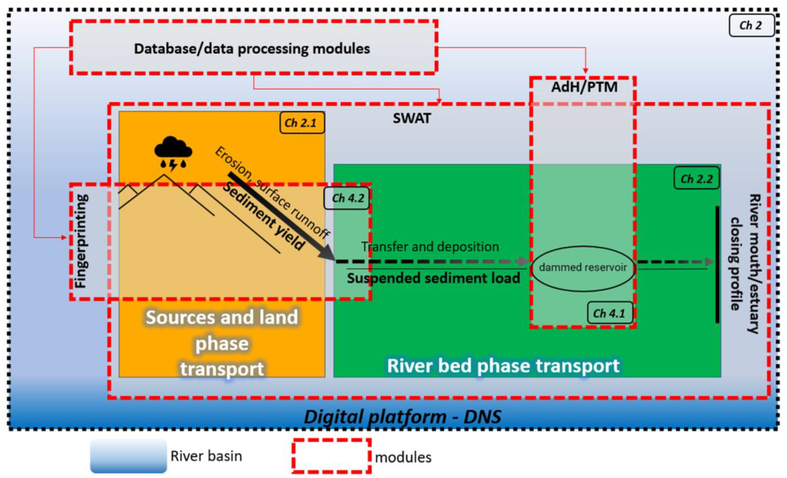
2. Digital Platform—DNS with SWAT Module

The digital platform—DNS was developed at the Polish Institute of Meteorology and Water Management—National Research Institute (IMGW-PIB). The decisive factor in its development was the ability to use the best features of models, methods, and databases concentrated in one digital space (Figure 1). Initially, the digital platform—DNS was used to simulate the transport of nutrients in basins with limited hydrological and qualitative monitoring data. This was made possible by combining the SWAT model and e.g., MIKE 11 [63], as well as IMWM-PIB monitoring databases and data-processing modules for supplementing missing measurement data, which was described in detail in [64,65,66,67]. SWAT has quickly become the most important module of the digital platform—DNS. It is a physical, semi-distributed continuous-time model that runs on a daily, monthly, or yearly time step. Its basic feature is the possibility of continuous simulation of hydrological processes (evapotranspiration, surface runoff, percolation, return flow, groundwater flow, transmission losses in the canal, retention in ponds and reservoirs, channel routing, and field drainage). However, SWAT can also simulate the transport of soil particles, both in the land and riverbed phases [68,69]. This feature quickly proved to be useful when trying to track sediment particles in the mountain basin in the Polish part of the Western Carpathians [70,71,72,73]. The key to a reliable simulation of sediment transport in SWAT is the appropriate quantity and quality of parameters and input data. Their task is to best represent the basin area with its natural and anthropogenic processes in the digital model space. The advantage and disadvantage of this tool is that it requires both the knowledge of a large number of parameters and the collection of appropriate input data [38,74].

SWAT was developed in the USA and many of its default parameters must first be adapted to the local conditions of the analyzed basin and be kept within a realistic range of uncertainty. In turn, the input data should describe the basin’s topography, soil characteristics and distribution, land cover, and meteorological conditions in the basin area at an appropriate level of detail. The basic input data required to build this tool are:

• − A digital elevation model (DEM) for information on the watercourse stream network and length, drainage pattern of the watershed, channel width within the watershed, slope, and reach length;
• − A map of hydrographical divisions in order to divide the basin area into sub-basins;
• − land use maps and agrotechnical data for determining land cover classes;
• − A soil map—detailed data on soil types to identify soil classes and their physical properties such as available water content, soil texture, soil bulk density, hydraulic conductivity, and organic matter;
• − Meteorological data for precipitation, temperature, humidity, wind speed and direction, and solar radiation.

2.1. Land Phase

This phase is the main source of sediment in a majority of basins, which is directly related to rainfall and runoff energy [75,76], which have a decisive influence on the phenomena of detachment and initiation of soil particle transport. The two most important processes that occur in this phase are surface runoff and erosion (detailed in Chapters 2.1.1 and 2.1.2), with soil type and land use being the most important responders. The SWAT module takes these responses into account by dividing the basin into areas with unique land use, soil, and slopes, creating so-called hydrological response units (HRU). For each HRU, the individual hydrological components of the land phase, such as rainfall, surface runoff, and evapotranspiration, are then simulated. The basis here is the water balance Equation (1), which was described in detail in the theoretical SWAT documentation [77]. Based on the daily components of the hydrological cycle the daily water budget in each HRU is calculated [37,78,79,80,81].

$$S{W}_t=S{W}_0+{\displaystyle \sum }_{i=1}^t\left(R_{day}-Q_{surf}-E_a-w_{seep}-Q_{gw}\right)$$

(1)

where: SW_t is the final soil water content, SW₀ is the initial soil water content, R_day is the amount of precipitation, Q_surf is amount of surface runoff, E_a is the amount of evapotranspiration, W_seep is the amount of water entering the vadose zone from the soil profile, and Q_gw is the amount of return flow (all in mm H₂O).

The SWAT module has been successfully used many times around the world to simulate sediment yield transport in the land phase of the basin area, as confirmed by numerous publications (e.g., [82,83,84]). Nevertheless, there are some limitations to both the data and the module itself. These include the common problem with the unavailability of data on sediment yield efficiency [85]. In practice, this causes situations where the time step of sediment calibration and validation is different than for hydrology, for which monitoring data are usually more readily available even for smaller basins. This reduces the accuracy of the model in the simulation of the land-phase sediment yield. The problem is also the generalization of the SWAT model, the effect of which is, for example, allowing all eroded soil to reach the riverbed with surface runoff (without taking into account sedimentation still in the land phase), as well as simulation of sediment-bound pollutants, determined by the primary concentration of nutrients in the soil, soil loss, and the soil coefficient enrichment, which is often not applicable in many basins [86]. Another limitation of the model in this phase is the use of numerous empirical and quasi-physical equations developed on the basis of climatic conditions in the USA [87], including simplified sediment routing algorithms for erosion simulation [84,88,89].

2.1.1. Surface Runoff

Accurate determination of surface runoff is critical in estimating sediment transport in the land phase of the basin [90,91]. The SWAT module helps to estimate surface runoff, taking into account the related transport of organic and inorganic pollutants [92]. In this tool, it is possible to choose one of two methods of estimating this phenomenon: the Green and Ampt infiltration method [93,94], and the Soil Conservation Service Curve Number (SCS-CN) procedure [95]. The physical method of Green and Ampt assumes a sharp wetting front during infiltration with saturated soil above the unsaturated zone [96]. Nevertheless, the popularity of this method is much lower due to the required high time resolution of the input data on precipitation (time step less than 24 h) [97,98]. The SCS-CN empirical model (2 and 3), which is mainly based on soil properties, land use, and hydrological conditions, is widely used for surface runoff estimation with daily precipitation as input.

$$Q_{surf}=\frac{{\left(R_{day}-0.2S\right)}^2}{\left(R_{day}+0.8S\right)}$$

(2)

where: Q_surf is the daily surface runoff (mm), Rday is the rainfall depth for the day (mm), and S is the retention parameter (mm). The retention parameter S and the prediction of lateral flow by SWAT model are defined in Equation (3):

$$S=25.4 \left(\frac{1000}{CN}-10\right)$$

(3)

where: S is the drainable volume of soil water per unit area of saturated thickness (mm/day), and CN is the curve number.

However, confidence in SCS-CN results should be limited [99,100] because this method causes problems with underestimating peak flows in relation to monitoring data (e.g., [84,101]). One of the causes is that the constant initial abstraction is used as an intrinsic parameter, which may result in inconsistency of the soil moisture accounting. In addition, the duration and intensity of rainfall are not considered; instead, the average daily rainfall is used as a SWAT input. In fact, high-intensity and even short-duration rainfall could generate more sediment than actualized in the model based on daily rainfall [86]. Therefore, after selecting this method, it is important to perform, in addition to the statistical evaluation of the model, a visual evaluation of the results, allowing a more intuitive way to characterize the model’s ability to recreate the characteristics of the flow regime for a given basin area, especially floods and low flows. The few available studies [97] generally suggest that the Green and Ampt method works better for stream flow and avoids the limitations of the SCS method. The requirements for high-resolution precipitation data can be met by precipitation atlases containing accurate data from many years with a step for even every 10 min, which has already been prepared and described for the all territory of Poland by [102,103].

2.1.2. Erosion

Erosion is a key process that initiates the transport of sediment particles down the basin. At the same time, it is one of the most serious problems of environmental degradation, adversely affecting many natural and man-made ecosystems [104]. In agricultural basins, soil erosion not only reduces the nutrient-rich topsoil in place, but also degrades water quality by moving sediment off site. An example of a compromise between empirical and physical algorithms in the SWAT module is the use of a modified Universal Soil Loss Equation (MUSLE) to predict soil erosion at the HRU level resulting in soil particle transport. MUSLE (4) is a modified version of USLE [105] based on the runoff characteristics as the best single indicator for predicting sediment performance at the basin outlet, and factors influencing soil erosion. By using the energy of surface runoff, not rainfall, MUSLE is suitable for use on a daily basis to estimate the sediment efficiency, and takes into account sediment deposition in HRU [106]. MUSLE eliminates the need for delivery ratios and allows the equation to be applied to individual storm events, and therefore improves prediction of sediment loading [84,107,108,109].

$$SY=11.8 {\left(Q_{qp}A\right)}^{0.56} \left(C P K LS F_{CRFG}\right)$$

(4)

where: SY = HRU sediment yield (t/day); Q = daily runoff volume (mm); qp = runoff peak discharge (m³/s); A = HRU area (ha); C, P, K, and LS are dimensionless factors accounting for HRU crop cover, soil protection, soil erodibility, and topography as defined in the original Universal Soil Loss Equation (USLE); and F_CRFG is a dimensionless factor to account for coarse fragment cover (stoniness).

Although the effectiveness of MUSLE in sediment transport analysis has been confirmed [109,110], it should be remembered that the quality and reliability of sediment simulations are not only directly related to runoff simulations, but also show high sensitivity to rainfall characteristics. The kinetic energy of the raindrops plays an important role in soil detachment, but also causes runoff disturbance. Ignoring them by the SWAT module, in the case of some basins, may lead to a deterioration in the adjustment of simulated data to real conditions [111].

2.2. Riverbed Phase

This phase controls the movement of water and suspended sediment generation through the channel network of the watershed to the outlet [81,112,113]. The water is routed through the main canal network using the Muskingum routing method using Manning’s Equation (5), and the suspended sediment transported with the water is subject to deposition and degradation processes (6–9) [114]. These two processes are computed with a simplified version of the Bagnold stream power equation, where the maximum amount of sediment transported from each sub-basin is a function of the peak channel velocity. If the concentration of sediment in the basin area, at the beginning of the time step, exceeds the maximum concentration of sediment that can be transferred by the water, additional sediment is deposited; if not, degradation occurs, which is a function of the channel erosion and the channel vegetation cover [115].

The average flow velocity, v_ch (m/s), is calculated using Manning’s equation:

$$v_{ch }=\frac{R_{ch}^{2/3}*sl{p}_{ch}^{1/2}}{n}$$

(5)

where: $sl{p}_{ch}^{}$ is the riverbed phase of each sub-basin slope (m/m), and $n$ is the Manning coefficient.

The maximum concentration of sediment that can be transported through in the riverbed phase of each sub-basin is closely related to the peak channel velocity at the daily time step. The peak channel velocity (m/s) and the maximum sediment concentration are calculated as:

$$v_{ch,pk}=PRF* v_{ch}$$

(6)

$$con{c}_{sed,ch,mx}=C_{sp}* v_{ch,pk}^{spexp}$$

(7)

where: $PRF$ is the peak rate adjustment factor, $v_{ch}$ is the mean flow velocity, $C_{sp}$ is a coefficient, and $spexp$ is an exponent.

The $con{c}_{sed,ch,mx}$ (t/m³) is compared to the actual concentration of sediment in the riverbed phase of each sub-basin (t/m³). If $con{c}_{sed,ch,i}$ > $con{c}_{sed,ch,mx}$, deposition dominates in the riverbed phase of each sub-basin, sediment routing and the sediment deposition $se{d}_{dep}$ is calculated as:

$$se{d}_{dep}=\left(con{c}_{sed,ch,i}-con{c}_{sed,ch,mx}\right)*Q_{ch}$$

(8)

However, if $con{c}_{sed,ch,mx}$ > $con{c}_{sed,ch,i}$, degradation or erosion dominates in the riverbed phase of each sub-basin, sediment routing and the sediment degradation $se{d}_{deg}$ is calculated as:

$$se{d}_{deg}=\left(con{c}_{sed,ch,i}-con{c}_{sed,ch, mz}\right)*Q_{ch}*K_{ch}*C_{ch}$$

(9)

where: $K_{ch}$ is the erodibility factor in the riverbed phase of each sub-basin, and $C_{ch}$ is the cover factor in the riverbed phase of each sub-basin.

However, the Bagnold equation, the default in the SWAT module, is considered impractical to apply across the entire streaming network [116]. The SWAT module also offers three alternative sediment tracking methods to the Bagnold method (Kodoatie, Molinas and Wu, and Yang Sand and Gravel). All these equations share the same in-stream sediment routing (sediment transport capacity is routed in main reaches/channels), but calculate the maximum sediment transport capacity (maximum concentration of transportable sediment) differently [117], and allow for the analysis of individual sediment fractions. The Yang equation was developed to simulate large particles such as sand and gravel. The Molinas and Wu equation and the Kodoatie equation are better suited for simulating small particles forming suspended sediments. In all four equations, bed erosion exceeded bank erosion [118,119,120]. Despite this choice of equations for sediment tracking in the riverbed phase, studies show that SWAT does not have a solid representation of the sediment processes in the stream [121]. The mechanisms associated with the transport of cohesive and non-cohesive sediment fractions in stream systems are different. The mentioned empirical and physical methods implemented in SWAT for the erosion, deposition, and transport of sediment in a stream system are universally applied across all sediment fractions. Consequently, a careful and critical approach to the obtained results must be exercised, especially in the case of the basin area in which the riverbed has been identified as the main source of sediment [44,122].

3. Using the Digital Platform—DNS/SWAT

In order to track suspended sediment transport in the land and riverbed phase of the pilot basin, the most important SWAT module was used on the digital platform—DNS, which was supported by data processing (LOAD ESTimator), and database modules (meteorological and land use). The use of the United States Geological Survey (USGS) FORTRAN—LOAD ESTimator program [123] made it possible to take into account the sediment concentration in, i.e., extreme flow situations, using the available interpolated sediment observations to fill the time gaps. LOADEST provides an estimate of the sediment load as a function of the observed daily river flow. This function is determined by performing a linear regression analysis between the available sediment concentration observations and the corresponding river flow data. In turn, the database module (meteorological and land use) made it possible to take into account the data on the current and future average monthly temperatures, and precipitation [124], as well as the results of the FORECOM project for the entire area of the Polish part of the Western Carpathians [125], taking into account the forecast changes in land use. This allowed for the creation of variant scenarios and the study of the effects of changing one, or several parameters over time.

The Raba basin area, which is over 131 km long, is part of the Polish Western Carpathians. Its sources are located in the Gorce mountain range at an altitude of 780 m a.s.l., and the estuary to the Vistula River at a height of 180 m a.s.l. [126,127]. The choice of this basin for research with the use of the digital platform—DNS/SWAT was related, i.e., by its dual nature and location (Figure 2). The mountainous nature of its upper part manifests itself in a quick reaction to rainfall and high dynamics of surface runoff. On the other hand, in the lower part, as the height of the slopes decrease, the amount of precipitation and the dynamics of surface runoff also decrease [128]. It is also an area dominated by agriculture, which further contributes to soil loss in the area. The Raba riverbed phase is complex. The main bed runs through the bottom of an alluvial valley and is characterized by a relatively steep slope, a significant inflow of sediments from the slopes, and frequent floods [128,129,130]. Moreover, features of the basin area, such as its location in an area particularly exposed to water erosion, the proximity to one of the largest Polish urban agglomerations—Krakow, and the presence of a dam reservoir halfway along the river, make both quantitative and qualitative tracking of sediments a challenge.

The land use (CLC, 20 m resolution), soil types (1:5000, IUNG, 2.5 m resolution), and slopes, made it possible to divide the analyzed area into a total of 902 HRU. for which the calculations were performed. Then they were aggregated to a level of 36 sub-basins (Figure 2) with an average area of 4214 ha, determined on the basis of DEM (1:20,000, IMWM-PIB), and maps of hydrographic divisions (1:10,000, IMWM-PIB). Meteorological conditions were represented in the model, on the basis of data, on precipitation, temperature, solar radiation, humidity, and wind directions from 1992–2016 from 75 meteorological stations (IMGW-PIB). Access to the data of the Dobczyce dam reservoir (area, volume, maximum and minimum daily runoff, water damming height, as well as concentration and diameter of sediment particles in the reservoir) came from field studies.

The model calibration (Myślenice and Proszówki) and validation process (Stradomka) and the preceding sensitivity analysis were carried out using the SWAT-CUP program [131], and the SUFI-2 algorithm [39,132]. The SUFI-2 algorithm tries to capture as many optimal simulations as possible that are within the 95% prediction certainty. The algorithm does not obtain a unique value for the parameters, but an interval that includes all the uncertainties of the processes in the basin. The sensitivity analysis allows us to assess the reaction of the model to the change of input parameters, allowing us to identify the most important parameters of the model for the analyzed basin. The sensitivity of parameters is measured using t-stat values, where the values are more sensitive to larger absolute values. The p-values are used to determine the significance of the sensitivity when the parameter becomes significant if the p-values are close to zero [132].

Most of the parameters selected by the sensitivity analysis are the same for both the upper and lower parts of the Raba basin, but their significance for sediment transport simulation differs (

Table 1. Calibration of SWAT parameters for the upper and lower Raba basin sorted by t-stat.

Parameter Name	Definition	t-Stat	p-Value
mountain area—Upper Raba
SURLAG.hru	Surface runoff lag coefficient	−1.04	2.98 × 10−1
USLE_K(1).sol	USLE equation soil erodibility (K) factor	−7.02 × 10−1	4.83 × 10−1
SOL_K(1).sol	Saturated hydraulic conductivity	−4.45 × 10−1	6.56 × 10−1
PRF_BSN.bsn	Peak rate adjustment factor for sediment routing in the main channel	−3.98 × 10−1	6.91 × 10−1
CH_K2.rte	Effective hydraulic conductivity in the main channel alluvium	−3.10 × 10−1	7.57 × 10−1
ESCO.hru	Soil evaporation compensation factor	−2.45 × 10−1	8.07 × 10−1
SPEXP.bsn	Exponent parameter for calculating sediment reentrained in channel sediment routing	4.23 × 10−2	9.66 × 10−1
CH_COV1.rte	Channel erodibility factor	1.07 × 10−1	9.14 × 10−1
CH_COV2.rte	Channel cover factor	1.46 × 10−1	8.84 × 10−1
ADJ_PKR.bsn	Peak rate adjustment factor for sediment routing in the subbasin	8.07 × 10−1	4.20 × 10−1
SPCON.bsn	Linear parameter for calculating the maximum amount of sediment that can be reentrained during channel sediment routing.	8.93 × 10−1	3.72 × 10−1
SOL_AWC(1).sol	Available water capacity of the soil layer	1.37	1.72 × 10−1
CH_N2.rte	Manning’s “n” value for the main channel	5.51	5.79 × 10−8
USLE_P.mgt	USLE equation support practice	7.49	3.41 × 10−13
CN2.mgt	Initial SCS runoff curve number for moisture condition	1.62 × 101	4.30 × 10−47
HRU_SLP.hru	Average slope steepness	2.08 × 101	8.70 × 10−69
submountain area—Lower Raba
GW_DELAY.gw	Groundwater delay time	−1.47	1.43 × 10−1
USLE_P.mgt	USLE equation support practice	−1.17	2.43 × 10−1
SURLAG.hru	Surface runoff lag coefficient	−1.02	3.10 × 10−1
USLE_K(1).sol	USLE equation soil erodibility (K) factor	−3.20 × 10−1	7.49 × 10−1
SPEXP.bsn	Exponent parameter for calculating sediment reentrained in channel sediment routing	4.23 × 10−2	9.66 × 10−1
CH_COV2.rte	Channel cover factor	7.53 × 10−2	9.40 × 10−1
RES_SED.res	Initial sediment concentration in the reservoir	6.18 × 10−1	5.37 × 10−1
CN2.mgt	Initial SCS runoff curve number for moisture condition	8.70 × 10−1	3.85 × 10−1
SPCON.bsn	Linear parameter for calculating the maximum amount of sediment that can be reentrained during channel sediment routing	8.93 × 10−1	3.72 × 10−1
ADJ_PKR.bsn	Peak rate adjustment factor for sediment routing in the subbasin	1.08	2.81 × 10−1
CH_COV1.rte	Channel erodibility factor	1.17	2.41 × 10−1
RES_RR.res	average daily principal spillway release	1.17	2.41 × 10−1
PRF_BSN.bsn	Peak rate adjustment factor for sediment routing in the main channel	1.46	1.45 × 10−1
ALPHA_BF.gw	Baseflow alpha factor	1.62	1.07 × 10−1
RES_NSED.res	Normal sediment concentration in the reservoir	2.42	1.59 × 10−2
HRU_SLP.hru	Average slope steepness	5.84	9.90 × 10−9

). In mountainous areas, surface runoff (SURLAG), followed by soil erosion (USLE_K) and the value of saturated conductivity (SOL_K), which is a parameter controlling surface runoff, have the greatest impact on sediment transport simulations. In addition, specific only to the upper Raba are parameters such as the soil evaporation compensation factor (ESCO), and available soil water capacity (SOL_AWC) responsible for the so-called surface response. In contrast, in the sub-mountainous area, groundwater processes (GW_DELAY), and the ratio of soil loss within a specific support practice (e.g., contour tillage, strip tillage) to the corresponding up-and-down cultivation loss (USLE_P) have the greatest impact. The surface runoff (SURLAG) came in third. Characteristic only for this part of the basin area are the parameters responsible for the so-called subsurface response (GW_DELAY, ALPHA_BF), and reservoir parameters (RES_SED, RES_RR, and RES_NSED), which shows the important influence of a dam reservoir on the hydrology of the basin and, consequently, on sediment transport.

Model calibration for the flow and sediment was carried out in the calculation profiles of Myślenice (upper part) and Proszówki (lower part), and validation for the Stradomka river, which is the right-bank tributary of the Raba. The low frequency of sediment concentration monitoring (12 times a year) was the reason why LOAD ESTimator was used to develop a regression model to reliably estimate loads. Four statistical measures were used to assess the correctness of this process: coefficient of determination (R²) [133], the efficiency of the Nash–Sutcliffe (NSE) [134], the percentage of bias (PBIAS) [15], and Kling’s efficiency-Gupta (KGE) [134]. Using the ranges of values for these statistical measures (Table S1), the degree of matching of the simulation results to the observed data was assessed (Table S2). On this basis, the model was considered calibrated and validated at a level that allows the use of this tool to track sediment particles in the basin area. The entire procedure is described in detail in [135].

3.1. Sediment Yield—Land Phase Simulation

Transport of sediment in the land phase of the basin in the SWAT module consists of simulating the mass of the sediment leaving individual area units (HRU) using the MUSLE (2) equation per time and per unit area, known as sediment yield (SYLD) [135]. HRUs allow the spatial heterogeneity of land use, soil, and slope to be taken into account, increasing the accuracy of SYLD forecasting, which is of particular importance in distinctly dual character basins such as the Raba. The basin area is often considered the most important explanatory factor for SYLD, due to the reduction in the rate of topsoil erosion on smaller slopes and the increased likelihood of sediment deposition as the basin area increases. In addition, especially in mountainous areas, SYLD is influenced by factors such as topography, land cover, reservoir effects, and climatic conditions. However, their relative importance in explaining the spatial variation of SYLD is still not fully understood, as it is specific to each basin area [136]. Analyses of regional SYLD patterns mainly concern larger river systems [137,138], and this further limits information on smaller basins that are often more important for sediment transport. The Western Carpathians, including the Raba River basin, can be called “hot spots” where, as a result of erosion, the transport of significant amounts of SYLD is initiated. Nevertheless, sediment yield monitoring in this area is very limited and was carried out for a limited time, only for individual tributaries of the Dobczyce dam reservoir [139]. Only the use of mathematical models has significantly increased the knowledge of the transport of sediment particles in the land phase throughout the Carpathian region [56,57,58,140,141]. The digital platform—DNS/SWAT made it possible to estimate the aggregated values of SYLD, being a function of the runoff processes, for each of the 36 Raba sub-basins, taking into account their temporal variability. Thus, spring was identified as the period of maximum average sediment yield values reaching 0.92 t/ha and 0.57 t/ha, and winter with minimum values of 0.28 t/ha and 0.21 t/ha for the upper and lower parts of the basin, respectively [138,142]. These studies can therefore both confirm the role of modeling as a reliable means of obtaining detailed information on the rate and amount of soil loss in areas such as the Carpathian region, and help understand the effect of basin factors such as slopes, land use, and soil type on the spatial variability of SYLD.

3.2. Suspended Sediment Load—Riverbed Phase

The analysis of the quantity and time variability of sediment load in the riverbed phase was a continuation of the tracking of soil particle transport in the land phase [71]. The SWAT module enables simulation of the sediment mass per time unit (sediment load), equal to the product of the flow rate and the concentration of sediment particles contained within it, on the calculation profile of the sub-basins (Figure 2). Contrary to SYLD, the concentration of sediment and the flow rate are among the basic parameters monitored by the SEM and the IMGW-PIB. This allowed the use of SWAT to estimate the sediment load flowing from both the upper (Dobczyce calculation profile) and the lower part of the Raba basin (Proszówki calculation profile) (Figure 2). The alternative Kodoatie method was selected for the calculations, which meant mainly tracking the fractions contained in the suspended sediment (<63 μm). Selected modifications to the riverbed, such as anti-erosion structures [143] and related disturbances in sediment transport, were also taken into account.

Ultimately, the application of the SWAT module made it possible to estimate the average load of suspended sediment flowing into the dam reservoir from the upper Raba area at 553 t/m [71]. It is worth noting that on the calculation profile of Proszówki, closing the lower part of the Raba basin (Figure 2), the suspended sediment load was estimated at an average level of 897 t/m. This is despite the dam reservoir that traps most sediment particles flowing into it from the upper Raba. However, this difference is justified and results both from the type of soil in the lower Raba, susceptible to erosion, and the dominant role of agriculture in this area, which, despite the lower slopes, favors soil loss.

The visual analysis of the results showed the negative effects of the SCS-CN method, forced by the daily time step of rainfall data for the Raba. As a result, despite the at least satisfactory results of the calibration and validation of the model (in Table S2), there are visible underestimations of the simulated values of the monitoring results, especially in the periods of peak flows (Figure 3), which also affects the matching of sediment loads.

4. Digital Platform—DNS/SWAT—New Modules

The next stage of the research was an attempt to answer questions about the places of deposition of individual sediment fractions in selected zones of the dam reservoir, and the pollution transported with sediment particles and their sources. Obtaining answers to these questions, however, exceeded the capabilities of a single SWAT module. The open nature of the digital platform—DNS allowed to use its possibilities of combining models (AdH—Adaptive Hydraulic Model)/PTM—Particle Tracking Model), and methods (fingerprinting) as further modules supplementing the SWAT limitations. In the area of the Western Carpathians, the capabilities of these tools were rarely used or not used at all. Limitations also applied to monitoring data. Therefore, the database module was also expanded with the results of soil measurements–s in the basin area, and continuous measurements of the suspended sediment made by the BS-2 suspended sediment sampler permanently installed on the Wolnica River (Figure 2), which is a tributary of the dam reservoir [72].

4.1. AdH/PTM

The SWAT module made it possible to simulate suspended sediment load transport in the analyzed Raba River basin, maintaining the continuity of this process between the upper and lower part of the basin, by taking into account the dam reservoir. So, it was possible to estimate the suspended sediment load both before and after the reservoir. However, this tool could not show the sequencing of sedimentation in the tank itself, divided into zones where this process occurs with varying intensity depending on the period and size of sediment particles [41]. Therefore, for this purpose, the AdH/PTM model was used, which was previously built and verified by the method of comparative analysis with real data [144,145]. AdH is a two-dimensional hydrodynamic modeling tool that uses the finite element method to solve two-dimensional equations of momentum conservation for water in the Euler system. On this basis, the particles’ behavior over time (entrainment, advection, diffusion, settling, deposition, burying, etc.) was simulated using the PTM module. At each time step, PTM performs calculations to determine the local characteristics of the environment and the behavior of each representative particle tracked. Their combination with the SWAT module on the DNS platform allowed for precise tracking of particles of individual suspended sediment fractions from their source, through transport, and ultimately their sedimentation in each of the four zones of the dam reservoir with a monthly time step [146]. The input data for the AdH/PTP module were the SWAT simulation results for the monthly mean values of the suspended sediments obtained in the previous study (Section 3.2). The functionality of the Kodoatie method was used to determine the size of the load of individual suspended sediment fractions (mineral: CLAY—0–0.004 mm; SILT—0.004–0.062 mm, and mineral/organic: SMAG—0.03 mm) flowing to the Dobczyce dam reservoir (Myślenice calculation profile), amounting to 1.11 t/m, 96.7 t/m, and 455 t/m, respectively. These particle masses of the individual fractions were characterized by essentially different deposition sites in the reservoir. In the case of SMAG, the highest percentage of particles belonging to this fraction was deposited in the summer months (June, July, and August) in the backwater zone and the Myślenice basin (from 26 to 47%, and 52 to even 70%, respectively). In the case of the SILT fraction, most of these particles were deposited in the first two zones; however, seasonality had a large impact on this process (river—from 42 to 71%, and backwater—from 27 to 48%). In the case of CLAY, a similar seasonal pattern was observed, but most of these particles were deposited in the backwater zone and the Myślenice basin (23–47% and 30–40%, respectively). However, most important were the results concerning the particles of this fraction reaching the dam itself, and further to the lower part of the basin (even from 46 to 60%). This poses a direct threat to, e.g., drinking water, the intake of which is located in the last zone of the dam reservoir. The described results, together with their seasonal changes, can be analyzed in detail for each fraction in the developed graphical database [147].

4.2. Fingerprinting

The effectiveness of the SWAT module in simulating the transport of sediment particles, especially in the land phase of the basin, has been repeatedly confirmed. However, the problem was the absorption capacity of the finer sediment particles, which are responsible for the transport of pollutants such as heavy metals [148]. SWAT itself has limited ability to simulate such pollutants, as well as the ability to use them to determine the contribution of individual sediment sources. The fingerprinting method [72] has already been successfully combined with SWAT, but without using all the possibilities offered by these tools [30,149,150]. The effectiveness of such integration of tools can be appreciated, especially in areas under the pressure of large emitters of pollutants [151]. This is one of the reasons why the Wolnica basin (a fragment of the Raba basin) was selected for study (Figure 2), located only 23 km from one of the largest urbanized areas in Poland. The Krakow agglomeration covers an area of approximately 3231 km² and is inhabited by approximately 1400 million people [152]; its concentration of particulate matter is one of the highest in Europe [153]. In the land phase of the Wolnica basin area, soil sampling sites were designated, and a suspended sediment sampler BS-2 (Figure 4) was installed in the riverbed phase at the estuary [72].

The results of these measurements broadened existing knowledge about this area and became part of the data module, which then fed the fingerprinting module. It was based on inputs from four sources of suspended sediments: grassland, forest, arable land, and residential areas, occurring in the Wolnica river basin. The research led to the selection of Pb, Zn, Cd, Cu, Ni, and Hg as the optimal fingerprints to solve the mass balance equation for suspended sediment and soil samples [72]. The temporal pattern of sediment yields for specific land-use types followed the SYLD distribution for the entire basin, with maximum values of 1.52 t/ha in May for grassland. The land-use sediment yields mainly reflected differences between surface areas for the particular land-use types, displaying the highest values of 139 t/m and 156 t/m for arable and residential land, respectively, and the lowest (2.3 t/m) for forest. Overall, adding the fingerprinting module to the digital platform—DNS/SWAT made it possible to demonstrate the dependence of SYLD distribution on meteorological and topographic conditions. Only in the case of forest areas can low SYLD values be expected. The fingerprint module shows that forests significantly change the signals of pollution sent by the system. Their location is important as they buffer the terrain-dependent flow of pollutants directly into the river.

5. Conclusions

This review explores the available mathematical tools for tracking sediment transport in river basins, especially considering problems in mountainous areas such as the Western Carpathians. Particular attention was paid to the limitations of using single models such as SWAT, and the possibility of eliminating them through the still-rare practices of combining subsequent models, methods, and databases/data processing in order to use their best elements. This article allows one to follow the effects of several years of research using the digital platform—DNS and its most important module—SWAT. This tool was designed to simulate, in a digital space, a model of many natural and anthropogenic processes in river basins responsible for the erosion, transport, and deposition of sediment particles. However, its effectiveness may be different for the land and riverbed phase of the basin area, which may have negative consequences in the form of limited confidence in the obtained results. SWAT also has limitations in tracking sediment deposition in dam reservoirs as well as particle-bound contaminant transfer. The use of the digital platform—DNS allowed us to broaden the spectrum of model research, first by combining the SWAT module with the fingerprinting method, and a database with a suspended sediment sampler. The result was a useful tool for tracking spatial and temporal changes in sediment yield and contaminants transported on soil particles. Both meteorological and topographic conditions were indicated as the main factors influencing the sediment yield distribution, as well as forest areas, which were the only ones distinguished by low SYLD values. In the next stage, the combined SWAT and AdH/PTM modules showed the temporal and spatial sequence of sedimentation in each zone of the dam reservoir, confirming its favorable layout and location that effectively protects the drinking water intake. The threats related to the growing amount of CLAY fraction, susceptible to pollutant absorption, reaching the last zone of the tank were also revealed. The open nature of the digital platform—DNS, and thus the possibility of using the available tools as subsequent modules provide the basis for the elimination of further limitations related to the tracking of sediment transport. Research results already available indicate that the highly uncertain simulation of sediments in the riverbed phase in the SWAT module could be successfully replaced by using a more robust physics-based approach from models such as HSPF [44]. Another problem is urbanized areas, the rapid development of which is difficult to represent in models due to the limited access of data constituting the basis for constructing variant scenarios. Meanwhile, a combination of tools such as SWAT and, for example, CLUE-S (Land Use Conversion and its Impact on a Small Regional Coverage) [43] may reduce these limitations. This will allow the effects of future land-use change scenarios to be simulated based on, inter alia, historical trends. Finally, there is a problem with database modules, especially those related to precipitation, whose current temporal resolution is insufficient and requires the use of less precise calculation methods. The solution may be the so-called precipitation atlases with high-resolution data added to the digital platform—DNS, which will significantly improve the quality of simulations in both phases of the basin. Despite the fact that even the most advanced models are not ideal, they seem to be the best tools for tracking sediment transport in river catchments today. Further work leading to an increase in the frequency of monitoring and the improvement of models and the possibility of combining them should therefore be one of the priorities of water management in the coming years.

References

1. Wang, S.; Fu, B.; Piao, S.; Lü, Y.; Ciais, P.; Feng, X.; Wang, Y. Reduced sediment transport in the Yellow River due to anthropogenic changes. Nat. Geosci. 2016, 9, 38–41. [Google Scholar] [CrossRef]
2. Heckmann, T.; Cavalli, M.; Cerdan, O.; Foerster, S.; Javaux, M.; Lode, E.; Smetanovág, A.; Vericath, D.; Brardinoni, F. Indices of sediment connectivity: Opportunities, challenges and limitations. Earth-Sci. Rev. 2018, 187, 77–108. [Google Scholar] [CrossRef] [Green Version]
3. Pandey, A.; Himanshu, S.K.; Mishra, S.K.; Singh, V.P. Physically based soil erosion and sediment yield models revisited. Catena 2016, 147, 595–620. [Google Scholar] [CrossRef]
4. Leitner, P.; Hauer, C.; Ofenböck, T.; Pletterbauer, F.; Schmidt-Kloiber, A.; Graf, W. Fine sediment deposition affects biodiversity and density of benthic macroinvertebrates: A case study in the freshwater pearl mussel river Waldaist (Upper Austria). Limnologica 2015, 50, 54–57. [Google Scholar] [CrossRef]
5. Wang, Q.; Qi, J.; Qiu, H.; Li, J.; Cole, J.; Waldhoff, S.; Zhang, X. Pronounced Increases in Future Soil Erosion and Sediment Deposition as Influenced by Freeze–Thaw Cycles in the Upper Mississippi River Basin. Environ. Sci. Technol. 2021, 55, 9905–9915. [Google Scholar] [CrossRef] [PubMed]
6. Chauchat, J.; Cheng, Z.; Nagel, T.; Bonamy, C.; Hsu, T.J. SedFoam-2.0: A 3-D two-phase flow numerical model for sediment transport. Geosci. Model. Dev. 2017, 10, 4367–4392. [Google Scholar] [CrossRef] [Green Version]
7. Longoni, L.; Papini, M.; Brambilla, D.; Barazzetti, L.; Roncoroni, F.; Scaioni, M.; Ivanov, V.I. Monitoring riverbank erosion in mountain catchments using terrestrial laser scanning. Remote Sens. 2016, 8, 241. [Google Scholar] [CrossRef] [Green Version]
8. Bathurst, J.C.; Carling, P.A.; Reid, I.; Walling, D.E.; Webb, B. Sediment erosion, transport and deposition. In Applied Fluvial Geomorphology for River Engineering and Management; Wiley: Hoboken, NJ, USA, 1997; pp. 95–135. [Google Scholar]
9. Bizzi, S.; Lerner, D.N. The use of stream power as an indicator of channel sensitivity to erosion and deposition processes. River Res. Appl. 2015, 31, 16–27. [Google Scholar] [CrossRef]
10. Skolasińska, K.; Nowak, B. What factors affect the suspended sediment concentrations in rivers? A study of the upper Warta River (Central Poland). River Res. Appl. 2018, 34, 112–123. [Google Scholar] [CrossRef]
11. Wilkes, M.A.; Gittins, J.R.; Mathers, K.L.; Mason, R.; Casas-Mulet, R.; Vanzo, D.; Mckenzie, M.; Murray-Bligh, J.; England, J.; Gurnell, A.; et al. Physical and biological controls on fine sediment transport and storage in rivers. Wiley Interdiscip. Rev. Water 2019, 6, e1331. [Google Scholar] [CrossRef] [Green Version]
12. Huai, W.X.; Li, S.; Katul, G.G.; Liu, M.Y.; Yang, Z.H. Flow dynamics and sediment transport in vegetated rivers: A review. J. Hydrodyn. 2021, 33, 400–420. [Google Scholar] [CrossRef]
13. Cavalli, M.; Goldin, B.; Comiti, F.; Brardinoni, F.; Marchi, L. Assessment of erosion and deposition in steep mountain basins by differencing sequential digital terrain models. Geomorphology 2017, 291, 4–16. [Google Scholar] [CrossRef]
14. Liu, Y.; Zarfl, C.; Basu, N.B.; Schwientek, M.; Cirpka, O.A. Contributions of catchment and in-stream processes to suspended sediment transport in a dominantly groundwater-fed catchment. Hydrol. Earth Syst. Sci. 2018, 22, 3903–3921. [Google Scholar] [CrossRef] [Green Version]
15. Choubin, B.; Darabi, H.; Rahmati, O.; Sajedi-Hosseini, F.; Kløve, B. River suspended sediment modelling using the CART model: A comparative study of machine learning techniques. Sci. Total Environ. 2018, 615, 272–281. [Google Scholar] [CrossRef] [PubMed]
16. Magnuszewski, A.; Sabat, A.; Jarocińska, A.; Sławik, Ł. Application of the AISA Hyperspectral Image for Verification of Sediment Transport Results Obtained from CCHE2D Hydrodynamic Model—Zegrze Reservoir Case Study, Poland. In Free Surface Flows and Transport Processes; Springer: Cham, Switzerland, 2018; pp. 103–112. [Google Scholar] [CrossRef]
17. Vercruysse, K.; Grabowski, R.C.; Rickson, R.J. Suspended sediment transport dynamics in rivers: Multi-scale drivers of temporal variation. Earth-Sci. Rev. 2017, 166, 38–52. [Google Scholar] [CrossRef] [Green Version]
18. Tuset, J.; Vericat, D.; Batalla, R.J. Rainfall, runoff and sediment transport in a Mediterranean mountainous catchment. Sci. Total Environ. 2016, 540, 114–132. [Google Scholar] [CrossRef] [PubMed]
19. Galia, T.; Škarpich, V.; Ruman, S.; Macurová, T. Check dams decrease the channel complexity of intermediate reaches in the Western Carpathians (Czech Republic). Sci. Total Environ. 2019, 662, 881–894. [Google Scholar] [CrossRef]
20. Stähly, S.; Franca, M.J.; Robinson, C.T.; Schleiss, A.J. Erosion, transport and deposition of a sediment replenishment under flood conditions. Earth Surf. Proc. Landf. 2020, 45, 3354–3367. [Google Scholar] [CrossRef]
21. Fu, B.; Merritt, W.S.; Croke, B.F.; Weber, T.R.; Jakeman, A.J. A review of catchment-scale water quality and erosion models and a synthesis of future prospects. Environ. Model. Softw. 2019, 114, 75–97. [Google Scholar] [CrossRef]
22. Hajigholizadeh, M.; Melesse, A.M.; Fuentes, H.R. Erosion and sediment transport modelling in shallow waters: A review on approaches, models and applications. Int. J. Environ. Res. Public Health 2018, 15, 518. [Google Scholar] [CrossRef] [Green Version]
23. Gupta, A.K.; Rudra, R.P.; Gharabaghi, B.; Daggupati, P.; Goel, P.K.; Shukla, R. Predicting the impact of drainage ditches upon hydrology and sediment loads using KINEROS 2 model: A case study in Ontario. Can. Biosyst. Eng. 2018, 60, 1. [Google Scholar] [CrossRef]
24. da Silva, R.M.; Santos, C.A.G.; dos Santos, J.Y.G. Evaluation and modeling of runoff and sediment yield for different land covers under simulated rain in a semiarid region of Brazil. Int. J. Sediment Res. 2018, 33, 117–125. [Google Scholar] [CrossRef]
25. Sabzevari, T.; Talebi, A. Effect of hillslope topography on soil erosion and sediment yield using USLE model. Acta Geophys. 2019, 67, 1587–1597. [Google Scholar] [CrossRef]
26. Ogwo, V. Streamflow and sediment yield prediction using AnnAGNPS model in upper ebonyi river watershed, South-eastern Nigeria. Int. J. Agric. Eng. 2019, 20, 50–62. [Google Scholar]
27. Prastica, R.M.S.; Soeryantono, H.; Marthanty, D.R. 2-D Numerical modelling of hydrodynamic and sediment transport in Agathis Lake. MATEC Web Conf. 2019, 270, 4019. [Google Scholar] [CrossRef] [Green Version]
28. Maqsoom, A.; Aslam, B.; Hassan, U.; Kazmi, Z.A.; Sodangi, M.; Tufail, R.F.; Farooq, D. Geospatial assessment of soil erosion intensity and sediment yield using the revised universal soil loss equation (RUSLE) model. ISPRS Int. Geo-Inf. 2020, 9, 356. [Google Scholar] [CrossRef]
29. Droppo, I.G.; D’Andrea, L.; Krishnappan, B.G.; Jaskot, C.; Trapp, B.; Basuvaraj, M.; Liss, S.N. Fine-sediment dynamics: Towards an improved understanding of sediment erosion and transport. J. Soil Sediment 2015, 15, 467–479. [Google Scholar] [CrossRef]
30. Palazón, L.; Latorre, B.; Gaspar, L.; Blake, W.H.; Smith, H.G.; Navas, A. Combining catchment modelling and sediment fingerprinting to assess sediment dynamics in a Spanish Pyrenean river system. Sci. Total Environ. 2016, 569, 1136–1148. [Google Scholar] [CrossRef] [Green Version]
31. Liu, M.; Fan, D.; Bi, N.; Sun, X.; Tian, Y. Impact of water-sediment regulation on the transport of heavy metals from the Yellow River to the sea in 2015. Sci. Total Environ. 2019, 658, 268–279. [Google Scholar] [CrossRef]
32. Rügner, H.; Schwientek, M.; Milačič, R.; Zuliani, T.; Vidmar, J.; Paunović, M.; Nikolaos, E.K.; Skoulikidisd, T.; Diamantinie, E.; Majonee, B.; et al. Particle bound pollutants in rivers: Results from suspended sediment sampling in Globaqua River Basins. Sci. Total Environ. 2019, 647, 645–652. [Google Scholar] [CrossRef]
33. Zhang, Y.; Liang, J.; Zeng, G.; Tang, W.; Lu, Y.; Luo, Y.; Xing, W.; Tang, N.; Ye, S.; Li, X.; et al. How climate change and eutrophication interact with microplastic pollution and sediment resuspension in shallow lakes: A review. Sci. Total Environ. 2020, 705, 135979. [Google Scholar] [CrossRef] [PubMed]
34. Firdaus, M.; Trihadiningrum, Y.; Lestari, P. Microplastic pollution in the sediment of Jagir Estuary, Surabaya City, Indonesia. Mar. Pollut. Bull. 2020, 150, 110790. [Google Scholar] [CrossRef]
35. He, B.; Goonetilleke, A.; Ayoko, G.A.; Rintoul, L. Abundance, distribution patterns, and identification of microplastics in Brisbane River sediments, Australia. Sci. Total Environ. 2020, 700, 134467. [Google Scholar] [CrossRef] [PubMed]
36. Spence, M.A.; Blanchard, J.L.; Rossberg, A.G.; Heath, M.R.; Heymans, J.J.; Mackinson, S.; Serpetti, N.; Speirs, D.C.; Thorpe, R.B.; Blackwell, P.G. A general framework for combining ecosystem models. Fish Fish. 2018, 19, 1031–1042. [Google Scholar] [CrossRef] [Green Version]
37. Arnold, J.G.; Srinivasan, R.; Muttiah, R.S.; Williams, J.R. Large area hydrologic modeling and assessment part I: Model development. J. Am. Water Resour. Assoc. 1998, 34, 73–89. [Google Scholar] [CrossRef]
38. Arnold, J.G.; Moriasi, D.N.; Gassman, P.W.; Abbaspour, K.C.; White, M.J.; Srinivasan, R.; Chinnasamy, S.; Daren, H.; van Griensven, A.; Van Liew, M.; et al. SWAT: Model use, calibration, and validation. Trans. ASABE 2012, 55, 1491–1508. [Google Scholar] [CrossRef]
39. Brighenti, T.M.; Bonumá, N.B.; Grison, F.; de Almeida Mota, A.; Kobiyama, M.; Chaffe, P.L.B. Two calibration methods for modeling streamflow and suspended sediment with the swat model. Ecol. Eng. 2019, 127, 103–113. [Google Scholar] [CrossRef]
40. Gomiz-Pascual, J.J.; Bolado-Penagos, M.; Gonzalez, C.J.; Vazquez, A.; Buonocore, C.; Romero-Cozar, J.; Perez-Cayeirob, M.L.; Izquierdoa, A.; Alvareza, O.; Mañanesa, R.; et al. The fate of Guadalquivir River discharges in the coastal strip of the Gulf of Cádiz. A study based on the linking of watershed catchment and hydrodynamic models. Sci. Total Environ. 2021, 795, 148740. [Google Scholar] [CrossRef]
41. Shin, S.; Her, Y.; Song, J.H.; Kang, M.S. Integrated sediment transport process modeling by coupling soil and water assessment tool and environmental fluid dynamics code. Environ. Model. Softw. 2019, 116, 26–39. [Google Scholar] [CrossRef]
42. Betrie, G.D.; Van Griensven, A.; Mohamed, Y.A.; Popescu, I.; Mynett, A.E.; Hummel, S. Linking SWAT and SOBEK using open modeling interface (OPENMI) for sediment transport simulation in the Blue Nile River basin. Trans. ASABE 2011, 54, 1749–1757. [Google Scholar] [CrossRef]
43. Zhou, F.; Xu, Y.; Chen, Y.; Xu, C.Y.; Gao, Y.; Du, J. Hydrological response to urbanization at different spatio-temporal scales simulated by coupling of CLUE-S and the SWAT model in the Yangtze River Delta region. J. Hydrol. 2013, 485, 113–125. [Google Scholar] [CrossRef]
44. Sarkar, S.; Yonce, H.N.; Keeley, A.; Canfield, T.J.; Butcher, J.B.; Paul, M.J. Integration of SWAT and HSPF for Simulation of Sediment Sources in Legacy Sediment-Impacted Agricultural Watersheds. JAWRA J. Am. Water Resour. Assoc. 2019, 55, 497–510. [Google Scholar] [CrossRef] [PubMed]
45. Pretorius, S.N.; Weepener, H.L.; Le Roux, J.J.; Sumner, P.D. Swat and OBIA based sediment yield analysis in the Tsitsa catchment of the Eastern Cape province, South Africa. In Proceedings of the Centenary Conference of the Society of South African Geographers, Stellenbosch, South Africa, 25–28 September 2016; p. 315. [Google Scholar]
46. Malhotra, K.; Lamba, J.; Srivastava, P.; Shepherd, S. Fingerprinting suspended sediment sources in an urbanized watershed. Water 2018, 10, 1573. [Google Scholar] [CrossRef] [Green Version]
47. Vojtko, R.; Králiková, S.; Jeřábek, P.; Schuster, R.; Danišík, M.; Fügenschuh, B.; Minar, J.; Madarás, J. Geochronological evidence for the Alpine tectono-thermal evolution of the Veporic Unit (Western Carpathians, Slovakia). Tectonophysics 2016, 666, 48–65. [Google Scholar] [CrossRef]
48. Kijowska-Strugała, M.; Bucała-Hrabia, A.; Demczuk, P. Long-term impact of land use changes on soil erosion in an agricultural catchment (in the Western Polish Carpathians). Land Degrad. Dev. 2018, 29, 1871–1884. [Google Scholar] [CrossRef]
49. Kachmar, O.; Vavrynovych, O.; Dubytska, A.; Ivaniuk, V. Formation of erosion resistance of gray forest soils in the conditions of Carpathian region. Agric. Sci. Pract. 2018, 5, 47–53. [Google Scholar] [CrossRef] [Green Version]
50. Gil, E.; Kijowska-Strugała, M.; Demczuk, P. Soil erosion dynamics on a cultivated slope in the Western Polish Carpathians based on over 30 years of plot studies. Catena 2021, 207, 105682. [Google Scholar] [CrossRef]
51. Wyżga, B. Twentieth-Century Incision of the Polish Carpathian Rivers during the 20th Century; Institute of Nature Conservation: Kraków, Poland, 2008; pp. 7–39. (In Polish) [Google Scholar]
52. Wyżga, B.; Zawiejska, J.; Hajdukiewicz, H. Multi-thread rivers in the Polish Carpathians: Occurrence, decline and possibilities of restoration. Quat. Int. 2016, 415, 344–356. [Google Scholar] [CrossRef]
53. Radecki-Pawlik, A.; Kuboń, P.; Radecki-Pawlik, B.; Plesiński, K. Bed-load transport in two different-sized mountain catchments: Mlynne and Lososina streams, Polish Carpathians. Water 2019, 11, 272. [Google Scholar] [CrossRef] [Green Version]
54. Korpak, J.; Lenar-Matyas, A.; Radecki-Pawlik, A.; Plesiński, K. Erosion irregularities resulting from series of grade control structures: The Mszanka River, Western Carpathians. Sci. Total Environ. 2021, 799, 149469. [Google Scholar] [CrossRef]
55. Bucała-Hrabia, A. Land use changes and their catchment-scale environmental impact in the Polish Western Carpathians during transition from centrally planned to free-market economics. Geogr. Pol. 2018, 91, 171–196. [Google Scholar] [CrossRef]
56. Rusnák, M.; Kaňuk, J.; Kidová, A.; Šašak, J.; Lehotský, M.; Pöppl, R.; Šupinský, J. Channel and cut-bluff failure connectivity in a river system: Case study of the braided-wandering Belá River, Western Carpathians, Slovakia. Sci. Total Environ. 2020, 733, 139409. [Google Scholar] [CrossRef] [PubMed]
57. Kijowska-Strugała, M. Sediment variability in a small catchment of the Polish Western Carpathians during transition from centrally planned to free-market economics. Geomorphology 2019, 325, 119–129. [Google Scholar] [CrossRef]
58. Halecki, W.; Kruk, E.; Ryczek, M. Loss of topsoil and soil erosion by water in agricultural areas: A multi-criteria approach for various land use scenarios in the Western Carpathians using a SWAT model. Land Use Policy 2018, 73, 363–372. [Google Scholar] [CrossRef]
59. Halecki, W.; Kowalik, T.; Bogdał, A. Multiannual Assessment of the Risk of Surface Water Erosion and Metal Accumulation Indices in the Flysch Stream Using the MARS Model in the Polish Outer Western Carpathians. Sustainability 2019, 11, 7189. [Google Scholar] [CrossRef] [Green Version]
60. Galia, T.; Hradecký, J. Critical conditions for beginning of coarse sediment transport in torrents of Moravskoslezské Beskydy Mts.(Western Carpathians). Carpath. J. Earth Environ. 2012, 7, 5–14. [Google Scholar]
61. Galia, T.; Hradecký, J.; Škarpich, V. Sediment transport in headwater streams of the Carpathian Flysch belt: Its nature and recent effects of human interventions. In Sediment Matters; Springer: Cham, Switzerland, 2015; pp. 13–26. [Google Scholar] [CrossRef]
62. Kijowska-Strugała, M. Spatial variations of suspended sediment grain size in small mountain catchment during summer floods. Stud. Geomorphol. Carpatho-Balc. 2016, 50, 53–63. [Google Scholar]
63. Liang, J.; Yang, Q.; Sun, T.; Martin, J.D.; Sun, H.; Li, L. MIKE 11 model-based water quality model as a tool for the evaluation of water quality management plans. J. Water Supply Res. Technol. 2015, 64, 708–718. [Google Scholar] [CrossRef] [Green Version]
64. Ostojski, M.S. Modeling Processes of Biogenic Compounds Discharge to the Baltic Sea: On the Example of Total Nitrogen and Phosphorus; PWN: Warszawa, Poland, 2012; pp. 5–111. (In Polish) [Google Scholar]
65. Wilk, P.; Orlińska-Woźniak, P.; Gebala, J.; Ostojski, M. The flattening phenomenon in a seasonal variability analysis of the total nitrogen loads in river waters. Tech. Trans. 2017, 11, 137–159. [Google Scholar]
66. Wilk, P.; Orlińska-Woźniak, P.; Gębala, J. The river absorption capacity determination as a tool to evaluate state of surface water. Hydrol. Earth Syst. Sci. 2018, 22, 1033–1050. [Google Scholar] [CrossRef] [Green Version]
67. Wilk, P.; Orlińska-Woźniak, P.; Gębala, J. Mathematical description of a river absorption capacity on the example of the middle Warta catchment. Environ. Prot. Eng. 2018, 44, 99–116. [Google Scholar] [CrossRef]
68. Kannan, N.; Santhi, C.; White, M.J.; Mehan, S.; Arnold, J.G.; Gassman, P.W. Some challenges in hydrologic model calibration for large-scale studies: A case study of SWAT model application to Mississippi-Atchafalaya River Basin. Hydrology 2019, 6, 17. [Google Scholar] [CrossRef] [Green Version]
69. Sirabahenda, Z.; St-Hilaire, A.; Courtenay, S.C.; Van Den Heuvel, M.R. Assessment of the effective width of riparian buffer strips to reduce suspended sediment in an agricultural landscape using ANFIS and SWAT models. Catena 2020, 195, 104762. [Google Scholar] [CrossRef]
70. Szalińska, E.; Wilk, P. Sediment quantity management in polish catchment-river-sea systems–should we care? Econ. Environ. 2018, 66, 13. [Google Scholar]
71. Szalińska, E.; Orlińska-Woźniak, P.; Wilk, P. Sediment load variability in response to climate and land use changes in a Carpathian catchment (Raba River, Poland). J. Soil Sediment 2020, 20, 2641–2652. [Google Scholar] [CrossRef] [Green Version]
72. Szalińska, E.; Zemełka, G.; Kryłów, M.; Orlińska-Woźniak, P.; Jakusik, E.; Wilk, P. Climate change impacts on contaminant loads delivered with sediment yields from different land use types in a Carpathian basin. Sci. Total Environ. 2021, 755, 142898. [Google Scholar] [CrossRef]
73. Orlińska-Woźniak, P.; Szalińska, E.; Jakusik, E.; Bojanowski, D.; Wilk, P. Biomass Production Potential in a River under Climate Change Scenarios. Environ. Sci. Technol. 2021, 55, 11113–11124. [Google Scholar] [CrossRef]
74. Zhu, C.; Li, Y. Long-term hydrological impacts of land use/land cover change from 1984 to 2010 in the Little River Watershed, Tennessee. Int. Soil Water Conserv. Res. 2014, 2, 11–21. [Google Scholar] [CrossRef] [Green Version]
75. Bracken, L.J.; Turnbull, L.; Wainwright, J.; Bogaart, P. Sediment connectivity: A framework for understanding sediment transfer at multiple scales. Earth Surf. Proc. Landf. 2015, 40, 177–188. [Google Scholar] [CrossRef] [Green Version]
76. Li, G.L.; Zheng, T.H.; Fu, Y.; Li, B.Q.; Zhang, T. Soil detachment and transport under the combined action of rainfall and runoff energy on shallow overland flow. J. Mt. Sci. 2017, 14, 1373–1383. [Google Scholar] [CrossRef]
77. Neitsch, S.L.; Arnold, J.G.; Kiniry, J.R.; Williams, J.R.; King, K.W. Soil and Water Assessment Tool: Theoretical Documentation, Version 2000; TWRI Report TR-191; Texas Water Resources Institute: College Station, TX, USA, 2002. [Google Scholar] [CrossRef]
78. Can, T.; Xiaoling, C.; Jianzhong, L.; Gassman, P.W.; Sabine, S.; José-Miguel, S.P. Assessing impacts of different land use scenarios on water budget of Fuhe River, China using SWAT model. Int. J. Agric. Biol. Eng. 2015, 8, 95–109. [Google Scholar] [CrossRef]
79. Sajikumar, N.; Remya, R.S. Impact of land cover and land use change on runoff characteristics. J. Environ. Manag. 2015, 161, 460–468. [Google Scholar] [CrossRef] [PubMed]
80. Tejaswini, V.; Sathian, K.K. Calibration and validation of swat model for Kunthipuzha basin using SUFI-2 algorithm. Int. J. Curr. Microbiol. Appl. Sci. 2018, 7, 2162–2172. [Google Scholar] [CrossRef] [Green Version]
81. Hosseini, S.H.; Khaleghi, M.R. Application of SWAT model and SWAT-CUP software in simulation and analysis of sediment uncertainty in arid and semi-arid watersheds (case study: The Zoshk–Abardeh watershed). Model. Earth Syst. Environ. 2020, 6, 2003–2013. [Google Scholar] [CrossRef]
82. Yesuf, H.M.; Assen, M.; Alamirew, T.; Melesse, A.M. Modeling of sediment yield in Maybar gauged watershed using SWAT, northeast Ethiopia. Catena 2015, 127, 191–205. [Google Scholar] [CrossRef]
83. Hussain, F.; Nabi, G.; Wu, R.S.; Hussain, B.; Abbas, T. Parameter evaluation for soil erosion estimation on small watersheds using SWAT model. Int. J. Agric. Biol. Eng. 2019, 12, 96–108. [Google Scholar] [CrossRef] [Green Version]
84. Zhang, L.; Meng, X.; Wang, H.; Yang, M. Simulated runoff and sediment yield responses to land-use change using the SWAT model in northeast China. Water 2019, 11, 915. [Google Scholar] [CrossRef] [Green Version]
85. Duru, U.; Arabi, M.; Wohl, E.E. Modeling stream flow and sediment yield using the SWAT model: A case study of Ankara River basin, Turkey. Phys. Geogr. 2018, 39, 264–289. [Google Scholar] [CrossRef]
86. Shi, W.; Huang, M. Predictions of soil and nutrient losses using a modified SWAT model in a large hilly-gully watershed of the Chinese Loess Plateau. Int. Soil Water Conserv. Res. 2021, 9, 291–304. [Google Scholar] [CrossRef]
87. de Oliveira Serrão, E.A.; Silva, M.T.; Ferreira, T.R.; de Ataide, L.C.P.; dos Santos, C.A.; de Lima, A.M.M.; da Silvaa, V.P.R.; de Sousaa, F.A.S.; Cardoso, D.J.; Gomes, D.J.C. Impacts of land use and land cover changes on hydrological processes and sediment yield determined using the SWAT model. Int. J. Sediment Res. 2022, 37, 54–69. [Google Scholar] [CrossRef]
88. Khoi, D.N.; Suetsugi, T. The responses of hydrological processes and sediment yield to land-use and climate change in the Be River Catchment, Vietnam. Hydrol. Process. 2014, 28, 640–652. [Google Scholar] [CrossRef]
89. Zhang, Z.; Chen, S.; Wan, L.; Cao, J.; Zhang, Q.; Yang, C. The effects of landscape pattern evolution on runoff and sediment based on SWAT model. Environ. Earth Sci. 2021, 80, 2. [Google Scholar] [CrossRef]
90. Qi, J.; Lee, S.; Zhang, X.; Yang, Q.; McCarty, G.W.; Moglen, G.E. Effects of surface runoff and infiltration partition methods on hydrological modeling: A comparison of four schemes in two watersheds in the Northeastern US. J. Hydrol. 2020, 581, 124415. [Google Scholar] [CrossRef]
91. Sime, C.H.; Demissie, T.A.; Tufa, F.G. Surface runoff modeling in Ketar watershed, Ethiopia. J. Sediment Environ. 2020, 5, 51–162. [Google Scholar] [CrossRef]
92. Khatun, S.; Sahana, M.; Jain, S.K.; Jain, N. Simulation of surface runoff using semi distributed hydrological model for a part of Satluj Basin: Parameterization and global sensitivity analysis using SWAT CUP. Model. Earth Syst. Environ. 2018, 4, 1111–1124. [Google Scholar] [CrossRef]
93. Viji, R.; Prasanna, P.R.; Ilangovan, R. Modified SCS-CN and Green-Ampt methods in surface runoff modelling for the Kundahpallam watershed, Nilgiris, Western Ghats, India. Aquat. Procedia 2015, 4, 677–684. [Google Scholar] [CrossRef]
94. Mao, L.; Li, Y.; Hao, W.; Zhou, X.; Xu, C.; Lei, T. A new method to estimate soil water infiltration based on a modified Green–Ampt model. Soil Tillage Res. 2016, 161, 31–37. [Google Scholar] [CrossRef]
95. Ghoraba, S. Hydrological modeling of the Simly Dam watershed (Pakistan) using GIS and SWAT model. Alex. Eng. J. 2015, 54, 583–594. [Google Scholar] [CrossRef] [Green Version]
96. Me, W.; Abell, J.M.; Hamilton, D.P. Effects of hydrologic conditions on SWAT model performance and parameter sensitivity for a small, mixed land use catchment in New Zealand. Hydrol. Earth Syst. Sci. 2015, 19, 4127–4147. [Google Scholar] [CrossRef] [Green Version]
97. Bauwe, A.; Kahle, P.; Lennartz, B. Hydrologic evaluation of the curve number and Green and Ampt infiltration methods by applying Hooghoudt and Kirkham tile drain equations using SWAT. J. Hydrol. 2016, 537, 311–321. [Google Scholar] [CrossRef]
98. Pang, S.; Wang, X.; Melching, C.S.; Feger, K.H. Development and testing of a modified SWAT model based on slope condition and precipitation intensity. J. Hydrol. 2020, 588, 125098. [Google Scholar] [CrossRef]
99. Kannan, N.; White, S.M.; Worrall, F.; Whelan, M.J. Hydrological modelling of a small catchment using SWAT-2000–Ensuring correct flow partitioning for contaminant modelling. J. Hydrol. 2007, 334, 64–72. [Google Scholar] [CrossRef]
100. Shrestha, M.K.; Recknagel, F.; Frizenschaf, J.; Meyer, W. Assessing SWAT models based on single and multi-site calibration for the simulation of flow and nutrient loads in the semi-arid Onkaparinga catchment in South Australia. Agric. Water Manag. 2016, 175, 61–71. [Google Scholar] [CrossRef]
101. Kim, N.W.; Lee, J.W.; Lee, J.; Lee, J.E. SWAT application to estimate design runoff curve number for South Korean conditions. Hydrol. Process. 2010, 24, 2156–2170. [Google Scholar] [CrossRef]
102. Burszta-Adamiak, E.; Licznar, P.; Zaleski, J. Criteria for identifying maximum rainfall determined by the peaks-over-threshold (POT) method under the Polish Atlas of Rainfall Intensities (PANDa) project. Meteorol. Hydrol. Water Manag. 2019, 7, 3–13. [Google Scholar] [CrossRef]
103. Oktawiec, M.; Wdowikowski, M.; Kaźmierczak, B.; Zaleski, J.; Licznar, P. The separation of maximum amounts of precipitation for the Polish Atlas of Rains Intensities (PANDa). E3S Web Conf. 2019, 100, 59. [Google Scholar] [CrossRef]
104. Kang, W.; Lee, K.; Jang, E.K. Evaluation and Validation of Estimated Sediment Yield and Transport Model Developed with Model Tree Technique. Appl. Sci. 2022, 12, 1119. [Google Scholar] [CrossRef]
105. Alewell, C.; Borrelli, P.; Meusburger, K.; Panagos, P. Using the USLE: Chances, challenges and limitations of soil erosion modelling. Int. Soil Water Conserv. 2019, 7, 203–225. [Google Scholar] [CrossRef]
106. Vigiak, O.; Malagó, A.; Bouraoui, F.; Vanmaercke, M.; Poesen, J. Adapting SWAT hillslope erosion model to predict sediment concentrations and yields in large Basins. Sci. Total Environ. 2015, 538, 855–875. [Google Scholar] [CrossRef]
107. Sadeghi, S.H.R.; Gholami, L.; Khaledi Darvishan, A.; Saeidi, P. A review of the application of the MUSLE model worldwide. Hydrol. Sci. J. 2014, 59, 365–375. [Google Scholar] [CrossRef] [Green Version]
108. Hallouz, F.; Meddi, M.; Mahé, G.; Alirahmani, S.; Keddar, A. Modeling of discharge and sediment transport through the SWAT model in the basin of Harraza (Northwest of Algeria). Water Sci. 2018, 32, 79–88. [Google Scholar] [CrossRef] [Green Version]
109. Gwapedza, D.; Nyamela, N.; Hughes, D.A.; Slaughter, A.R.; Mantel, S.K.; van der Waal, B. Prediction of sediment yield of the Inxu River catchment (South Africa) using the MUSLE. Int. Soil Water Conserv. Res. 2021, 9, 37–48. [Google Scholar] [CrossRef]
110. Ezzaouini, M.A.; Mahé, G.; Kacimi, I.; Zerouali, A. Comparison of the MUSLE Model and Two Years of Solid Transport Measurement, in the Bouregreg Basin, and Impact on the Sedimentation in the Sidi Mohamed Ben Abdellah Reservoir, Morocco. Water 2020, 12, 1882. [Google Scholar] [CrossRef]
111. Han, Y.; Zheng, F.L.; Xu, X.M. Effects of rainfall regime and its character indices on soil loss at loessial hillslope with ephemeral gully. J. Mt. Sci. 2017, 14, 527–538. [Google Scholar] [CrossRef] [Green Version]
112. Du, X.; Shrestha, N.K.; Wang, J. Assessing climate change impacts on stream temperature in the Athabasca River Basin using SWAT equilibrium temperature model and its potential impacts on stream ecosystem. Sci. Total Environ. 2019, 650, 1872–1881. [Google Scholar] [CrossRef]
113. Lin, B.; Chen, X.; Yao, H. Threshold of sub-watersheds for SWAT to simulate hillslope sediment generation and its spatial variations. Ecol. Indic. 2020, 111, 106040. [Google Scholar] [CrossRef]
114. Lin, B.; Zhang, D.; Chen, X.; Yao, H. Threshold of watershed partition in SWAT based on separating hillslope and channel sediment simulations. Ecol. Indic. 2021, 121, 107111. [Google Scholar] [CrossRef]
115. Nerantzaki, S.D.; Giannakis, G.V.; Efstathiou, D.; Nikolaidis, N.P.; Sibetheros, I.A.; Karatzas, G.P.; Zacharias, I. Modeling suspended sediment transport and assessing the impacts of climate change in a karstic Mediterranean watershed. Sci. Total Environ. 2015, 538, 288–297. [Google Scholar] [CrossRef]
116. Lammers, R.W.; Bledsoe, B.P. Parsimonious sediment transport equations based on Bagnold’s stream power approach. Earth Surf. Proc. Landf. 2018, 43, 242–258. [Google Scholar] [CrossRef]
117. Yen, H.; Lu, S.; Feng, Q.; Wang, R.; Gao, J.; Brady, D.M.; Sharifi, A.; Ahn, J.; Chen, S.; Jeong, J.; et al. Assessment of optional sediment transport functions via the complex watershed simulation model SWAT. Water 2017, 9, 76. [Google Scholar] [CrossRef] [Green Version]
118. Yang, C.T.; Sayre, W.W. Stochastic model for sand dispersion. J. Hydraulics Div. ASCE 1971, 97, 265–288. [Google Scholar] [CrossRef]
119. Kodoatie, R.J. Sediment Transport Relations in Alluvial Channels. Ph.D. Thesis, Colorado State University, Fort Collins, CO, USA, 1999. Available online: https://www.proquest.com/openview/3f58189b26252cb8ba89f017d63a46dc/1?pq-origsite=gscholar&cbl=18750&diss=y (accessed on 1 January 2021).
120. Molinas, A.; Wu, B. Transport of sediment in large sand-bed rivers. J. Hydraul. Res. 2001, 39, 135–146. [Google Scholar] [CrossRef]
121. Her, Y.; Jeong, J.; Bieger, K.; Rathjens, H.; Arnold, J.; Srinivasan, R. Implications of conceptual channel representation on SWAT streamflow and sediment modeling. JAWRA J. Am. Water Resour. Assoc. 2017, 53, 725–747. [Google Scholar] [CrossRef]
122. Rathjens, H.; Oppelt, N. SWATgrid: An interface for setting up SWAT in a grid-based discretization scheme. Comput. Geosci. 2012, 45, 161–167. [Google Scholar] [CrossRef]
123. USGS. Water Resources Applications Software; USGS: Reston, VA, USA, 2016. Available online: https://water.usgs.gov/software/loadest/ (accessed on 1 January 2021).
124. IMGW. Public Data of the IMWM-PIB; IMGW: Warszawa, Poland, 2020; Available online: https://danepubliczne.imgw.pl/#dane-synoptyczne (accessed on 1 January 2021).
125. FORECOM Project—Forest Cover Changes in Mountainous Regions—Drivers, Trajectories and Implications. Available online: http://www.gis.geo.uj.edu.pl/FORECOM/index.html (accessed on 8 February 2022).
126. Operacz, A. The term “effective hydropower potential” based on sustainable development–an initial case study of the Raba river in Poland. Renew. Renew. Sustain. Energy Rev. 2017, 75, 1453–1463. [Google Scholar] [CrossRef]
127. Mikuś, P.; Wyżga, B.; Walusiak, E.; Radecki-Pawlik, A.; Liro, M.; Hajdukiewicz, H.; Zawiejska, J. Island development in a mountain river subjected to passive restoration: The Raba River, Polish Carpathians. Sci. Total Environ. 2019, 660, 406–420. [Google Scholar] [CrossRef]
128. Gorczyca, E.; Krzemień, K.; Sobucki, M.; Jarzyna, K. Can beaver impact promote river renaturalization? The example of the Raba River, southern Poland. Sci. Total Environ. 2018, 615, 1048–1060. [Google Scholar] [CrossRef]
129. Kędra, M. Regional response to global warming: Water temperature trends in semi-natural mountain river systems. Water 2020, 12, 283. [Google Scholar] [CrossRef] [Green Version]
130. Hajdukiewicz, H.; Wyżga, B. Twentieth-century development of floodplain forests in Polish Carpathian valleys: The by-product of transformation of river channels? Sci. Total Environ. 2022, 802, 149853. [Google Scholar] [CrossRef]
131. Abbaspour, K.C. Swat-Cup 2012. SWAT Calibration and Uncertainty Program—A User Manual; EAWAG: Dübendorf, Switzerland, 2013. [Google Scholar]
132. Khalid, K.; Ali, M.F.; Abd Rahman, N.F.; Mispan, M.R.; Haron, S.H.; Othman, Z.; Bachok, M.F. Sensitivity analysis in watershed model using SUFI-2 algorithm. Procedia Eng. 2016, 162, 441–447. [Google Scholar] [CrossRef] [Green Version]
133. Piepho, H.P. A coefficient of determination (R2) for generalized linear mixed models. Biometr. J. 2019, 61, 860–872. [Google Scholar] [CrossRef] [PubMed]
134. Knoben, W.J.; Freer, J.E.; Woods, R.A. Inherent benchmark or not? Comparing Nash–Sutcliffe and Kling–Gupta efficiency scores. Hydrol. Earth Syst. Sci. 2019, 23, 4323–4331. [Google Scholar] [CrossRef] [Green Version]
135. Orlińska-Woźniak, P.; Szalińska, E.; Wilk, P. A Database for a Sediment Yield Analysis in a Raba River Basin (Carpathian Mts). Mendeley Data 2020. Available online: https://data.mendeley.com/datasets/rft94c75zb/1 (accessed on 1 January 2021). [CrossRef]
136. Vanmaercke, M.; Poesen, J.; Broeckx, J.; Nyssen, J. Sediment yield in Africa. Earth-Sci. Rev. 2014, 136, 350–368. [Google Scholar] [CrossRef] [Green Version]
137. Vanmaercke, M.; Poesen, J.; Verstraeten, G.; de Vente, J.; Ocakoglu, F. Sediment yield in Europe: Spatial patterns and scale dependency. Geomorphology 2011, 130, 142–161. [Google Scholar] [CrossRef] [Green Version]
138. Bachiller, A.R.; Rodríguez, J.L.G.; Sánchez, J.C.R.; Gómez, D.L. Specific sediment yield model for reservoirs with medium-sized basins in Spain: An empirical and statistical approach. Sci. Total Environ. 2019, 681, 82–101. [Google Scholar] [CrossRef]
139. Drzewiecki, W.; Mularz, S. Simulation of water soil erosion effects on sediment delivery to Dobczyce Reservoir. Int. Arch. Photogramm. Remote Sens. Spat. Inf. Sci. 2008, 37, B8. [Google Scholar]
140. Šilhán, K.; Galia, T.; Škarpich, V. Detailed spatio-temporal sediment supply reconstruction using tree roots data. Hydrol. Process. 2016, 30, 4139–4153. [Google Scholar] [CrossRef]
141. Smetanova, A.; Verstraeten, G.; Notebaert, B.; Dotterweich, M.; Létal, A. Landform transformation and long-term sediment budget for a Chernozem-dominated lowland agricultural catchment. Catena 2017, 157, 24–34. [Google Scholar] [CrossRef]
142. Orlińska-Woźniak, P.; Szalińska, E.; Wilk, P. Do Land Use Changes Balance out Sediment Yields under Climate Change Predictions on the Sub-Basin Scale? The Carpathian Basin as an Example. Water 2020, 12, 1499. [Google Scholar] [CrossRef]
143. Zawiejska, J.; Wyżga, B.; Radecki-Pawlik, A. Variation in surface bed material along a mountain river modified by gravel extraction and channelization, the Czarny Dunajec, Polish Carpathians. Geomorphology 2015, 231, 353–366. [Google Scholar] [CrossRef]
144. Hachaj, P.S.; Szlapa, M. Impact of a thermocline on water dynamics in reservoirs–Dobczyce reservoir case. Arch. Mech. Eng. 2017, 64, 189–203. [Google Scholar] [CrossRef]
145. Hachaj, P.S. Preliminary results of applying 2D hydrodynamic models of water reservoirs to identify their ecological potential. Pol. J. Environ. Stud. 2018, 27, 2049–2057. [Google Scholar] [CrossRef]
146. Wilk, P.; Szlapa, M.; Hachaj, P.S.; Orlińska-Woźniak, P.; Jakusik, E.; Szalińska, E. From the source to the reservoir and beyond-tracking sediment particles with modeling tools under climate change predictions (Carpathian Mts.). Earth Space Sci. 2021, 24–34. [Google Scholar] [CrossRef]
147. Hachaj, P.; Szlapa, M.; Orlińska-Woźniak, P.; Jakusik, E.; Wilk, P.; Szalińska, E. Sediment particle distribution in a dammed reservoir under climate and land use scenarios (Carpathian Mts.). Mendeley Data 2021, V1. [Google Scholar] [CrossRef]
148. Buyang, S.; Yi, Q.; Cui, H.; Wan, K.; Zhang, S. Distribution and adsorption of metals on different particle size fractions of sediments in a hydrodynamically disturbed canal. Sci. Total Environ. 2019, 670, 654–661. [Google Scholar] [CrossRef] [PubMed]
149. Laceby, J.P.; Evrard, O.; Smith, H.G.; Blake, W.H.; Olley, J.M.; Minella, J.P.; Owens, P.N. The challenges and opportunities of addressing particle size effects in sediment source fingerprinting: A review. Earth-Sci. Rev. 2017, 169, 85–103. [Google Scholar] [CrossRef]
150. Li, S.; Liu, Y.; Her, Y.; Chen, J.; Guo, T.; Shao, G. Improvement of simulating sub-daily hydrological impacts of rainwater harvesting for landscape irrigation with rain barrels/cisterns in the SWAT model. Sci. Total Environ. 2021, 798, 149336. [Google Scholar] [CrossRef]
151. Franz, C.; Makeschin, F.; Weiß, H.; Lorz, C. Sediments in urban river basins: Identification of sediment sources within the Lago Paranoá catchment, Brasilia DF, Brazil–using the fingerprint approach. Sci. Total Environ. 2014, 466, 513–523. [Google Scholar] [CrossRef]
152. Zemelka, G.; Szalinska, E. Suspended matter as water contaminant. In Proceedings of the International Multidisciplinary Scientific Geo Conference: SGEM, Albena, Bulgaria, 30 June–6 July 2016; pp. 697–702. [Google Scholar]
153. Sekuła, P.; Bokwa, A.; Ustrnul, Z.; Zimnoch, M.; Bochenek, B. The impact of a foehn wind on PM10 concentrations and the urban boundary layer in complex terrain: A case study from Kraków, Poland. Tellus B Chem. Phys. Meteorol. 2021, 73, 1–26. [Google Scholar] [CrossRef]
Figure 1. Methodological diagram (Ch. numbers—related paragraphs in the text.
Applsci 12 03848 g001
Figure 2. The Raba River basin with topography (DEM), division into sub-basins (calibration and validation points), land use, slopes, and the approximate area of the Wolnica basin with the Dobczyce dam reservoir.
Applsci 12 03848 g002
Figure 3. Comparison of the simulation to the observed results for the calculation profile of Myślenice and Proszówki for flow and suspended sediment.
Applsci 12 03848 g003
Figure 4. Suspended sediment sampler BS-2.
Applsci 12 03848 g004