Abstract
Today, low-cost sensors in various civil engineering sectors are gaining the attention of researchers due to their reduced production cost and their applicability to multiple nodes. Low-cost sensors also have the advantage of easily connecting to low-cost microcontrollers such as Arduino. A low-cost, reliable acquisition system based on Arduino technology can further reduce the price of data acquisition and monitoring, which can make long-term monitoring possible. This paper introduces a wireless Internet-based low-cost data acquisition system consisting of Raspberry Pi and several Arduinos as signal conditioners. This study investigates the beneficial impact of similar sensor combinations, aiming to improve the overall accuracy of several sensors with an unknown accuracy range. The paper then describes an experiment that gives valuable information about the standard deviation, distribution functions, and error level of various individual low-cost sensors under different environmental circumstances. Unfortunately, these data are usually missing and sometimes assumed in numerical studies targeting the development of structural system identification methods. A measuring device consisting of a total of 75 contactless ranging sensors connected to two microcontrollers (Arduinos) was designed to study the similar sensor combination theory and present the standard deviation and distribution functions. The 75 sensors include: 25 units of HC-SR04 (analog), 25 units of VL53L0X, and 25 units of VL53L1X (digital).
1. Theoretical Background
The demand for efficient and low-cost monitoring continues to increase. This matter can be the first step toward reducing the uncertainty of building monitoring by increasing the density of measurement points. Bilro et al. reviewed the potential application of optical sensors based on plastic fibers used for low-cost structural response monitoring []. Barrias et al. presented the theoretical background of distributed optical fiber sensors and their multiple applications in building monitoring []. Mobaraki et al. provided a systematic literature review of low-cost sensor applications for building monitoring []. Rodrigues and Li reviewed the recent achievements in low-cost Doppler radar systems for displacement measurement and Time-Doppler analysis for structural monitoring []. Kohler et al. installed cheap seismometers in a building in Los Angeles to assess the shaking intensity caused by earthquakes []. The primary objectives of the developed protocol were to compute the modal characteristics of the structure, such as mode shape and frequencies. Due to the high level of earthquake activity in New Zealand, Simkin et al. installed low-cost accelerometers in a couple of houses in Wellington to monitor the dynamic behavior of the buildings during earthquake excitations []. Application of low-cost accelerometers for monitoring dynamic behavior of scale structures in laboratory were carried out in [,]. Researchers have proposed various methods for the low-cost monitoring of structural deformation and strain measurements at multiple parts of buildings [,,]. Caponero et al. presented a demonstrative monitoring system based on fiber optic sensors installed on early emergency reinforcements of a church in Italy []. Figure 1 illustrates the growing significance of low-cost sensors in the civil engineering sector based on information extracted from the SCOPUS database between 2011 and 2021.
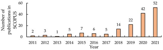
Figure 1.
The growth of low-cost sensors in civil engineering sector.
Figure 1 shows that, from 2011 to 2017, the quantity of the publications associated with the use of low-cost sensors for structural monitoring is negligible (18.2%) and more than 81% of the found articles have been published in the last 4 years (from 2018 to 2021).
To further develop structural system identification methods, standard deviation and distribution functions for measurement devices are required in modeling theoretically physical models. However, these values are usually estimated since researchers who are experts in the analytical analysis may not have access to experimental databases [,,]. This paper studies various distance sensors. Then, through laboratory experiments, this study provides standard deviation and distribution functions for different range distance estimations in various ambient scenarios for several distance sensors.
Distance sensors are typically categorized based on their measuring method. The most widely recognized types include:
- Ultrasonic sensors: These sensors, also known as sonar sensors, are among the most common distance measuring tools. They detect their distance from the target by emitting high-frequency ultrasonic waves. Then, the wave hits any object within the ultrasonic sensor range, bounces off it, and reflects the signal toward the sensor. The sensor calculates the distance by using the time of wave travel and the speed of the signal []. Figure 2 shows the performance of an ultrasonic sensor.
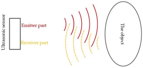 Figure 2. The principle behind distance measurement with sonar sensors.
Ultrasonic measuring tools are not affected by the color or transparency of the object. Furthermore, these sensors are not affected by the brightness of their ambient environment. However, they cannot measure the distance of objects with a complex surface (such as a sponge). Additionally, since the speed of sound is sensitive to humidity and temperature, this sensor is usually coupled with humidity and thermometer sensors to make ultrasonic sensors more accurate [].
- 2.
- Infrared (IR) sensors: These sensors usually measure the distance from an object by emitting infrared light signals and calculating the angle of reflection through triangulation []. When the infrared Light Emitting Diode (LED) emits a beam of light on an object, that light reflects in all directions. A proximity sensor positioned next to the infrared emitter acquires the reflected light waves. The proximity sensor then estimates its distance from the object under study from the angle of the received signal []. Figure 3 illustrates the performance of an IR sensor.
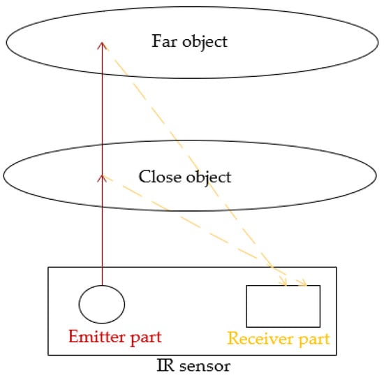 Figure 3. The triangulation procedure of IR sensor.
In Figure 3, the infrared LED puts a beam of light on a particular point of a proximate object. Then, the light signal reflects off the object and reaches the proximity sensor at a certain angle. The proximity sensor estimates the distance mathematically using these data.
- 3.
- Light Detection and Ranging (LiDAR) sensors: The performance of LiDAR sensors is a combination of the ultrasonic and IR sensor processes. For measuring a distance of an object, the transmitter part of the LiDAR emits a laser beam on the target. Then, the receiver part of the LiDAR receives the reflected light signal from the target object. Finally, the distance of the object under study is calculated by multiplying the travel duration of the laser signal and the constant speed of light in the air []. This method has the highest accuracy (such as 0.005% of their final range []) among the techniques discussed above and can detect the distance of small objects []. However, these sensors are expensive (up to EUR 4700 []) and some of them can be harmful to bare eyes []. Even the datasheet for low-cost LiDAR sensors that use class 1 lasers advises users to avoid looking into the laser beam while operating the device [].
- 4.
- LED time-of-flight (ToF) sensors: These sensors fall under the broad LiDAR spectrum and use the time-of-flight methodology to measure distances. ToF sensors use short pulses of light and measure the time between emitted and received signals [,,].
Table 1 compares several widely recognized low-cost sensors based on the technologies mentioned above. The data are organized in the following columns: (1) sensor name; (2) sensor type; (3) reading frequency—sampling frequency speed of the sensor; (4) distance range—the indicated range by the sensor datasheet; (5) dimension; (6) limitations— the limitation of the system such as sensitivity to objects with a complex surface (such as a sponge); (7) input voltage; and (8) price—VAT excluded.

Table 1.
Specifications of different distance sensors.
An analysis of Table 1 shows that despite the low price of the HC-SR04, it has a better reading range and faster data sampling than the GP2Y0A21YK0F sensor. In addition, HC-SR04 is the only sensor in Table 1 whose calculation cannot affect ambient light. However, the datasheet for this sensor noted that the distance estimation is not accurate for objects with an area range smaller than 0.5 square meters or complex surfaces []. Further analysis of Table 1 illustrates that the Lite V3 sensor has the most extensive measuring range. It is also the most expensive sensor under review in this paper. On the datasheet, it mentioned that even though this device uses laser class 1, users should not look at the laser beam [].
The sensors discussed in this section are among the most popular ones currently used in different industry programs [,,,]. Therefore, it is valuable to introduce the latest trends in the distance measuring systems found in the literature.
Terrestrial laser scanning (TLS) is a proposed approach for contactless distance measuring applications. Park et al. developed a new laser scanning measurement technology []. That research used a LiDAR system to assess the health of a structure. The sensor is placed within a distance of 350 m.
Another recent breakthrough in sensor advancement is using an Unmanned Aerial System (UAS) equipped with a commercial-grade video camera to measure a structure’s displacements. However, the error of this approach can be significant in cases where the structure under study experiences a sizeable out-of-plane displacement [].
Recently, the US rail bridge inspection manuals proposed a noncontact displacement measuring system for railroad inspections []. This system is a sensor fusion of a camera and a laser. The camera used in the system corrects the translation and rotation of the laser during its measurements. This new methodology can acquire the dynamic movement of the structure, which a laser or camera alone cannot collect. The experimental test showed up to 20% error, which can decrease with further development of this method.
Miyashita et al. presented a vital literature review on vibration measurements using a Laser Doppler Vibrometer (LDV) and MEMS-based technologies []. This paper describes various noncontact distance measuring tools for bridges. Furthermore, it presents a custom-made triaxle accelerometer with a sampling frequency of 100 Hz used on the experimental analysis of a bridge.
Bhowmick et al. presented a novel method for accurate continuous movement measurement of a one-dimensional vibrating beam using video recording []. This paper uses the camera of an iPhone SE in slow-motion mode. The Root Mean Square (RMS) difference of measurements of a vibrating beam using a commercial LDV sensor and the phone camera is about 0.4 mm. The authors illustrated the first three mode shape evaluation of a two-story scaled structure using this technique []. It is noted that this type of distance measurement imposes some challenges (such as data storage and transmission). They discussed and solved these issues by the proposed method using reconstructed full-field Lagrangian displacement response [].
A paper addressing the status monitoring of tall structures describes a fusion of a Terrestrial Laser Scanner (TLS) and a Ground-Based Real Aperture Radar (GB-RAR). This system can provide the Eigen frequencies and oscillation amplitudes of high-rise structures such as wind towers. The comparison of numerical and experimental analysis using TLS and GB-RAR system fusion shows a precision displacement measurement with about 5 mm of error. Thus, this system is beneficial for noncontact distance measurements and the dynamic behavior of the structure under study [].
On the contrary, VL53l0X VL53l1X (ToF tech) sensors typically use harmless light emission for the bare eyes and provide a high reading frequency at an affordable price. Therefore, by considering the advantages and disadvantages of various sensors, HC-SR04, VL53L0X, and VL53L1X technologies have been selected for the experiments of this paper because of their price, range, eye safety, and sampling frequency. All the sensors listed in Table 1 can be connected to low-cost microcontrollers such as an Arduino.
It is essential to mention that currently, many researchers are using Field Programmable Gate Array (FPGA) circuits instead of microcontrollers (such as Arduino) and minicomputers (such as Raspberry Pi) []. FPGA is a programmable semiconductor integrated circuit in which the majority of its electrical functionality is configurable even after the chipset production [,]. On the one hand, the function ability of microcontrollers (such as Arduino) is like a normal CPU. A code is written in a programming language that gets compiled to machine code. Then, this machine code gets executed by the processor one line at a time.
On the other hand, the configurable logic cells of FPGA make it more versatile, faster and optimizable. However, designing a system based on FPGA is more complex. In addition, indicated by many scholars (such as []), the coding language of Arduino (C programming) is less complicated than that of FPGA (Verilog).
Low-cost microcontrollers can control many low-cost sensors. Arduino is an incredibly cheap microcontroller that is easy to use and based on an open-source electronic prototyping platform with a highly active online community. In fact, many great circuit producers (such as SparkFun Electronics) sell their sensors with open-source Arduino libraries and examples. The sensors are usually connected to Arduino through four methods:
(1) Digital pins: these pins can be configured to function as either input or output.
(2) Analog pins: the primary function of these pins is to read analog sensor data and return integers between 0 and 1023 with 10-bit resolution. Additionally, analog pins can be configured and used like the digital pins and function as either input or output, as well.
(3) Integrated Circuit Bus (I2C): serial data exchange between specialized integrated circuits and the microcontroller. Multiplexors are needed for connecting multiple similar sensors to this port [].
(4) Serial Peripheral Interface (SPI): ports synchronous serial data protocol so the microcontroller can communicate with one or more peripheral devices [,].
Today, low-cost sensors based on Arduino devices are getting widespread attention from civil engineers due to their affordable price and the increased possibility of long-term monitoring with reasonable budgets [,,]. However, the most significant drawbacks of low-cost sensors are their resolution and accuracy compared to traditional commercial solutions. To solve this issue for the first time on record, Komarizadehasl et al. [] found that the average result of multiple low-cost sensors aligned in the same place is more accurate, has less noise density, and has a better resolution than the output of a single sensor for measuring an environmental variation or a structural response. To verify this concept, the researchers connected five similar low-cost accelerometers to an Arduino Uno with a multiplexor through an I2C port. The results were compared with commercial accelerometers and show that an increasing number of randomly selected similar sensors working together is always beneficial. However, data acquisition of this paper required a connected laptop for saving the data.
The literature analysis shows that the methodology proposed in this paper has not been examined with low-cost distance sensors. To fill this gap, this paper investigates the benefits of using an increasing amount of distance sensor coupling to improve the accuracy of distance estimation. Additionally, this paper investigates alternative ways of connecting sensors to the Arduino for excluding the multiplexor from the system. This paper validates this idea through distance measurement laboratory experiments in which a number of distance sensors are connected to microcontrollers. Furthermore, to solve the system’s dependency on an attached computer, this paper uses low-cost data acquisition equipment based on a low-cost Linux computer (Raspberry Pi). Raspberry Pi is programmed to receive and manage the microcontroller outputs without any additional connected computer and gives wireless access to the data acquisition process. In addition, this paper provides the standard deviation and distribution functions of the sensors used in the experiments.
Currently, there are many sensor fusion works in the literature [,,,,]. What separates this paper from those works is how this paper uses the combination of identical sensors to increase the accuracy of low-cost sensors. Moreover, this paper presents the impact of a number of sensor combinations on the overall data accuracy for static distance sensors.
For the first time in the literature, this paper presents a device consisting of 25 analog sensors and 50 digital sensors connected to two Arduino microcontrollers for estimating the distance of an object. Platforms for holding ultrasonic and ToF sensors have been printed using a 3D printer to make sure that all the various ranging sensors are the same distance from the object under study. This system uses a programmed Raspberry Pi that can save the outputs of the Arduinos in a text file. This Raspberry Pi serves as a low-cost data acquisition system that can easily connect to the Internet to control the distance device and access the saved estimations wirelessly. This study investigates the beneficial effects of combining the estimations of several similar sensors to improve the overall accuracy.
This paper is organized as follows: First, Section 2 presents the methodology for making a distance measurement device including 25 of each type of sensors (L530LX, VL53L1X, and HC-SR04). Section 3 describes the characteristics of the performed laboratory experiments and validates the benefits of combining sensors. Section 4 discusses the results of the performed experiments. Finally, Section 5 offers a conclusion.
2. Materials and Methods
This section describes the characteristics of the sensors used in the experiment to validate the accuracy improvement of the similar sensor by coupling several together. A device containing 25 VL53L0X, 25 VL53L1X, and 25 HC-SR04 sensors was constructed to investigate the beneficial effects of averaging the results of multiple distance sensors.
The first subsection of this section introduces the low-cost distance sensors used as measuring devices. The second subsection describes the relations and connections between the microcontrollers, Raspberry Pi, and the sensors. Finally, the third subsection explains the relationship of the sensors to a single solid foundation.
2.1. Low-Cost Distance Sensor
HC-SR04 is a low-cost distance sensor based on the sonar concept methodology with a distance measuring range of 20 to 4000 mm and a resolution of 3 mm. The Arduino interacts with this sensor by digital pin, which is connected to the transmitter and the receiver. For the initiation, the Arduino sends a voltage pulse to the pin, which changes the digital pin from a low to high situation for a moment. This change sends a signal wave through the ultrasonic transmitter. As soon as the signal is sent, the pin status returns to low. When the transmitted signal bounces off of the targeted object toward the sensor’s ultrasonic receiver, the receiver sends a voltage pulse to the digital pin, making it high again. The Arduino estimates the location of the targeted object by multiplying the interval time of the elevated pin by the speed of the sound. Since sound speed depends on ambient temperature and humidity, these data should also be estimated in every ultrasonic distance estimation. When the environmental temperature increases, the kinetic energy of air molecules and the sound velocity increase as well. Sound velocity also has a direct relation to humidity.
To estimate the sound velocity, the temperature and humidity were measured by DHT22. The sound speed is calculated from Equation (1) [].
where sound − velocity and temperature are measured in m/s and degrees Celsius, respectively. Humidity is given in relative terms (%) and shows the ratio of water vapor in the air at a given temperature. Figure 4 shows the ultrasonic, temperature, and humidity sensors.
Sound − velocity = 331.4 + (0.606 × temperature) + (0.0124 × humidity)
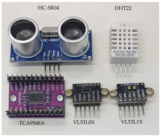
Figure 4.
The used low-cost sensors of the project: HC-SR04 (ultrasonic sensor), DHT22 (temperature and humidity sensor for calibrating the ultrasonic sensor), TCA9548A (multiplexor), VL53L0X (ToF sensor), and VL53L1X (ToF sensor).
Two of the most widely recognized ToF sensors (VL53L0X and VL53L1X) have been used in this project. These sensors have a distance measuring range of 2 and 4 m, respectively, with a 1 mm resolution. VL53L0X and VL53L1X communicate with the Arduino through an I2C communication port. This communication port consists of a Serial Clock Line (SCL) and a Serial Data Line (SDA) pin, which can be connected to various digital sensors (those which have SCL and SDA pins) simultaneously as long as the connected sensors have different addresses. There are two different connection ways to connect a number of ToF sensors to a microcontroller: (1) by default address changing [] or (2) through a multiplexor. Default address changing with VL53L0X and VL53L1X circuits involves using a few lines of code to change their default addresses to other addresses [,] (TCA9548a). A multiplexor connects the sensors with the same address to Arduino. Up to 64 similar sensors can be introduced to the Arduino []. Although the first methodology seems more accessible and cheaper, it is not as reliable or stable as the second method. Moreover, if a ToF sensor in the first method gets damaged, burned, disconnected, or stops working for any reason, the whole system stops working until the problem is solved or the burned sensor is replaced. To improve reliability, this research connected the I2C sensors to the microcontrollers through a multiplexor.
2.2. Microcontroller Section and Data Acquisition
This subsection studies the correct connection of the distance sensors to microcontrollers for data sampling and data acquisition, the number of microcontrollers needed, and microcontroller communication. Data acquisition posed a few challenges, which are detailed here along with their corresponding solutions. (1) Electricity shortage: By using a single Arduino Uno with 75 sensors, the input voltage for the ultrasonic was lower than 3.5 V, which resulted in no measurement estimation from HC-SR04. An Arduino Mega connected to a spread power source was used to fix this issue. The sensors were distributed among these two Arduinos. (2) Single output: The serial communication of Arduino Uno was connected to the Arduino Mega to save data from only one Arduino and have the sensors measuring simultaneously. During the distance measurement, these Arduinos were in touch with each other. First, both Arduinos checked their connected sensors. Second, the Arduino Uno printed a character that ordered the Arduino Mega to activate its connected distance sensors. Third, the Arduino Mega received the character and confirmed with the Arduino Uno by sending a different character. At this moment, both microcontrollers had already forced their connected sensors to measure the distance of the targeted object. The Arduino Uno then printed the values of its sensors in its serial communication and waited for another character from the Arduino mega. When the Arduino Mega was finished with its measurements, it triggered a short delay (making sure that Arduino Uno was finished with its printing and was waiting for Arduino Mega), and it sent the character. Shortly after printing this character, the Arduino Mega sent all of its measurements to the Arduino Uno. Finally, by receiving the Arduino Mega character, Arduino Uno started printing the outputs of the Arduino Mega with a space from its printing. This way, the information was only received from the Arduino Uno. (3) Data acquisition: Raspberry Pi was connected to the master Arduino (Arduino Uno) for saving all the measurements. The Raspberry Pi provided power for the Arduino Uno and acquired its output through a written Python code. (4) Supply: The Raspberry Pi requires input power with 5 V and 2.5 A. Standard adaptors for mobile charging or power-banks only provide 5 V and 2.1 A. Consequently, the Raspberry Pi showed a low-power error that affected the connected Arduino Uno. However, the Arduino Mega can connect to any habitual power bank or micro-USB mobile charger.
2.3. Construction of the Measurement Device
A few steps were taken to make sure that all sensors measured the same distance from the object under study. (1) Sensor base: A PVC plate (Figure 5a) provided a solid, uniform, and smooth base for the sensors. (2) Sensor connection to the PVC plate: Three-dimensional printed clamps were designed to connect the sensors to the plate (Figure 5b). These 3D-printed clamps were developed to hold the HC-SR04, VL53L0X, and VL53L0X at a known height. These clamps were glued to the PVC plate (Figure 5a) and then the sensors were glued to the 3D-printed clamps (Figure 5c). At this position, the measuring part of the ultrasonic sensors (the top of the HC-SR04 sensors) was located at a 25 mm height from the PVC plate. The thickness of the ToF sensors was fixed to 2 mm. These heights were taken into account by implementing these values to the Arduino code. (3) Wiring: The sensors were wired as shown in Figure 5d. The 25 ultrasonic sensors were connected to the digital ports of the microcontrollers, and the 50 sets of ToF sensors were connected to I2C ports of the microcontrollers using multiplexors (Figure 6). (4) The Raspberry Pi was connected to the Arduino Uno for wireless control and saving measurements. Then, the Arduino Uno was connected to the Arduino Mega using two jumper wires (Figure 6). Finally, the Arduino Mega and Raspberry Pi were connected to an external power source. Figure 5e shows the developed distance measuring device in the laboratory. As seen, the device was located on a fixed platform experiment testbed. The mobile part of the actuator is the upper jaw of the jack (Figure 7). In addition, the flowchart of the construction of measurement device is presented in Figure 5f.
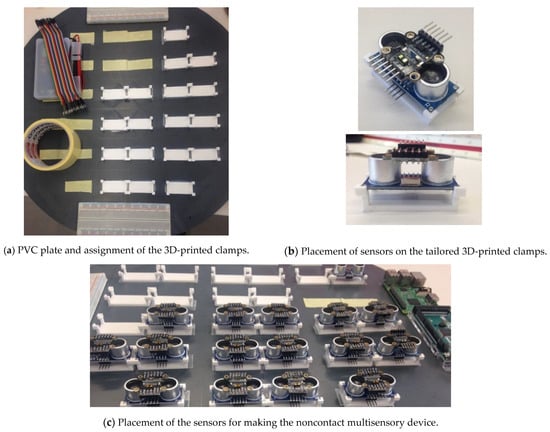
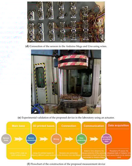
Figure 5.
The components of the distance measuring device: (a) PVC sheet for attaching the sensors and the data acquisition equipment, (b) designed 3D-printed base for holding the various sensors together at a known height, (c) sensor allocation, (d) wiring the system together, (e) the experiment platform for validating the accuracy of several different low-cost sensors and (f) flowchart of the construction of the proposed measurement device.
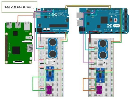
Figure 6.
Scheme of the connections between the microcontrollers and the Raspberry Pi.
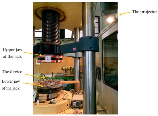
Figure 7.
The laboratory experiment equipment.
In Figure 6 shows all of the assets required to make the multisensor distance measuring device. Figure 6 also displays the serial connection of Arduino Uno and Mega, as drawn by Fritzing software []. Pins 0 (RX) and 1 (TX) on the Arduino Uno are connected to pins 1 (TX) and 0 (RX) on the Arduino Mega, respectively. RX and TX pins stand for receiving and transmitting pins of the Arduino serial communication.
Since this paper targets static sensors, the sensors were not synchronized with microsecond resolution. Even though the ToF sensors have a very high sampling frequency, the ultrasonic sensors need some time to measure data. For that, some delay functions were used in the Arduino code of the tailored device. This system measured distance once every 10 s. In the absence of ultrasonic sensors, ToF sensors could have been synchronized with microsecond resolutions, as in the recently published article by the same authors [].
The current system has already been used with accelerometers, as well. Recently, Komarizadehasl et al. [] published a paper discussing noise reduction of dynamic sensors using several synchronized low-cost accelerometers. Thus, a system made from dynamic sensors can be used for tests with dynamic loadings.
3. The Experiment
This section describes the validation experiments of the multisensor distance measuring device. An experiment at the Structural Laboratory Lluís Agulló of Universitat Poliècnica de Catalunya, Barcelona Tech (Spain) assessed the impact of sensor combination and provided a fair comparison between the introduced ToF and ultrasonic sensors. The jack seen in Figure 7 was used to measure the distance of an object from the distance measuring device. The distance between the machine’s upper and lower jaw can be altered. This jack was selected for this laboratory experiment for three key reasons, as described below. (1) Dimension of target object: The area of its movable part (the upper jaw) is slightly above 0.5 square meters. This made the distance between the two jaws measurable by the HC-SR04 sensors []. (2) Movability: Since the upper jaw of this jack moves, different distances can be measured by the tailored distance measuring device. The distances were calculated by a steel measurement pattern. (3) Ambient light: A projector light was placed on the side of this jack to produce an extremely bright situation for simulating day and night in the laboratory. To show the capability of the proposed device under a noisy environment commonly found in the industry, the experiments were carried out during the active hours of the laboratory. In addition, the projector shown in Figure 7 was used for additional environmental noises.
Ten static tests were carried out on this jack. In every test, the upper jaw of the jack was fixed with a measured distance from the lower jaw by a steel measurement pattern. Every test had a duration of 15 min. Additionally, the distance of the lower jaw from the tip of the sensors was measured for data postprocessing. The lower jaw of the jack was located precisely 60 mm lower than the tip of all sensors mounted on the device.
Each of these ten experiments was performed once with the projector off and once with the projector on. This ambient light simulates the presence and the absence of the sun. In outdoor measurements, there are moments when the sun may be shining directly on the distance-measuring sensors. This work examines the sunlight effect through this laboratory experiment, which this paper refers to as experiments with excessive ambient light. The experiments without ambient light were acquired while the projector in Figure 6 was off. However, the laboratory has a permanent lighting system that could not be turned off during working hours. Table 2 shows a summary of the experimental tests.
Table 2.
Characteristics of the performed tests.
All the tests listed in Table 2 were conducted once with the projector on and once with the projector off. The steel measurement pattern was used to secure the measurements. The numbers refer to the tip of the measuring device’s sensors to the jack’s upper jaw.
4. Result and Discussion
This section describes the experimental results. The first subsection discusses the detected errors of the sensors and proposes a code for data postprocessing. This subsection also presents the average results of all similar sensors. The second subsection shows the beneficial effect of coupling similar sensors by comparing the results of a random sensor with the fused results of 25 similar sensors. Finally, the third subsection presents the increasing accuracy of devices with a higher number of similar coupled sensors. This investigation was conducted by comparing combinations of connected similar sensors with the benchmark measurements. The results show that all other varieties of the selected sensors have higher accuracy than the values presented in this paper.
4.1. Error Recognition
Some ultrasonic and ToF sensors reported an error during certain tests and their data were excluded from the postprocess data. These errors can be categorized into two types:
(1) Ultrasonic errors: Since the further inspection of the measuring device showed no faulty connections and no problem with the uploaded code, it was concluded that the flow of the electricity was causing issues in random sensors during some of the experiments. The ToF sensors draw more current from the device when they estimate the distance of an object which is located further away. Drawing more current from a multisensor device within a constant 400 mA current output (200 mA each Arduino []) resulted in a voltage drop. As already mentioned, the HC-SR04 could not work with a current lower than 3.6 V. The sensors indicated an error by either printing “0” or printing a value smaller than the actual distance. Unlike ToF sensors, ultrasonic sensors are low-frequency sensors with steady outputs. By plotting the results of ultrasonic sensors and studying them, these outliers are approximately 10% smaller than the estimated value. These values have been considered faulty values as well and have been excluded from the outputs. Figure 8 shows an example of this error.
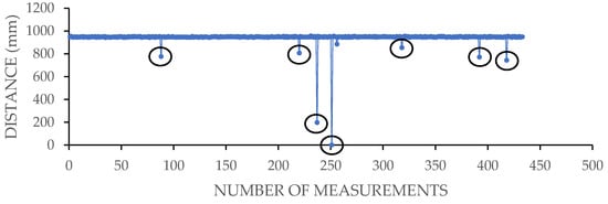
Figure 8.
Excluding the outliers of HC-SR04 estimations.
(2) ToF sensors: These sensors are sensitive to ambient light. Whenever a robust environmental light beam was focused on a sensor, the sensor was printing an error coded as “8190” instead of the measured distance. In addition, this type of sensor will print a coded value of “65,535” if it is burned, has a faulty connection, or the input power is not enough.
To address the issues above, a code was used to exclude the faulty readings. This code first extracts the acquired HC-SR04, VL53L0X, and VL53L1X sensor data from the Raspberry Pi output in three different matrixes. In each matrix, the columns specify a given sensor and each row is a measurement cycle. Second, the code excludes the rows in which at least one of its values is faulty. Incorrect values are the coded errors mentioned above, including: 0, 8190, and 65,535.
Table 3 displays the average results of all similar sensors with their standard deviations (STDEV) for each experiment with excessive ambient light (such as VL53L1X Light) and without it (such as VL53L1X). The first column lists the distance of the sensors from the targeted object, as measured by a steel measurement pattern. The column average then represents the average results of 25 distance sensors for 80 measurement cycles. The STDEV column represents the standard deviation of the same distance sensors on average for 80 data acquisition cycles in each experiment. The columns with no information show the incapability of distance measurement by the sensor type.
Table 3.
The normalized values of similar sensors.
Table 3 shows that ultrasonic sensors can measure higher distances more accurately. Moreover, ToF sensors decrease in accuracy as their distance from the target object increases. Further analysis of Table 3 shows that the standard deviation of all sensors in all situations rises with the increment of the object distance. Ambient light results in lower accuracy for ToF sensors and produces a more significant standard deviation. ToF sensors are also more sensitive to ambient light at larger distances. Table 3 also shows that even though VL53L0X measured distances up to 68 cm in the absence of the projector light, it only measured distances up to 48 cm when the projector light was on. VL53L0X sensors were also affected by ambient light. Subsequently, the VL53L0X can be introduced as the least effective distance sensor in this experiment due to its short distance range. This higher data fluctuation results in a significant standard deviation ratio and incorrect calibration. HC-SR04 and VL53L1x report very similar results on short distances, which demonstrates their accurate company calibration. For distances greater than 450 mm, the difference between the results of the ultrasonic sensor and VL53L1X is more than 3 mm. Another interesting result from the analysis of this table is the effect of the projector light on VL53L1X. This sensor measured a higher distance from the estimations of the HC-SR04 and the steel measurement pattern measurements when the projector was on.
Errors of faulty sensors can easily affect the overall performance of data acquisition. Consequently, errors should be removed in postprocessing evaluations. If a sensor shows dissonance among other ones, the data output of the faulty sensor or sensors should be deleted and the sensor replaced. During long-term monitoring, when the health status of a sensor that is a part of the sensor combination is suspicious, the data of that sensor can be removed. The overall accuracy and resolution are decreased by removing a sensor from the sensor combination, but the system still works at a lower resolution until the faulty part is replaced. If a traditional single sensor is used for the same purpose, however, its health status is unlikely to be evaluated because there is no other sensor to compare to its results. In such cases, no data can be acquired until the traditional sensor is identified and replaced.
4.2. Beneficial Effect of Combining Similar Sensors
This subsection investigates the benefit of coupling all the sensors of a similar type. Figure 7 illustrate the filtered results for a single experiment for 25 sets of VL53L0X, 25 sets of VL53L1X, and 25 sets of HC-SR04 in the absence of excessive ambient light with the targeted object exactly 29 cm away, respectively. In these figures, the vertical axes represent the distance of the jack’s upper jaw from the device, as measured by the sensors. The horizontal axes indicate the number of measurement cycles. In every Figure, 25 different colors show the measurements of the 25 sensors of each type.
Analysis of Figure 9 shows the fluctuation of acquired data by various distance measuring technologies. VL53L0X has higher data fluctuation and sensitivity to the environmental situation than the other sensor types. VL53L1X shows more stable results. For example, although data acquisition by VL53L0X shows 90 mm of data fluctuation, VL53L1X shows less than 40 mm. Figure 9 also shows that HC-SR04 has the most stable data report among the selected distance measuring sensors. In fact, HC-SR04 has less than 6 mm of data fluctuation. The standard deviation of a single VL53L0X, VL53L1X, and HC-SR04 sensor from Figure 9 was on average about 7.3, 5.1, and 0.9, respectively.
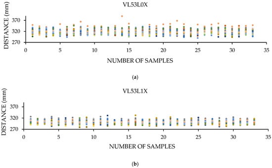
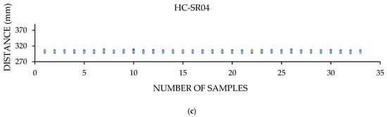
Figure 9.
Filtered output of distance sensors for an experiment: (a) results of VL53L0X, (b) results of VL53L1X, and (c) results of HC-SR04.
The results of all 25 sensors for each cycle have been averaged to illustrate the benefit of the sensor combination. Figure 10 illustrates the results of this development. The orange line is the measurement carried out by a steel measurement pattern.
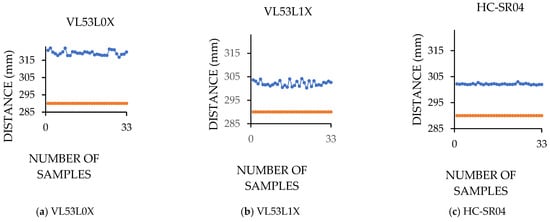
Figure 10.
Combined outputs of similar sensors.
Analysis of Figure 10 shows the benefit of using the averaged results of 25 sensors for measuring a distance instead of using the results of a single sensor. The fluctuation of VL53L0X data decreased to 7 mm, which is 12 times less fluctuation. The fluctuation of VL53L1X and HC-SR04 was reduced to approximately 4 mm and 1 mm, respectively. The standard deviation of 25 fused VL53L0X, 25 fused VL53L1X, and 25 fused HC-SR04 sensors was 1.3, 1.1, and 0.2, respectively. The combing sensors significantly improved noise-canceling and graph smoothing, as well. Each sensor has inherent noises different from the other similar sensors. By averaging the results of multiple sensors, these noises either get smaller or are canceled altogether. The randomness of these noises has been investigated through a few experimental tests (citing conference papers). Further analyses of Table 3 and Figure 10 show the potential bias associated with the incorrect or lack of calibration of individual sensors. In fact, the offset of the VL53L0X sensor from the steel measurement pattern measurements is about two centimeters. Additional calibration of this sensor is needed for sensitive measurements.
4.3. Effect of Coupled Similar Sensors
This subsection investigates the beneficial impacts of adding an increasing number of fused sensors in detail.
Error measurements were calculated by a steel measurement pattern to compare all sensors (see Table 3). A combinatory program written in MATLAB found the least effective sensor combination for each experiment. This code first opens all the documents related to filtered outputs of similar sensors for all the experiments. Second, the code generates various sensor combination probabilities for the 25 sensors. Since the server computer used for this experiment could not calculate more than eight fused sensor combinations, this study’s most effective fused sensor combination is eight. Even though 25 similar sensors were mounted on the distance sensing device in this work, only up to eight sensors were used for the combinatory analysis. Experimental tests show no significant improvement as of eight combined sensors. Figure 11 shows the maximum possible error for every sensor combination for different experiments with different distances.
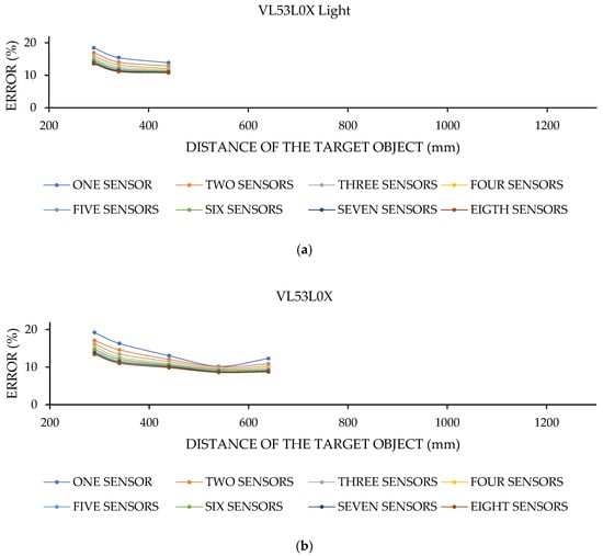
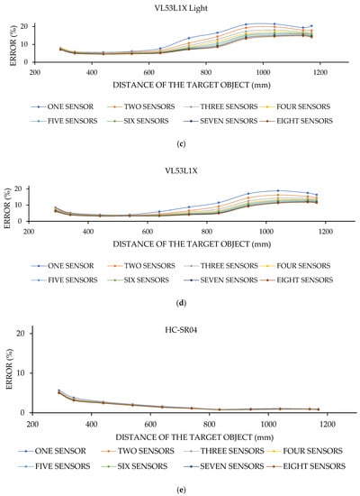
Figure 11.
Comparing the worst-case sensor combination with different distance measurement technologies: (a) VL53L0X distance estimations affected by an excessive light source, (b) VL53L0X distance estimations in darkness, (c) VL53L1X distance estimations affected by an excessive light source, (d) VL53L1X distance estimations in darkness, and (e) HC-SR04 distance measurements.
Analyses of Figure 10a,b reveal the limited distance range of VL53L0X for experiments with and without ambient light. Despite the high errors associated with this type of sensor when used alone, the error decreases with and without ambient light when multiple sensors are fused together. Even though the results of a single sensor in the worst-case scenario are 19% in the absence of ambient light, the exact measurement with eight fused sensors shows only 13% error, which confirms the benefit of combining sensors. This sensor is more accurate for intermediate ranges but does not work very well for very close or very far distances. Its lowest error appears when measuring a distance of 54 cm regardless of the number of fused sensors or the ambient light situation. The most significant effect of the sensor combination is seen with three VL53L0X sensors coupled together.
Figure 9c,d detail the outputs of VL53L1X for experiments with and without ambient light. This sensor offers a broader range and more minor errors than VL53L0X. Like VL53L0X, this sensor works better for intermediate distances. These figures show how combining sensors reduces the overall estimation errors for both experiments with and without the ambient light. Figure 11d shows that the worst-case estimation error scenario for a single sensor is 9%.
In contrast, the worst-case combination of eight fused sensors has an estimation error of 4% in the same experiment. This sensor, like the VL53L0X, estimates distance in an intermediate range. However, the medium range of VL53L1X is more significant and is between 34 cm and 64 cm.
The combinatory analysis of Figure 11c shows that, while the error of a single VL53L1X in the worst-case scenario is between 5% and 22%, when coupling eight sensors, the error range in the worst-case combination of the chosen sensors is between 4% and 15% when the projector is on. The highest and lowest error for a single sensor in the absence of high ambient light is between 4% and 18%, and by combining eight sensors, that range becomes 3% to 12%. The error continues to lower more with a higher number of combined sensors. The most significant effect of sensor coupling for VL53L1X is observed with at least four averaged sensors.
Figure 11e shows the high accuracy and low data fluctuation of the HC-SR04 sensor, although combining sensors increases the accuracy and describes the estimation error. Analysis of Figure 11e shows that the effect of sensor combination is not as evident for HC-SR04 sensors when compared to ToF sensors. However, carefully studying the performance of HC-SR04 sensors shows their improving accuracy with distance increment. The most significant impact of the sensor combination is observed in the experiment when the target object is at a distance of 29 cm. In that experiment, the error of a single sensor in the worst-case scenario improves from 6.7% to 5.9%, with eight ultrasonic sensors fused in selecting the worst-case combination.
Further analysis of Figure 11 shows that the sensor combination improves the estimation accuracy of VL53L0X and VL53L1X sensors more than that of the HC-SR04. ToF sensors (such as VL53L0X and VL53L1X) are known to experience more noises than ultrasonic (such as HC-SR04) sensors. Consequently, the data acquisition of ToF sensors is usually postprocessed for noise reduction and signal improvement []. Averaging the results of a number of similar sensors helps to reduce individual noises or imperfections of the used sensors. Since ToF sensors are influenced by more environmental parameters (color, material, distance, and lighting), their combination shows a more significant accuracy improvement than ultrasonic sensors that are only affected by fewer environmental parameters (such as temperature).
Most improvement occurs when at least two sensors are combined. In such cases, the overall error for the worst-case scenario is 6.33%. Even though the error from combining eight VL53L1X for all experiments in the absence of ambient light was between 3% and 12%, a single HC-SR04 reports errors between 1% and 7%, which is very low. Here, the precision of a single ultrasonic sensor for the distance measurement of semi-controlled laboratory experiments is higher than eight fused VL53L1X sensors. The price of a single VL53L1X is about five times more than that of a single HC-SR04. As a result, the low cost of HC-SR04 makes it the best candidate for sensor combination applications.
This work presents a way of improving the accuracy of low-cost sensors without postprocessing or manipulating the outputs. In the current form, a device made from only ultrasonic sensor combinations can be used in different locations of a dam to measure the approximate water level. The device is not currently tailored to be used in the industry. This device contains 75 sensors (analog and digital) with a radius of 250 mm, which is used to research and analyze the impact of combining similar sensors. The results of this paper can be used further in making tailored devices with an acceptable range of accuracy for a known ambient situation. For example, in a dark place with a measuring range of 540 mm, two combined Vl53l1x have up to 3.7% error. The size of a device made from these two sensors would be 26 × 8 × 2 mm. The price and size of any sensor combination can be calculated from the data available in Table 1.
It is essential to mention that combining commercial circuits will oversize the final product. To reduce this enlargement, the Printed Circuit Board (PCB) of the sensor can be redesigned for specific measuring purposes. Therefore, the proposed device of this paper with the current resolution is suitable for remote liquid level detection where the size of the object under study (water level) is large enough for the oversized device made from sensor combination. In civil engineering, this level detection is commonly used for imposed load calculation of dams [] and safety and water level of open and closed canals [] and bridges [].
4.4. Statistical Evaluation
This subsection presents the distribution function of the sensors for every test. It is essential for every researcher who works on structural system identification methods to model measurement data in their research. As indicated by many scholars (such as those of [,]), these standard deviation functions are usually assumed without being measured. This section can further enrich the current literature with actual data by proving the standard deviation functions of various noncontact distance sensors in different ambient situations. These functions can help advance structural system identification applications and noise-canceling functions without learning the required electronic engineering skills for setting up low-cost distance sensors.
In order to show an overall distribution of each type of sensor for each performed laboratory experiment, the normal distribution function for averaged results for each kind of sensor (like the data in Figure 9) was calculated in Excel. The normal distribution check of the estimated data as then calculated through SPSS software using the Shapiro–Wilk p-value and Kurtosis Z-value methods. Many scholars indicate that a distribution is normal as long as the Z-value is +/− 1.96 and the p-value is higher than 0.05.
Figure 12, Figure 13, Figure 14, Figure 15 and Figure 16 show the normal distribution functions for VL53L0X, VL53L1X, and HC-SR04 sensors for all of the experiments presented in this study. The horizontal axes of all graphs are the averaged estimated data of all sensors in millimeters, and the vertical axes are the normal distribution function. Table 4, Table 5, Table 6, Table 7 and Table 8 investigate the normal distribution of the estimation.
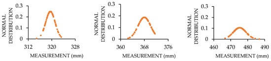
Figure 12.
The normal distribution function of VL53L0X for tests with ambient light.
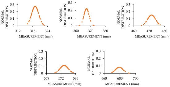
Figure 13.
The normal distribution function of VL53L0X for tests with no excessive ambient light.
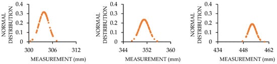
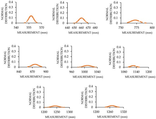
Figure 14.
The normal distribution function of VL53L1X for tests with ambient light.
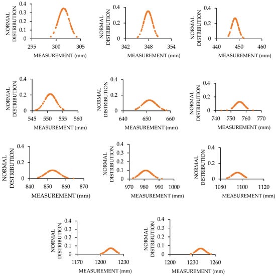
Figure 15.
The normal distribution function of VL53L1X for tests with no excessive ambient light.
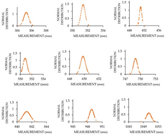
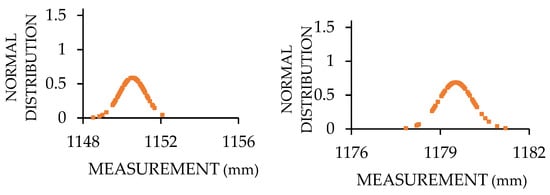
Figure 16.
The normal distribution function of HC-SR04 for various distance measurements.
Table 4.
Statistical analysis of VL53L0X for tests with ambient light.
Table 5.
Statistical analysis of VL53L0X for tests with no excessive ambient light.
Table 6.
Statistical analysis of VL53L1X for tests with ambient light.
Table 7.
Statistical analysis of VL53L1X for tests with no excessive ambient light.
Table 8.
Statistical analysis of HC-SR04 values (those written in red do not follow the normal distribution).
Analyzing Figure 12, Figure 13, Figure 14 and Figure 15 shows that the distribution function value for ToF sensors decreases when the target object is located further away from the distance sensor. The area under the graph increases with the target object locating further away. The presence of ambient light makes this area even bigger. These indicators mean that the probability of estimating the right answer by the ToF sensors decreases as the distance increases, or when ambient light exists.
Careful inspection of Table 4, Table 5, Table 6 and Table 7 illustrates that the distributions of VL53L0X and VL53L1X in both the presence and absence of excessive ambient light are normal.
Analysis of Figure 16 shows that some of the distributions are not following the regular pattern. In fact, the information in Table 8 helps us check the normal distribution of HC-SR04 outputs for the performed laboratory experiments.
Analysis of Table 8 shows that most of the estimations follow a normal distribution. In fact, the assessments that are not following normal distribution may appear because of the lack of electrical current necessary for the sensors to perform accurately.
Table 9 shows the price of devices made from combining similar sensors for an experimental test. In this test, sensors have estimated a distance of 540 mm in the absence of excessive ambient light.
Table 9.
Price comparison of the devices made from coupled sensors.
Analysis of Table 9 shows that the accuracy of Vl53l0X is so low that even after combining eight sensors, the error is still higher than that of Vl53l1X and HC-SR04. In fact, by using only two Vl53l1X sensors, the benefits of sensor combinations, such as a smoother standard deviation and having a backup sensor in case one sensor is faulty, can be reached with a lower price. The ultrasonic sensor has the highest accuracy, but it cannot be used in places with high ambient temperature variations. A commercial noncontact distance sensor acquisition resolution is extracted from its datasheet to show the cost efficiency of the systems in this study. O1D100 in the distance range of 200 mm to 1000 mm has an 18 mm accuracy (1.8%). The price of O1D100 is EUR 383 [].
Further analysis of Table 9 suggests no need to combine 25 similar sensors to improve the accuracy of data acquisition. By using two combined HC-SR04 sensors, the estimation error will be less than two percent. The same number of combined VL53L1x sensors will also result in accurate distance estimation. In fact, based on the required sensitivity, more sensors can be combined. The final number of sensor combinations depends on some variables such as the size of the object under study and its movements.
5. Conclusions
The standard deviation and distribution functions of different sensors are needed to develop structural system identification methods further. Many low-cost sensors have such low resolutions that their use has been exempt in civil engineering applications with low budgets. As a result, justifying the use of low-cost sensors in civil engineering requires improvements in both deep noise canceling and accuracy.
This paper’s main contribution and novelty are to combine the results of similar sensors for mitigating the adverse effects of environmental or individual inherent noises of low-cost sensors for estimating static environmental variations. The study finds that by coupling a number of similar sensors for measuring the same structural response or variation, the overall accuracy is higher than the estimation of an individual sensor. This paper also contributes to the civil engineering literature by providing the standard deviation and distribution functions of these types of sensors for different environmental circumstances. It is noted that the developed noncontact distance measurement device of this paper is intended to be used for water level control of dams, bridges, and open canal applications.
To investigate the proposed methodology, this paper uses 75 various distance sensors mounted on a stiff foundation with 3D-printed bases. These sensors (25 HC-SR04, 25 VL53L0X, and 25 VL53L1X) were connected to two microcontrollers. The microcontrollers were connected through transmission and receiving ports (RX and TX ports) of the microcontroller serial communication gates. Data acquisition was carried out using a Raspberry Pi connected to one of the microcontrollers. The acquired data were then uploaded to the cloud.
The analysis of the acquired data shows that sensor combination is beneficial for both analog and digital sensors, regardless of the ambient light situation. The combination of 25 similar sensors showed a considerable improvement in estimation accuracy and data fluctuation for all sensor types. It is also shown that even the worst combination of sensors has a lower error than the estimation of the worst selected sensor. Further analysis of the data shows that HC-SR04 is a cheap analog distance sensor and has higher estimation accuracy than the expensive time-of-flight (ToF) sensors (VL53L0X and VL53L1X) in laboratory experiments carried out in a civil engineering laboratory with and without excessive ambient light. Moreover, the lower price of HC-SR04 compared with the other ToF sensors in this study can justify the sensor combination methodology for this type of sensor.
The significant endowments and limitations of the proposed measuring distance device through combining estimations of several similar sensors can be summarized as follows.
Combining the results of multiple similar ranging sensors improves the estimation accuracy by averaging the responses of uncalibrated sensors. By comparing the measurement of individual sensors with the combined results of a few sensors, the sensitivity and accuracy of individual sensors can be monitored for the duration of the data acquisition process. In the case of a single malfunctioning sensor, the acquisition process can continue due to several combined sensors instead of using the outputs of a single measuring tool. Furthermore, since not all monitoring applications require a high level of accuracy, such as the water level monitoring of dams, low-cost sensors can be combined to make a low-budget ranging device for these applications. Finally, with the open source and open hardware of the proposed measuring device, changes can be applied efficiently.
The adverse effects of ambient light on ToF sensors were not amended significantly through a similar sensor combination. This issue needs to be studied by combining ToF sensors’ estimations with ultrasonic sensors that are not affected by excessive light in the environment. Furthermore, the use of ToF sensors in this system has an indirect relation with the luminous response of a light detector sensor. More precise instruments, such as Linear Variable Differential Transformer (LDVT) sensors, are needed to perform the distance measuring experiments more accurately. Finally, individual sensor responses must be postprocessed to remove the proposed system’s inherent noises.
Author Contributions
Conceptualization, J.T. and J.-A.L.-G.; methodology, S.K.; software, B.M.; validation, S.K. and J.T.; formal analysis, S.K.; investigation, J.T.; resources, H.M.; data curation, B.M.; writing—original draft preparation, S.K.; writing—review and editing, S.K.; visualization, J.-A.L.-G.; supervision, J.T.; project administration, H.M.; funding acquisition, J.T. All authors have read and agreed to the published version of the manuscript.
Funding
The Spanish Ministry of Economy and Competitiveness and Feder Funds: BIA2017-86811-C2-1-R; the Spanish Ministry of Economy and Competitiveness and Feder funds: BIA2017-86811-C2-2-R; the Secretaria d’ Universitats i Recerca de la Generalitat de Catalunya, Catalunya, Spain: 2017 SGR 1482; Spanish Agencia Estatal de Investigación del Ministerio de Ciencia Innovación y Universidades and Fondo Social Europeo: PRE2018-083238.
Institutional Review Board Statement
Not applicable.
Informed Consent Statement
Not applicable.
Data Availability Statement
All data and results are presented in this paper.
Acknowledgments
The authors are indebted to the Spanish Ministry of Economy and Competitiveness for the funding provided through the research project BIA2017-86811-C2-1-R, directed by José Turmo, and BIA2017-86811-C2-2-R, directed by Jose Antonio Lozano-Galant. All these projects are funded with FEDER funds. Authors are also indebted to the Secretaria d’ Universitats i Recerca de la Generalitat de Catalunya, Catalunya, Spain for the funding provided through Agaur (2017 SGR 1482). It is also to be noted that funding for this research has been provided for Seyedmilad Komarizadehasl by the Spanish Agencia Estatal de Investigación del Ministerio de Ciencia Innovación y Universidades grant and the Fondo Social Europeo grant (PRE2018-083238).
Conflicts of Interest
The authors declare no conflict of interest.
References
- Bilro, L.; Alberto, N.; Pinto, J.L.; Nogueira, R. Optical Sensors Based on Plastic Fibers. Sensors 2012, 12, 12184–12207. [Google Scholar] [CrossRef] [PubMed] [Green Version]
- Barrias, A.; Casas, J.R.; Villalba, S. A Review of Distributed Optical Fiber Sensors for Civil Engineering Applications. Sensors 2016, 16, 748. [Google Scholar] [CrossRef] [Green Version]
- Mobaraki, B.; Lozano-Galant, F.; Soriano, R.P.; Pascual, F.J.C. Application of Low-Cost Sensors for Building Monitoring: A Systematic Literature Review. Buildings 2021, 11, 336. [Google Scholar] [CrossRef]
- Rodrigues, D.V.Q.; Li, C. A Review on Low-Cost Microwave Doppler Radar Systems for Structural Health Monitoring. Sensors 2021, 21, 2612. [Google Scholar] [CrossRef] [PubMed]
- Kohler, M.D.; Heaton, T.H.; Cheng, M.H.; Singh, P. Structural health monitoring through dense instrumentation by community participants: The community seismic network and quake-catcher network. In Proceedings of the 10NCEE, Anchorage, AK, USA, 21–25 July 2014; pp. 21–25. [Google Scholar] [CrossRef]
- Simkin, G.; Beskhyroun, S.; Ma, Q.; Wotherspoon, L.; Ingham, J. Measured response of instrumented buildings during the 2013 Cook Strait earthquake sequence. Bull. N. Z. Soc. Earthq. Eng. 2015, 48, 223–234. [Google Scholar] [CrossRef]
- Lynch, J.P.; Wang, Y.; Swartz, R.A.; Lu, K.C.; Loh, C.H. Implementation of a closed-loop structural control system using wireless sensor networks. Struct. Control Health Monit. 2008, 15, 518–539. [Google Scholar] [CrossRef]
- Soriano, R.P.; Mobaraki, B.; Lozano-Galant, J.A.; Sanchez-Cambronero, S.; Muñoz, F.P.; Gutierrez, J.J.; Soriano, R.P.; Mobaraki, B.; Lozano-Galant, J.A.; Sanchez-Cambronero, S.; et al. New Image Recognition Technique for Intuitive Understanding in Class of the Dynamic Response of High-Rise Buildings. Sustainability 2021, 13, 3695. [Google Scholar] [CrossRef]
- Komarizadehasl, S.; Khanmohammadi, M. Novel plastic hinge modification factors for damaged RC shear walls with bending performance. Adv. Concr. Constr. 2021, 12, 355–365. [Google Scholar] [CrossRef]
- Orlano, P. Geomatic techniques for the colonnade structural analysis of the historical “chiaramonte steri” building. Int. Arch. Photogramm. Remote Sens. Spatial Inf. Sci. 2019, 42, 923–928. [Google Scholar] [CrossRef] [Green Version]
- Aygun, L.E.; Kumar, V.; Weaver, C.; Gerber, M.; Wagner, S.; Verma, N.; Glisic, B.; Sturm, J.C. Large-Area Resistive Strain Sensing Sheet for Structural Health Monitoring. Sensors 2020, 20, 1386. [Google Scholar] [CrossRef] [Green Version]
- Caponero, M.A.; Dell’Erba, D.; Kropp, C. Use of fibre optic sensors for structural monitoring of temporary emergency reinforcements of the church S. Maria delle Grazie in Accumoli. J. Civ. Struct. Health Monit. 2019, 9, 353–360. [Google Scholar] [CrossRef]
- Peng, T.; Nogal, M.; Casas, J.R.; Turmo, J. Role of sensors in error propagation with the dynamic constrained observability method. Sensors 2021, 21, 2918. [Google Scholar] [CrossRef] [PubMed]
- Lei, J.; Lozano-Galant, J.A.; Nogal, M.; Xu, D.; Turmo, J. Analysis of measurement and simulation errors in structural system identification by observability techniques. Struct. Control Health Monit. 2017, 24, 1–21. [Google Scholar] [CrossRef]
- Lei, J.; Lozano-Galant, J.A.; Xu, D.; Turmo, J. Structural system identification by measurement error-minimizing observability method. Struct. Control Health Monit. 2019, 26, e2425–e2444. [Google Scholar] [CrossRef]
- Yang, L.; Feng, X.; Zhang, J.; Shu, X. Multi-Ray Modeling of Ultrasonic Sensors and Application for Micro-UAV Localization in Indoor Environments. Sensors 2019, 19, 1770. [Google Scholar] [CrossRef] [PubMed] [Green Version]
- Komarizadehasl, S.; Turmo, J.; Mobaraki, B.; Lozano-galant, J.A. Comparison of different low-cost sensors for structural health monitoring. In Bridge Maintenance, Safety, Management, Life-Cycle Sustainability and Innovations; CRC Press: Boca Raton, FL, USA, 2021; pp. 186–191. [Google Scholar] [CrossRef]
- Dong, Z.; Sun, X.; Liu, W.; Yang, H. Measurement of free-form curved surfaces using laser triangulation. Sensors 2018, 18, 3527. [Google Scholar] [CrossRef] [Green Version]
- Types of Distance Sensor and How to Select One?—Latest Open Tech from Seeed Studio. Available online: https://www.seeedstudio.com/blog/2019/12/23/distance-sensors-types-and-selection-guide/ (accessed on 10 April 2021).
- Yang, J.; Zhao, B.; Liu, B. Distance and Velocity Measurement of Coherent Lidar Based on Chirp Pulse Compression. Sensors 2019, 19, 2313. [Google Scholar] [CrossRef] [Green Version]
- Suh, Y.S. Laser Sensors for Displacement, Distance and Position. Sensors 2019, 19, 1924. [Google Scholar] [CrossRef] [Green Version]
- LD-OEM1000|Sick|WIAutomation. Available online: https://es.wiautomation.com/sick/productos-generales/fotocelulas/LDOEM1000?utm_source=shopping_free&utm_medium=organic&utm_content=ES61334&gclid=CjwKCAjwhYOFBhBkEiwASF3KGXHl78pJN2mnvGWpjBFfrZI_exeLCdR9uW4RkfB05AOCLs0EpddOgxoCAOcQAvD_BwE (accessed on 16 May 2021).
- Kuester, M.; Intaratep, N.; Borgoltz, A. Laser Displacement Sensors for Wind Tunnel Model Position Measurements. Sensors 2018, 18, 4085. [Google Scholar] [CrossRef] [Green Version]
- Lite v3 Datasheet. Available online: https://www.google.com/search?q=Lite+v3+datasheet&ei=kmOnYK2II9CflwSgn5LgDw&oq=Lite+v3+datasheet&gs_lcp=Cgdnd3Mtd2l6EAMyBggAEAUQHjIICAAQBxAFEB5QjbYEWI22BGC7wARoAHACeACAAYUBiAHRAZIBAzEuMZgBAKABAqABAaoBB2d3cy13aXrAAQE&sclient=gws-wiz&ved=0ahUKEwitme24otrwAh (accessed on 21 May 2021).
- Komarizadehasl, S.; Mobaraki, B.; Lozano-Galant, J.; Turmo, J. Practical Application of Low-Cost Sensors for Static Tests. In Proceedings of the 15th DBMC, Barcelona, Spain, 20–23 October 2020. [Google Scholar] [CrossRef]
- Scianna, A.; Gaglio, G.F.; La Guardia, M. Structure Monitoring with BIM and IoT: The Case Study of a Bridge Beam Model. ISPRS Int. J. Geo-Inf. 2022, 11, 173. [Google Scholar] [CrossRef]
- Zhmud, V.A.; Kondratiev, N.O.; Kuznetsov, K.A.; Trubin, V.G.; Dimitrov, L.V. Application of ultrasonic sensor for measuring distances in robotics. J. Phys. 2018, 1015, 32189. [Google Scholar] [CrossRef] [Green Version]
- gp2y0a21yk0f Datasheet. Available online: https://www.google.com/search?q=gp2y0a21yk0f+datasheet&ei=jmOnYKyvOcWEacDbiYgH&oq=gp2y0a21yk0f+data&gs_lcp=Cgdnd3Mtd2l6EAMYADICCAA6BwgAEEcQsAM6BwgAELADEEM6BAgAEB5QgQhYxQ5gwhVoAXACeACAAZMBiAGEBJIBAzUuMZgBAKABAaoBB2d3cy13aXrIAQrAAQE&sclient=gws-wiz (accessed on 21 May 2021).
- Chacon, J.; Saenz, J.; De La Torre, L.; Diaz, J.M.; Esquembre, F. Design of a Low-Cost Air Levitation System for Teaching Control Engineering. Sensors 2017, 17, 2321. [Google Scholar] [CrossRef] [PubMed] [Green Version]
- Metzler, W.; Pinson, D.; Hendrickson, A.; Xu, R.; Henriques, J. Low-cost drone system for analyzing elevation. In Proceedings of the 2018 Systems and Information Engineering Design Symposium, SIEDS 2018, Charlottesville, VA, USA, 27 April 2018; pp. 182–184. [Google Scholar] [CrossRef]
- Adafruit. Adafruit VL53L0X Time of Flight Micro-LIDAR Distance Sensor Breakout. 2016. Available online: https://www.st.com/resource/en/datasheet/vl53l0x.pdf (accessed on 15 September 2019).
- Luthfi, K.M.; Sugiana, A.; Suratman, F.Y. Broken Rail Detection System Using Laser; IOP Publishing: Bristol, UK, 2021; Volume 1098, p. 042045. [Google Scholar] [CrossRef]
- Adafruit. STMicroelectronics, VL53L1X—A New Generation, Long Distance Ranging Time-of-Flight Sensor Based on ST’s FlightSenseTM Technology. 2018. Available online: https://www.st.com/resource/en/datasheet/vl53l1x.pdf (accessed on 18 March 2022).
- Patil, P.S.; Kapgate, P.D.; Rathour, S.B.; Mawale, N.P.; Khope, R. Water Level Monitoring and Leakage Detection System using Long Range Module (LoRa). SAMRIDDHI A J. Phys. Sci. Eng. Technol. 2020, 12 (Suppl. 2), 41–45. [Google Scholar] [CrossRef]
- Komarizadehasl, S.; Mobaraki, B.; Lozano-Galant, J.A.; Turmo, J. Detailed evaluation of low-cost ranging sensors for structural health monitoring applications. In Proceedings of the International Conference of Recent Trends in Geotechnical and Geo-Environmental Engineering and Education, RTCEE/RTGEE, Brisbane, Australia, 23–25 June 2020; pp. 8–12. Available online: https://upcommons.upc.edu/handle/2117/328768 (accessed on 20 September 2020).
- Komarizadehasl, S.; Turmo, J.; Mobaraki, B.; Lozano-Galant, J.A. A comprehensive description of a low-cost angular data monitoring system. In Life-Cycle Civil Engineering: Innovation, Theory and Practice; CRC Press: Boca Raton, FL, USA, 2021; pp. 1388–1392. [Google Scholar] [CrossRef]
- Komarizadehasl, S.; Mobaraki, B.; Lozano-Galant, J.A.; Turmo, J. Evaluation of low-cost angular measuring sensors. In Proceedings of the International Conference of Recent Trends in Geotechnical and Geo-Environmental Engineering and Education, RTCEE/RTGEE, Brisbane, Australia, 23–25 June 2020; pp. 17–21. Available online: https://upcommons.upc.edu/handle/2117/328769 (accessed on 20 September 2020).
- Park, H.S.; Lee, H.M.; Adeli, H.; Lee, I. A New Approach for Health Monitoring of Structures: Terrestrial Laser Scanning. Comput. Civ. Infrastruct. Eng. 2007, 22, 19–30. [Google Scholar] [CrossRef]
- Yoon, H.; Shin, J.; Spencer, B.F. Structural Displacement Measurement Using an Unmanned Aerial System. Comput. Civ. Infrastruct. Eng. 2018, 33, 183–192. [Google Scholar] [CrossRef]
- Nasimi, R.; Moreu, F. A methodology for measuring the total displacements of structures using a laser–camera system. Comput. Aided Civ. Infrastruct. Eng. 2021, 36, 421–437. [Google Scholar] [CrossRef]
- Miyashita, T.; Nagai, M. Vibration-based structural health monitoring for bridges using laser Doppler vibrometers and MEMS-based technologies. Int. J. Steel Struct 2008, 8, 325–331. [Google Scholar]
- Bhowmick, S.; Nagarajaiah, S.; Lai, Z. Measurement of full-field displacement time history of a vibrating continuous edge from video. Mech. Syst. Signal Process. 2020, 144, 106847. [Google Scholar] [CrossRef]
- Bhowmick, S.; Nagarajaiah, S. Identification of full-field dynamic modes using continuous displacement response estimated from vibrating edge video. J. Sound Vib. 2020, 489, 115657. [Google Scholar] [CrossRef]
- Bhowmick, S.; Nagarajaiah, S. Spatiotemporal compressive sensing of full-field Lagrangian continuous displacement response from optical flow of edge: Identification of full-field dynamic modes. Mech. Syst. Signal Process. 2022, 164, 108232. [Google Scholar] [CrossRef]
- Artese, S.; Nico, G. TLS and GB-RAR Measurements of Vibration Frequencies and Oscillation Amplitudes of Tall Structures: An Application to Wind Towers. Appl. Sci. 2020, 10, 2237. [Google Scholar] [CrossRef] [Green Version]
- Contreras-Hernandez, J.L.; Almanza-Ojeda, D.L.; Ledesma, S.; Ibarra-Manzano, M.A. Motor fault detection using Quaternion Signal Analysis on FPGA. Measurement 2019, 138, 416–424. [Google Scholar] [CrossRef]
- Intel® FPGAs and Programmable Devices-Intel® FPGA. Available online: https://www.intel.com/content/www/us/en/products/programmable.html (accessed on 11 March 2022).
- Saucedo-Dorantes, J.J.; Delgado-Prieto, M.; Romero-Troncoso, R.D.J.; Osornio-Rios, R.A. Multiple-fault detection and identification scheme based on hierarchical self-organizing maps applied to an electric machine. Appl. Soft Comput. 2019, 81, 105497. [Google Scholar] [CrossRef]
- Anil, S.A.; Megalingam, R.K. A comparative analysis of a navigation platform designed in Arduino and FPGA. In Proceedings of the 2016 International Conference on Communication and Signal Processing (ICCSP), Melmaruvathur, India, 6–8 April 2016; pp. 1306–1310. [Google Scholar] [CrossRef]
- Komarizadehasl, S.; Mobaraki, B.; Ma, H.; Lozano-Galant, J.-A.; Turmo, J. Development of a Low-Cost System for the Accurate Measurement of Structural Vibrations. Sensors 2021, 21, 6191. [Google Scholar] [CrossRef]
- Barbon, G.; Margolis, M.; Palumbo, F.; Raimondi, F.; Weldin, N. Taking Arduino to the Internet of Things: The ASIP programming model. Comput. Commun. 2016, 89–90, 128–140. [Google Scholar] [CrossRef] [Green Version]
- Piedrahita, R.; Xiang, Y.; Masson, N.; Ortega, J.; Collier, A.; Jiang, Y.; Li, K.; Dick, R.P.; Lv, Q.; Hannigan, M.; et al. The next generation of low-cost personal air quality sensors for quantitative exposure monitoring. Atmos. Meas. Tech. 2014, 7, 3325–3336. [Google Scholar] [CrossRef] [Green Version]
- Komarizadehasl, S.; Mobaraki, B.; Lozano-Galant, J.; Turmo, J. A Comprehensive Description of a Low-Cost Wireless Dynamic Real-Time Data Acquisition and Monitoring System. In Proceedings of the 15th DBMC, Barcelona, Spain, 20–23 October 2020; pp. 663–668. [Google Scholar] [CrossRef]
- Kapita Mvemba, P.; Kidiamboko Guwa Gua Band, S.; Lay-Ekuakille, A.; Giannoccaro, N.I. Advanced acoustic sensing system on a mobile robot: Design, construction and measurements. IEEE Instrum. Meas. Mag. 2018, 21, 4–9. [Google Scholar] [CrossRef]
- Mobaraki, B.; Komarizadehasl, S.; Castilla, F.J.; Lozano-Galant, J.A. Open source platforms for monitoring thermal parameters of structures. In Bridge Maintenance, Safety, Management, Life-Cycle Sustainability and Innovations; CRC Press: Boca Raton, FL, USA, 2021; pp. 3892–3896. [Google Scholar] [CrossRef]
- Adafruit TCA9548A. Available online: https://learn.adafruit.com/adafruit-tca9548a-1-to-8-i2c-multiplexer-breakout (accessed on 21 May 2021).
- Knörig, A.; Wettach, R.; Cohen, J. Fritzing—A tool for advancing electronic prototyping for designers. In Proceedings of the 3rd International Conference on Tangible and Embedded Interaction, Cambridge, UK, 16–18 February 2009; pp. 351–358. [Google Scholar] [CrossRef]
- He, Y.; Liang, B.; Zou, Y.; He, J.; Yang, J. Depth Errors Analysis and Correction for Time-of-Flight (ToF) Cameras. Sensors 2017, 17, 92. [Google Scholar] [CrossRef] [Green Version]
- Lee, Y.K.; Hong, S.H.; Kim, S.W. Monitoring of Water Level Change in a Dam from High-Resolution SAR Data. Remote Sens. 2021, 13, 3641. [Google Scholar] [CrossRef]
- Baratov, R.; Chulliyev, Y.; Ruziyev, S. Smart System for Water Level and Flow Measurement and Control in Open Canals. E3S Web Conf. 2021, 264, 04082. [Google Scholar] [CrossRef]
- Kim, S.W.; Lee, Y.K. Accurate Water Level Measurement in the Bridge Using X-Band SAR. IEEE Geosci. Remote Sens. Lett. 2022, 19, 1–5. [Google Scholar] [CrossRef]
- O1D100 Datasheet. Available online: https://www.automation24.es/sensor-de-distancia-laser-ifm-electronic-o1d100-o1dlf3kg?previewPriceListId=1&gclid=Cj0KCQjwqKuKBhCxARIsACf4XuFkoS-XBv4R8wEcktYqU4f_oCW-bs1R1oGPVj5Ng7xZ2tjhHj2lnhIaApx0EALw_wcB (accessed on 22 September 2021).
Publisher’s Note: MDPI stays neutral with regard to jurisdictional claims in published maps and institutional affiliations. |
© 2022 by the authors. Licensee MDPI, Basel, Switzerland. This article is an open access article distributed under the terms and conditions of the Creative Commons Attribution (CC BY) license (https://creativecommons.org/licenses/by/4.0/).