
A New Vibration-Absorbing Wheel Structure with Time-Delay Feedback Control for Reducing Vehicle Vibration

 ,
,  , ,
, ,
Abstract
:1. Introduction
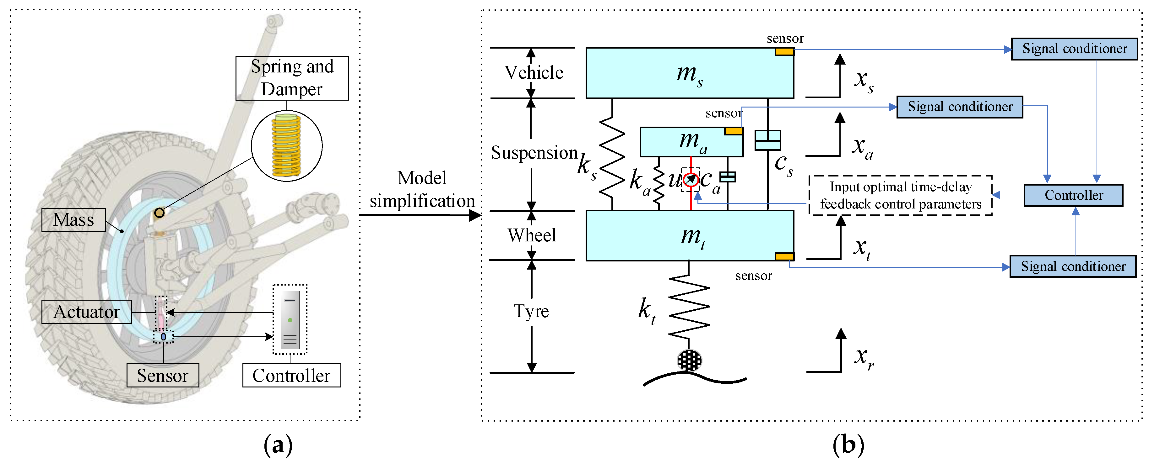
2. System Model of the New Wheel Structure
2.1. Mathematical Model
2.2. Preliminary Design of Parameters
2.3. Dimensionless System Model
3. Stability Analysis
3.1. Time-Delay Independent Stability
3.2. Time-Delay Dependent Stability
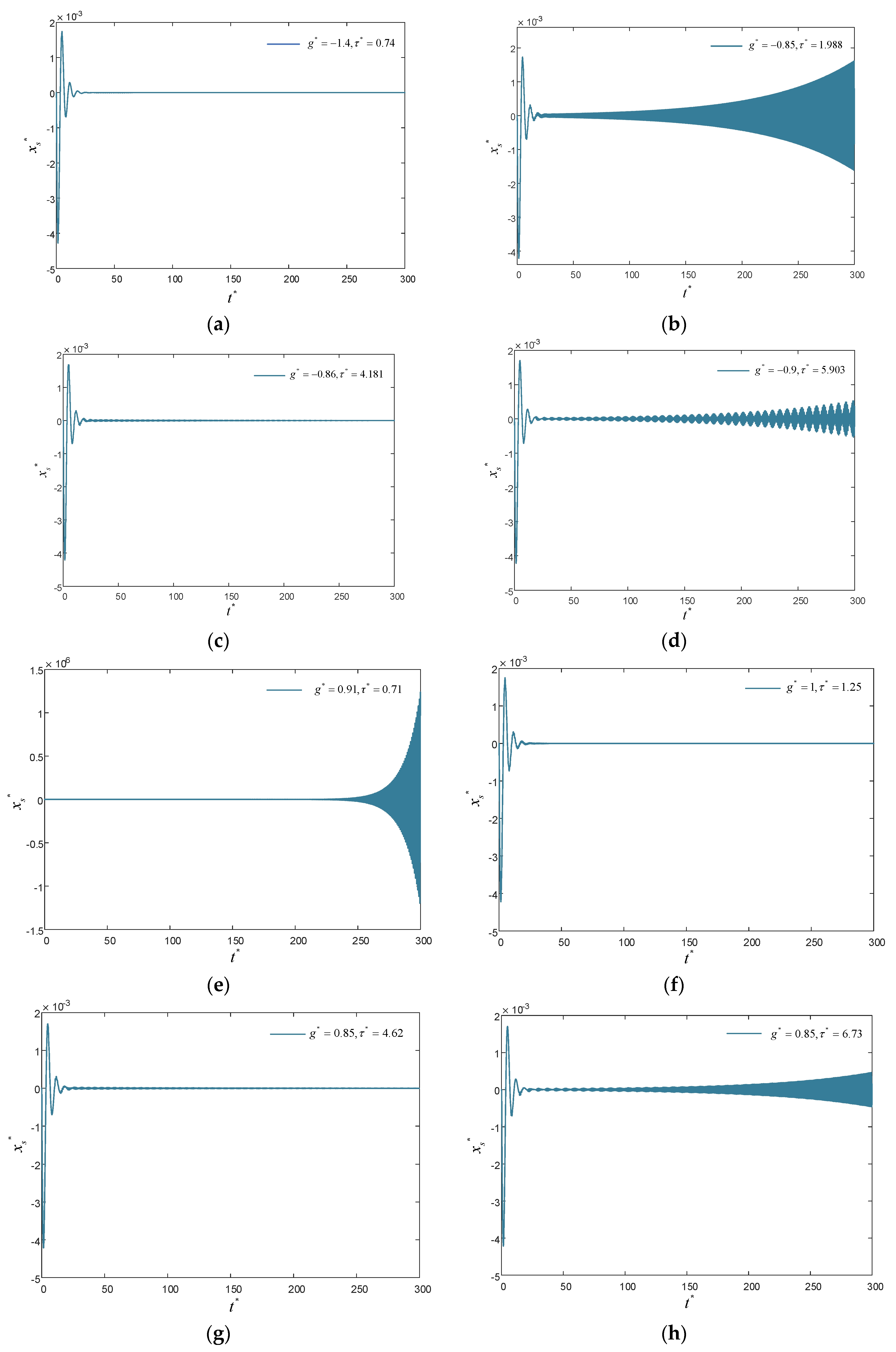
3.3. Numerical Simulation Verification
4. Objective Function and Optimization Design
4.1. Objective Function
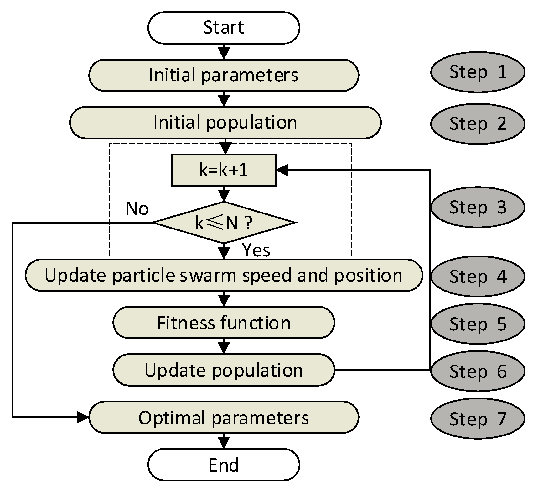
4.2. Optimization Procedure
- Step 1: Initialization parameters, including the time-delay , feedback gain , population size (pop_size = 50), number of iterations (N = 200), maximum velocity (), initial position(), initial velocity (), inertia weight (), and learning factors (). The position of the particles in each dimension is restricted to the selected area and the maximum velocity is a certain fraction of the search space range in each dimension.
- Step 2: Randomly generate the initial population, and temporarily record it as the population optimum, and then find the optimal particle in the population and record it as the global optimum.
- Step 3: Record the number of iterations of the system and compare the current number of iterations with the maximum number of iterations.
- Step 4: Based on the original population, the population position is updated by the PSO for the iteration, as shown in Equation (27).where is the current number of iterations; and are random parameters between ; is the individual optimal particle position; is the global optimal particle position; is the particle velocity; and is the current position of the particle. The start inertia weight is , end inertia weight is , and the current inertia weight is
- Step 5: In the optimization process, the objective function is also called the fitness function. The performance of the new structure is determined by the time delay () and the feedback gain coefficient (). The minimum value of the fitness function is obtained by optimizing these two parameters.
- Step 6: The particle positions updated in Step 4 are brought into the function in Step 5, and the new fitness function values are calculated. Each particle adaptation value is compared in an iterative search process, and the particle that produces a smaller value of fitness function is retained.
- Step 7: When the number of cycles reaches the set number of iterations , the system outputs the optimal parameters.
5. Results Analysis
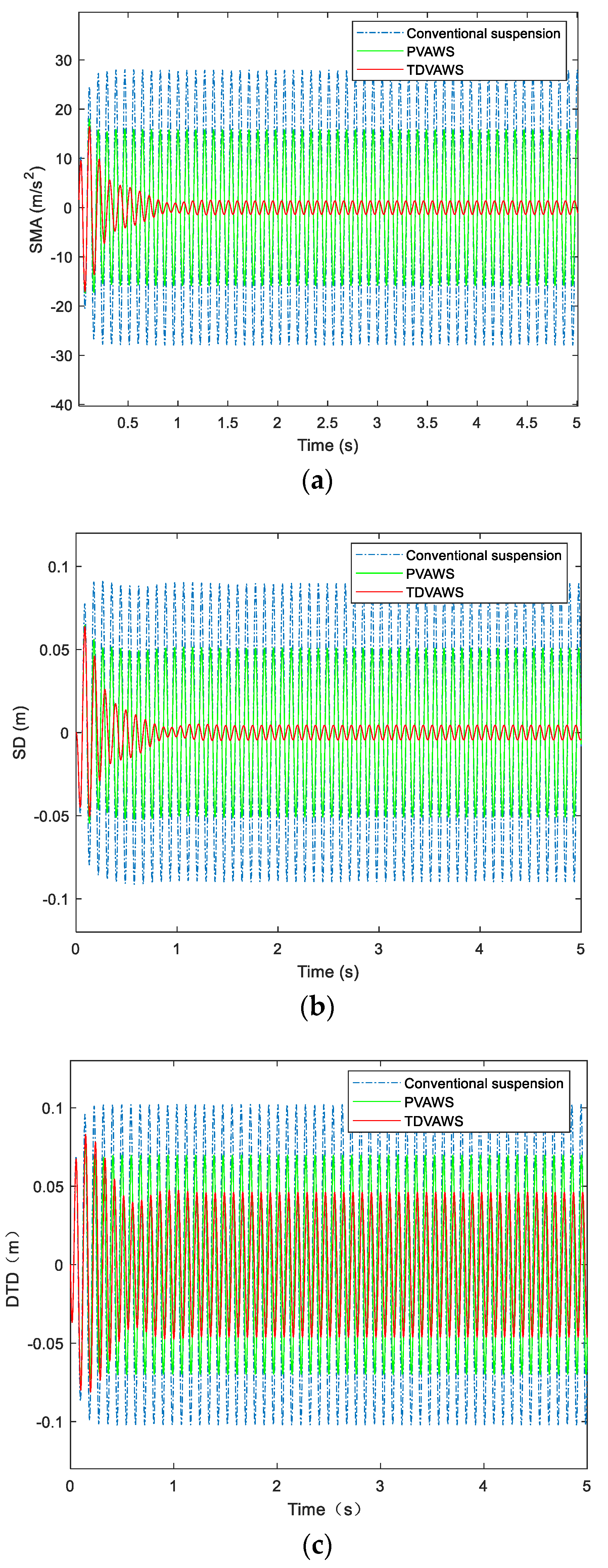
5.1. Simulation Analysis under Harmonic Excitation
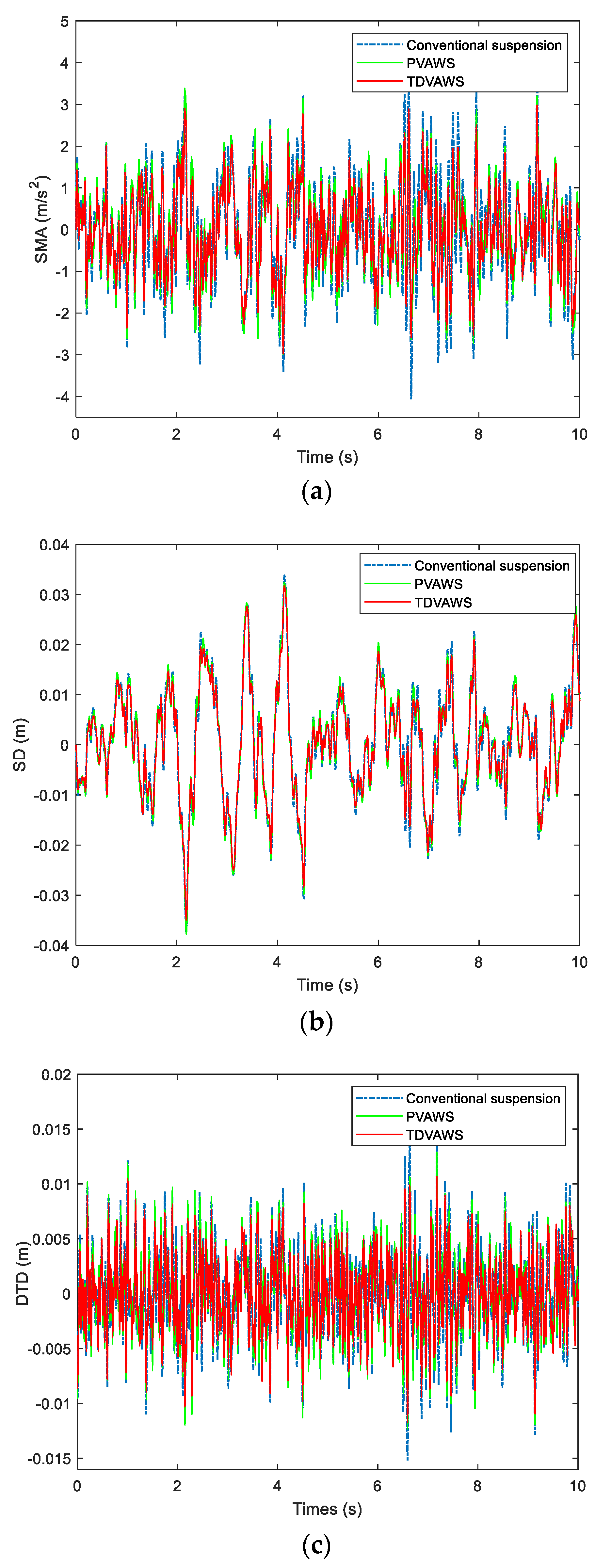
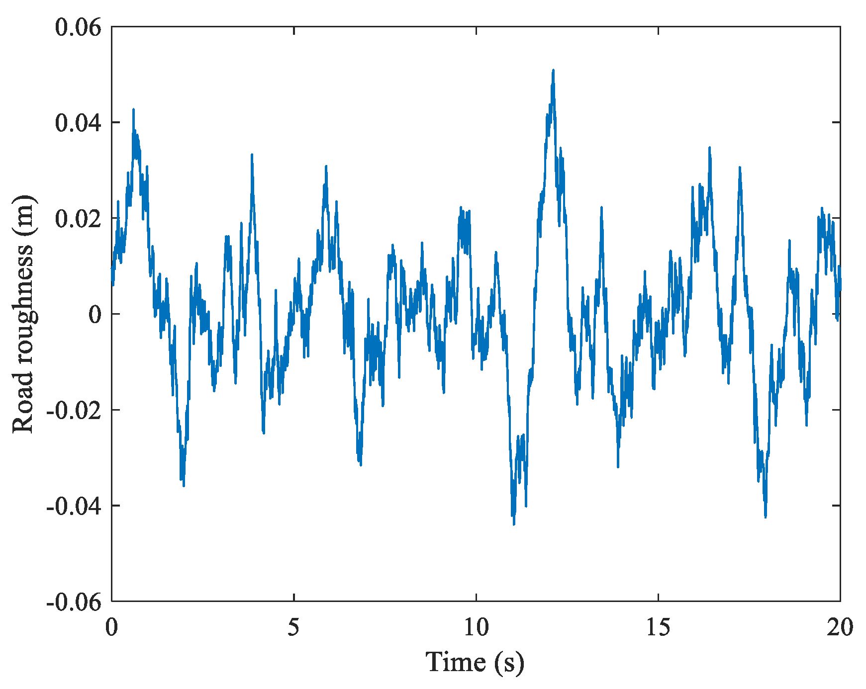
5.2. Simulation Analysis under Random Excitation
6. Conclusions
Author Contributions
Funding
Institutional Review Board Statement
Informed Consent Statement
Data Availability Statement
Conflicts of Interest
Appendix A
References
- Lu, J.B.; DePoyster, M. Multiobjective optimal suspension control to achieve integrated ride and handling performance. IEEE Trans. Control Syst. Technol. 2002, 10, 807–821. [Google Scholar]
- Luo, Y.; Wu, J.L.; Fu, W.K.; Zhang, Y.Q. Robust design for vehicle ride comfort and handling with multi-objective evolutionary algorithm. SAE Tech. Pap. 2013, 1, 415. [Google Scholar] [CrossRef]
- Els, P.S.; Theron, N.J.; Uys, P.E.; Thoresson, M.J. The ride comfort vs. handling compromise for off-road vehicles. J. Terramech. 2007, 44, 303–317. [Google Scholar] [CrossRef] [Green Version]
- Huang, S.J.; Lin, C.W. Application of a fuzzy enhance adaptive control on active suspension system. Int. J. Comput. Appl. Technol. 2004, 20, 152–160. [Google Scholar] [CrossRef]
- Sun, W.C.; Zhao, Z.L.; Gao, H.J. Saturated adaptive robust control for active suspension systems. IEEE Trans. Ind. Electron. 2013, 60, 3889–3896. [Google Scholar] [CrossRef]
- Xu, J.Q.; Chen, C.; Sun, Y.G.; Rong, L.J.; Lin, G.B. Nonlinear dynamic characteristic modeling and adaptive control of low speed maglev train. Int. J. Appl. Electromagn. Mech. 2019, 62, 73–92. [Google Scholar] [CrossRef]
- Sam, Y.M.; Osman, J.H.S.; Ghani, M.R.A. A class of proportional-integral sliding mode control with application to active suspension system. Syst. Control Lett. 2004, 51, 217–223. [Google Scholar] [CrossRef]
- Zhu, S.J.; He, Y.P.; Ren, J. Design of vehicle active suspension system using discrete-time sliding mode control with parallel genetic algorithm. In Proceedings of the ASME 2013 International Mechanical Congress and Exposition, San Diego, CA, USA, 15–21 November 2013. [Google Scholar]
- Du, H.P.; Sze, K.Y.; Lam, J. Semi-active H∞ control of vehicle suspension with magneto-rheological dampers. J. Sound Vib. 2005, 283, 981–996. [Google Scholar] [CrossRef]
- Gao, H.J.; Sun, W.C.; Shi, P. Robust sampled-data H∞ control for vehicle active suspension systems. IEEE Trans. Control Syst. Technol. 2010, 18, 238–245. [Google Scholar] [CrossRef]
- Zeng, M.Y.; Tan, B.H.; Ding, F.; Zhang, B.J.; Zhou, H.T.; Chen, Y.C. An experimental investigation of resonance sources and vibration transmission for a pure electric bus. Proc. Inst. Mech. Eng. Part D J. Automob. Eng. 2019, 234, 950–962. [Google Scholar] [CrossRef]
- Agrawal, A.K.; Fujino, Y.; Bhartia, B.K. Instability due to time delay and its compensation in active control of structures. Earthq. Eng. Struct. Dyn. 1993, 22, 211–224. [Google Scholar] [CrossRef]
- Chen, L.; Wang, R.C.; Jiang, H.B.; Zhou, L.K.; Wang, S.H. Time delay on semi-active suspension and control system. Chin. J. Mech. Eng. 2006, 42, 130–133. [Google Scholar] [CrossRef]
- Han, S.Y.; Tang, G.Y.; Chen, Y.H.; Yang, X.X.; Yang, X. Optimal vibration control for vehicle active suspension discrete-time systems with actuator time delay. Asian J. Control 2013, 15, 1579–1588. [Google Scholar] [CrossRef]
- Chen, S.A.; Zu, G.H.; Yao, M.; Zhang, X.N. Taylor series-LQG control for time delay compensation of magneto-rheological semi-active suspension. J. Vib. Shock 2016, 36, 190–243. [Google Scholar]
- Olgac, N.; Holm-Hansen, B.T. A novel active vibration absorption technique: Delayed resonator. J. Sound Vib. 1994, 176, 93–104. [Google Scholar] [CrossRef]
- Olgac, N.; Holm-Hansen, B. Design considerations for delayed-resonator vibration absorbers. J. Eng. Mech. 1995, 121, 80–89. [Google Scholar] [CrossRef]
- Fridman, E. New Lyapunov–Krasovskii functionals for stability of linear retarded and neutral type systems. Syst. Control Lett. 2001, 43, 309–319. [Google Scholar] [CrossRef]
- Gu, K. An improved stability criterion for systems with distributed delays. Int. J. Robust Nonlinear Control 2003, 13, 819–831. [Google Scholar] [CrossRef]
- Wang, Z.H.; Hu, H.Y. Stability switches of time-delayed dynamic systems with unknown parameters. J. Sound Vib. 2000, 233, 215–233. [Google Scholar] [CrossRef]
- Li, X.G. Some Studies on the Stability of Time-Delay Systems. Ph.D. Thesis, Shanghai Jiao Tong University, Shanghai, China, 2007. [Google Scholar]
- Zeng, H.B.; He, Y.; Wu, M.; She, J. Free-matrix-based integral inequality for stability analysis of systems with time-varying delay. IEEE Trans. Autom. Control 2015, 60, 2768–2772. [Google Scholar] [CrossRef]
- Lee, J.; Medrano-cerda, G.A.; Jung, J.H. Stability analysis for time delay control of nonlinear systems in discrete-time domain with a standard discretisation method. Control Theor. Tech. 2020, 18, 92–106. [Google Scholar] [CrossRef]
- Huang, L.; Chen, C.; Huang, S.J.; Wang, J.F. Stability of real-time hybrid simulation involving time-varying delay and direct integration algorithms. J. Vib. Control 2021. [Google Scholar] [CrossRef]
- Zhang, J.; Zhang, B.J.; Zhang, N.; Chen, Y.C. A novel reliable robust adaptive event-triggered automatic steering control approach of autonomous land vehicles under communication delay. Int. J. Robust Nonlinear Control 2021, 31, 2436–2464. [Google Scholar] [CrossRef]
- Jalili, N.; Olgac, N. A sensitivity study on optimum delayed feedback vibration absorber. J. Dyn. Syst. Meas. Control 2020, 122, 314–321. [Google Scholar] [CrossRef]
- Jalili, N.; Olgac, N. Identification and retuning of optimum delayed feedback vibration absorber. J. Guid. Control Dyn. 2020, 23, 961–970. [Google Scholar] [CrossRef]
- Udwadia, F.E.; Phohomsiri, P. Active control of structures using time delayed positive feedback proportional control designs. Struct. Control Health Monit. 2006, 13, 536–552. [Google Scholar] [CrossRef]
- Zhao, Y.Y.; Xu, J. Mechanism analysis of delayed nonlinear vibration absorber. Chin. J. Theor. Appl. Mech. 2008, 40, 98–106. [Google Scholar]
- Yan, T.H.; Ren, C.B.; Zhou, J.L.; Shao, S.J. The study on vibration reduction of nonlinear time-delay dynamic absorber under external excitation. Math. Prob. Eng. 2020, 14, 8578596. [Google Scholar] [CrossRef] [Green Version]
- Huan, R.H.; Chen, L.X.; Sun, J.Q. Multi-objective optimal design of active vibration absorber with delayed feedback. J. Sound Vib. 2014, 339, 56–64. [Google Scholar] [CrossRef]
- Wu, K.W.; Ren, C.B.; Cao, J.S.; Sun, Z.C. Reach on damping control and stability analysis of vehicle with double time-delay and five degrees of freedom. J. Low Freq. Noise, Vib. Act. Control 2020, 40, 1024–1039. [Google Scholar] [CrossRef]
- Wu, K.W.; Ren, C.B. Control and stability analysis of double time-delay active suspension based on particle swarm optimization. Shock Vib. 2020, 8, 8873701. [Google Scholar] [CrossRef]
- Asami, T.; Nishihara, O.; Baz, A.M. Analytical solutions to H∞ and H2 optimization of dynamic vibration absorbers attached to damped linear systems. J. Vib. Acoust. 2002, 124, 284–295. [Google Scholar] [CrossRef]
- Fang, J.; Wang, S.M.; Wang, Q. Optimal design of vibration absorber using minimax criterion with simplified constraints. Acta Mech. Sin. 2012, 28, 848–853. [Google Scholar] [CrossRef]
- Shao, S.J.; Ren, C.B.; Jing, D.; Yan, T.H. Stability, bifurcation and chaos of nonlinear active suspension system with time delay feedback control. J. Vib. Shock 2021, 40, 281–290. [Google Scholar]
- Hu, W.; Li, Z.S. A simpler and more effective particle swarm optimization algorithm. J. Softw. 2007, 18, 861–868. [Google Scholar]
- Chen, J.P.; Chen, W.W.; Zhu, H.; Zhu, M.F. Modeling and simulation on stochastic road surface irregularity based on MATLAB/Simulink. Trans. Chin. Soc. Agric. Mach. 2010, 41, 11–15. [Google Scholar]
- Ma, K.H.; Ren, C.B.; Zhang, Y.G.; Xu, Z. The influence of different displacement time-delay feedback control on vehicle body vibration reduction. Sci. Technol. Eng. 2021, 21, 12259–12267. [Google Scholar]
 Time-delay independent stability region;
  Time-delay dependent stability region;
  Unstable region.
Time-delay independent stability region; Time-delay dependent stability region; Unstable region.
Unstable region.
Time-delay independent stability region; Time-delay dependent stability region; Unstable region.
 Stable region;
  Unstable region.


| Parameters | Value | Parameters | Value |
|---|---|---|---|
| (kg) | 345 | cs (N·s/m) | 1500 |
| (kg) | 40.5 | g (N·s/m) | −30,000~30,000 |
| (N/m) | 17,000 | τ (s) | 0~1 |
| (N/m) | 192,000 |
| 0.1 | 4.05 | 18,136.36 | 82.62 |
| 0.2 | 8.10 | 31,930.56 | 212.28 |
| 0.3 | 12.15 | 42,665.68 | 356.97 |
| 0.4 | 16.20 | 51,183.67 | 506.61 |
| Parameters | Value | Parameters | Value |
|---|---|---|---|
| 0.6194 | −1.7647~1.7647 | ||
| 0~0.0909 | 11.2941 | ||
| 42.5926 | 1.8783 | ||
| 8.5185 | 0~7.0196 |
| Region | |||
|---|---|---|---|
| s1 | + − − − − − + + + − + | 1, 1, −1, 1, 1, 1, 1, −1, 1, 1, −1, 1 | 0 |
| s2 | + + − − − − + + + − + | 1, 1, 1, −1, 1, 1, 1, −1, 1, 1, −1, 1 | 0 |
| s3 | + + − − − − − + + − + | 1, 1, 1, −1, 1, 1, 1, 1, −1, 1, −1, 1 | 0 |
| s4, s5 | + + − − − − − − − + + | 1, 1, 1, −1, 1, 1, 1, 1, 1, 1, −1, 1 | 4 |
| s6, s7 | + + − + − − − − − + + | 1, 1, 1, −1, −1, −1, 1, 1, 1, 1, −1, 1 | 4 |
| s8, s9 | + + + + − − − − − + + | 1, 1, 1, 1, 1, −1, 1, 1, 1, 1, −1, 1 | 4 |
| s10, s11 | + + + + + − − − − + + | 1, 1, 1, 1, 1, 1, −1, 1, 1, 1, −1, 1 | 4 |
| s12, s13 | + + + − + − − − − + + | 1, 1, 1, 1, −1, −1, −1, 1, 1, 1, −1, 1 | 4 |
| s14, s15 | + + + − − − − − − + + | 1, 1, 1, 1, −1, 1, 1, 1, 1, 1, −1, 1 | 4 |
| Performance Indexes | Conventional Suspension | PVAWS | TDVAWS |
|---|---|---|---|
| 19.7211 | 11.1859 | 1.4964 | |
| 63.3691 | 35.9532 | 5.1521 | |
| 72.0473 | 49.3270 | 33.0481 |
| Performance Indexes | Conventional Suspension | PVAWS | TDVAWS |
|---|---|---|---|
| 1.2342 | 1.1158 | 1.0465 | |
| 11.0682 | 11.0286 | 11.0089 | |
| 4.0993 | 3.9222 | 3.5861 |
Publisher’s Note: MDPI stays neutral with regard to jurisdictional claims in published maps and institutional affiliations. |
© 2022 by the authors. Licensee MDPI, Basel, Switzerland. This article is an open access article distributed under the terms and conditions of the Creative Commons Attribution (CC BY) license (https://creativecommons.org/licenses/by/4.0/).
Share and Cite
Ma, K.; Ren, C.; Zhang, Y.; Chen, Y.; Chen, Y.; Zhou, P. A New Vibration-Absorbing Wheel Structure with Time-Delay Feedback Control for Reducing Vehicle Vibration. Appl. Sci. 2022, 12, 3157. https://doi.org/10.3390/app12063157
Ma K, Ren C, Zhang Y, Chen Y, Chen Y, Zhou P. A New Vibration-Absorbing Wheel Structure with Time-Delay Feedback Control for Reducing Vehicle Vibration. Applied Sciences. 2022; 12(6):3157. https://doi.org/10.3390/app12063157
Chicago/Turabian StyleMa, Kehui, Chuanbo Ren, Yongguo Zhang, Yuanchang Chen, Yajie Chen, and Pengcheng Zhou. 2022. "A New Vibration-Absorbing Wheel Structure with Time-Delay Feedback Control for Reducing Vehicle Vibration" Applied Sciences 12, no. 6: 3157. https://doi.org/10.3390/app12063157
APA StyleMa, K., Ren, C., Zhang, Y., Chen, Y., Chen, Y., & Zhou, P. (2022). A New Vibration-Absorbing Wheel Structure with Time-Delay Feedback Control for Reducing Vehicle Vibration. Applied Sciences, 12(6), 3157. https://doi.org/10.3390/app12063157