Development of Automatic Crack Growth Simulation Program Based on Finite Element Analysis

Featured Application

Crack Growth Assessment for Fracture Mechanics.

Abstract

A crack growth simulation program based on the advanced iterative-finite element method (AI-FEM) was developed to predict realistic crack growth of structures. The developed program was suggested to calculate the exact stress intensity factor for arbitrary structures by regenerating the crack tip mesh as the crack grows. The main advantages of the developed program are to estimate each different crack growths along the crack tip line and to simulate the cracking transition from a surface crack to a through-wall crack under a complex stress field. For these purposes, the sensitivity analyses were performed for various influence variables on stress intensity factors, such as element types and crack dimensions. Based on the results of sensitivity analyses, the appropriate criteria for crack tip modeling to be used in AI-FEM were suggested to calculate sufficient converged SIF. The program developed in this research was validated through stress corrosion crack growth and natural crack growth examples including cracking transition, and it was confirmed that the program simulates crack growth well and has reasonable methods for cracking transition.

1. Introduction

Alloy 600 and 82/182 have been widely used as base and welding materials in various components of nuclear power plants (NPP) [1]. However, these materials are susceptible to primary water stress corrosion cracking (PWSCC), and cracking due to PWSCC has been reported in many NPPs as operation time increases [2,3]. If cracks are detected during operation, a comparison of acceptance standards and crack size should be performed according to ASME code, Sec. XI [4]. If the crack does not exceed the allowable crack size in the ASME code, it can continue to operate without maintenance, whereas if the crack exceeds the allowable limit, a fracture mechanics evaluation should be performed. To evaluate the cracked structure based on ASME code, the natural crack with arbitrary shape is idealized as an elliptical surface crack for conservative and efficient evaluation. The final crack size can be determined through fatigue crack growth (FCG) evaluation by calculating stress intensity factor (SIF), which is a representative linear elastic fracture mechanics parameter. In addition, the shape of crack growth is assumed to maintain an elliptical shape, so that crack growths are estimated only at the surface and deepest points. However, such an evaluation method can overly conservatively evaluate the integrity of a structure as in the case of the Wolf Creek NPP, which may result in unnecessary maintenance costs [5].

This conservatism can be improved by directly evaluating the crack growth at the crack tip of a natural crack rather than evaluating the idealized crack growth. To evaluate the growth of real cracks with complex geometries, various studies have been conducted based on finite element analysis (FEA). The finite-discrete element method [6,7,8] has been employed for impact failure of monolithic glass, layered composite material, and functionally graded materials.

Furthermore, the phase-field and extended finite element method based on damage fracture mechanics [9,10,11,12] have been known to be powerful to simulate brittle cracking and anisotropic fracture. However, high nonlinearity in the numerical analysis process is unavoidable using these methods, so the applicability of these methods to various components in NPP is not fully investigated yet.

For this reason, conventional FEA based on the linear elastic fracture mechanics using the spider-web mesh at the crack tip has been generally considered as the reliable approach of crack growth assessment for structures in NPP. However, high proficiency in modeling techniques is required to generate the spider-web mesh at the crack tip. To overcome these difficulties, crack growth evaluation programs were also developed based on relative research. Hou et al. [13] developed ZENCRACK, a program that can simulate 3D crack growth based on Abaqus. However, this program cannot simulate the transition from a surface crack to a through-wall crack and it is difficult to accurately simulate the crack growth due to the combined load because the combined load is applied replacing it with an equivalent load. In Emc², AFEA (Advanced Finite Element Analysis), a method that can simulate crack growth through crack tip mesh regeneration without assuming a semi-elliptical crack, was developed [14]. Using this program, crack growth analysis was performed for nozzles in the PWSCC environment, and the safety margin of the structure was verified by comparing typical ASME code, Sec. XI-type analysis. As a follow-up study, Shim et al. [15] simulated cracking transition as a through-wall crack by performing crack growth of a pipe with semi-elliptical inner surface cracks in a primary water environment. Nakamura et al. [16] developed FINAS/CRACK, automatic crack growth and fatigue evaluation program, and based on the standard low-cycle fatigue theory, calculate the amount of FCG at each point along the crack front to simulate natural crack growth. The results of crack growth using the program were verified by comparison with the test results performed by Nakamura et al. [17]. Ogawa et al. [18] performed stress corrosion crack (SCC) growth by automatic re-meshing for natural cracks of dissimilar metals using Abaqus and in-house code. This was verified by comparison with the crack growth test in a water environment. As such, various re-meshing techniques have been developed for crack growth modeling based on FEA. However, existing studies have focused on one of the FCG and SCC growth. In addition, these methods and programs have limited application to various geometries such as nozzles.

This study developed the advanced iterative-finite element method (AI-FEM), a python-based automatic crack growth program that operates as a plug-in program in Abaqus. AI-FEM is based on linear elastic fracture mechanics, and the SIF is calculated along the crack front. For arbitrary crack shape, mechanical FCG and SCC growth behavior can be simulated as a non-idealized crack shape by utilizing the developed program. Sensitivity analyses were performed on various variables affecting the SIF value and crack tip element shape such as the number of elements in the circumferential direction inside the contour and radial direction of the contour. The appropriate criteria for crack tip modeling that can be applied as default settings of the program or can be referenced when using the program are presented. The developed program was verified by comparing it with the SCC growth calculated by the procedure presented in ASME code, Sec. XI. In addition, SCC growth verification was additionally performed in comparison with natural crack growth, and the validity of the specified cracking transition method was verified.

2. Development of AI-FEM

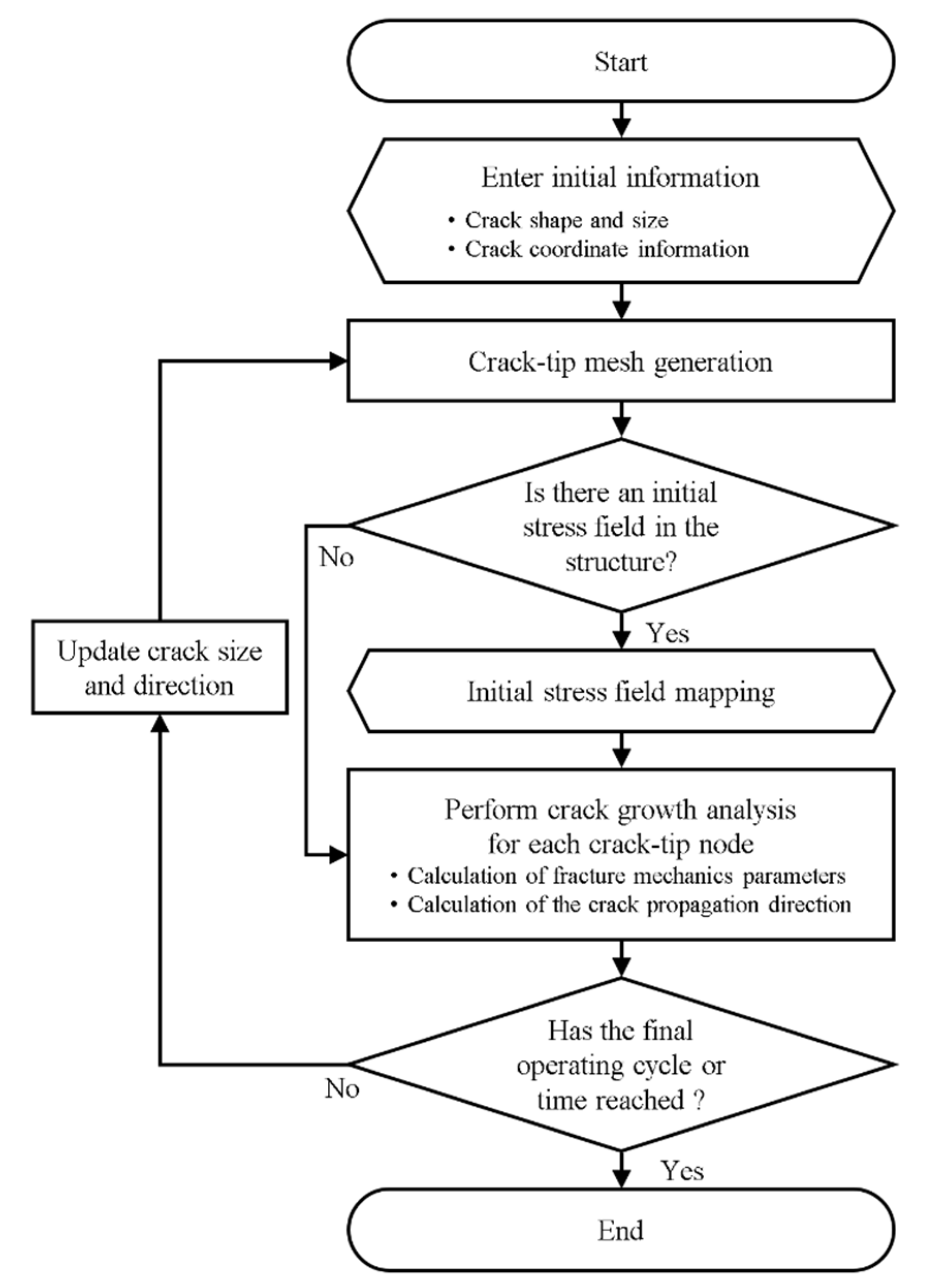
2.1. The Overall Procedures of AI-FEM

The crack growth evaluation procedure through AI-FEM is shown in Figure 1. As a first step, information of initial crack is entered such as initial crack shape and location. Then, the program generates a crack tip mesh based on the initial crack information and the modeling criteria described in Section 2.2. If there is an initial stress field such as the weld residual stress considered in the MRP-215 report [19], stress mapping is performed using the ‘Map Solution’ function provided by Abaqus [20]. If the initial stress field does not exist, this step can be omitted. Once the crack information, load, and stress conditions are all entered, AI-FEM calculates the SIF (K_I) values at each node along the crack tip and crack growth direction. By applying SIF to the FCG curve or the SCC growth curve, the corresponding crack growth length can be calculated, and the crack growth direction can be determined as the normal direction at each point along the crack tip. In the next step, the AI-FEM checks whether the final operating cycle for FCG or time for SCC has been reached. If the final operating cycle or time is not reached, the crack size is updated by adding the crack growth length to the current crack size at each point along the crack tip. Using the updated crack information, the crack tip mesh is regenerated, and the above-mentioned process is repeated until the final operation cycle or time is reached.

2.2. Crack Tip Meshing Criteria

In order to calculate SIF by FEA efficiently, it is necessary to be able to calculate accurate SIF with minimum mesh density. In particular, to calculate SIF accurately, the effect of variables on SIF (calculation method, element type, crack tip singularity, element shape variables) should be examined. In this section, the guidelines of crack tip modeling were presented by analyzing various variables affecting SIF using a flat plate with a semi-elliptical surface crack under tensile load.

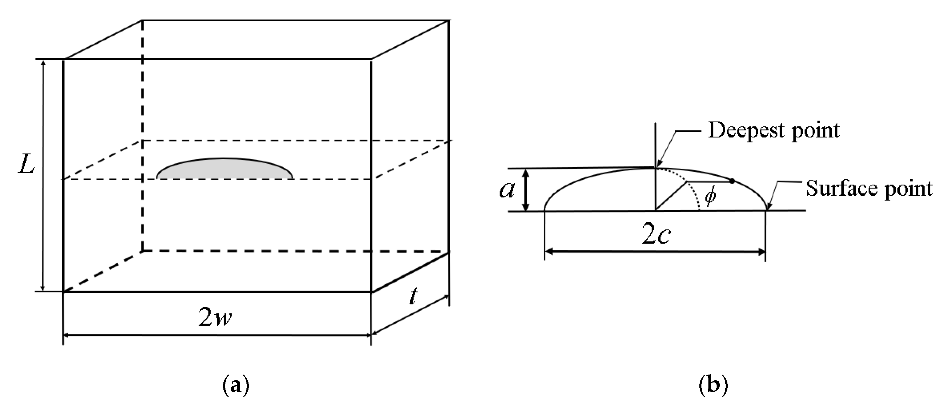
2.2.1. Geometry and Materials

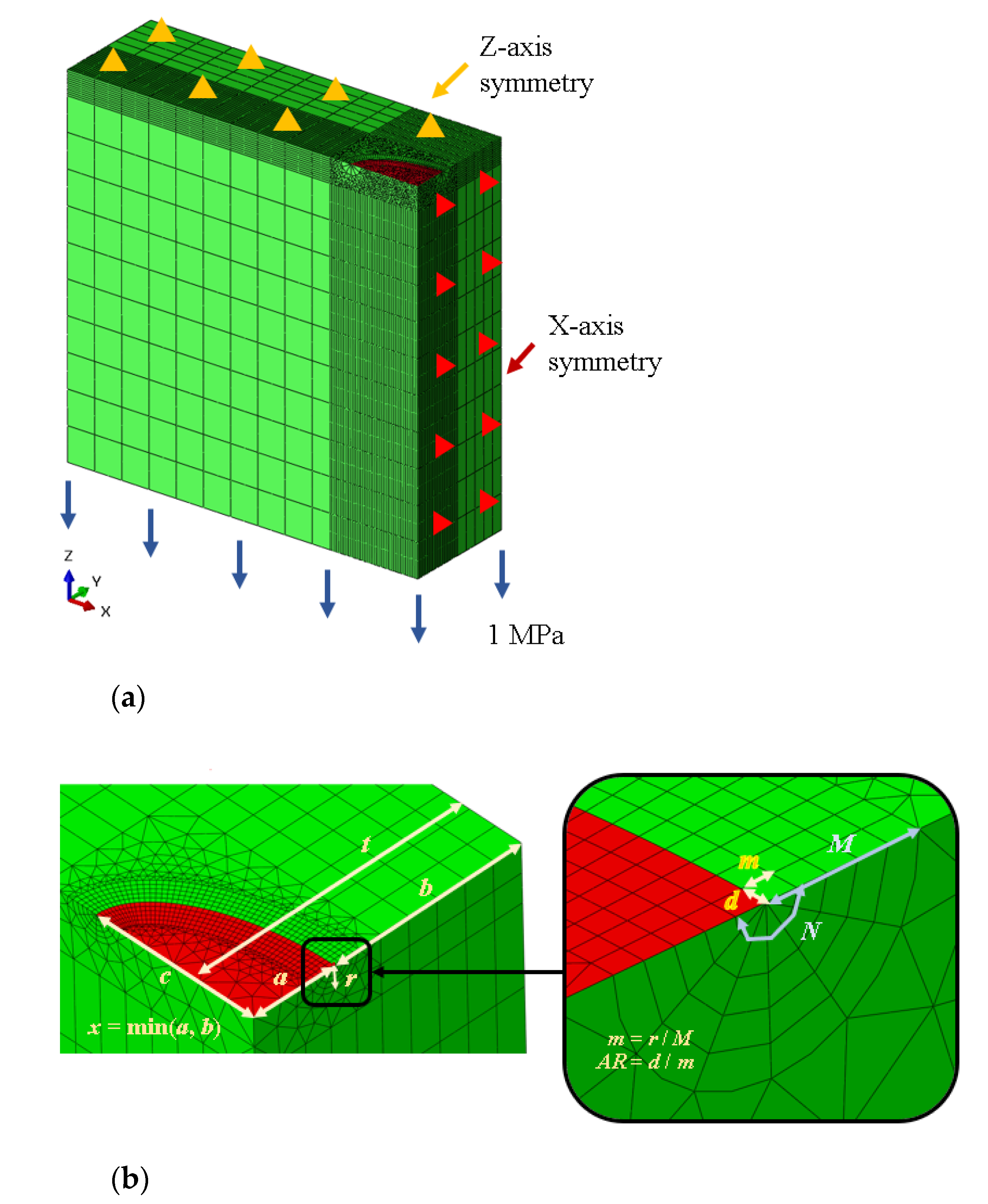
Figure 2 is a schematic of a flat plate with a semi-elliptical surface crack. Figure 2a shows the overall shape of the cracked plate, and Figure 2b shows the shape variables of semi-elliptical surface crack. In Figure 2a, L, w, and t mean the vertical length, half of the horizontal length, and thickness of the plate, respectively. In Figure 2b, a, c and ø represent the crack depth, half of the crack length, and crack angle, respectively. As shown in

Table 1. Shape variables of plates with semi-elliptical surface crack.

w/t	a/t	a/c
3.15	0.3	0.5

, w/t = 3.15, a/t = 0.3, and a/c = 0.5 were considered as the shape variables of the plate in the SIF sensitivity analyses. The elastic modulus (E) was considered to be 200 GPa, and the Poisson’s ratio (v) was considered to be 0.3.

2.2.2. FE Model

Figure 3a shows the FE model and boundary conditions of a plate with a crack. Considering the symmetry of geometry, a 1/4 symmetric model was used, and symmetry conditions were applied to each symmetrical plane. As a loading condition, a tensile distribution load of 1 MPa in the Z-axis direction was considered. Except for the case of performing sensitivity analysis on element types, the element type was considered as a 20-node brick element with reduced integration (C3D20R in Abaqus library). The middle node of the wedge element was located at the center position, and the overlapping state of the crack tip nodes was considered as a basic element characteristic condition.

Figure 3b shows the detailed shape of the crack tip mesh and the shape variables constituting the crack tip mesh. x means the shorter of the crack depth (a) and the residual length (b), and r means the contour radius of the spider-wedge mesh. r and x are used as dimensionless variables as r/x and the effect of the contour radius on the SIF is considered. Also, since r/x is the ratio of the relative contour size to the crack size, the size of the contour mesh can be defined in the plate if r/x is in between zero and one. N and M are the numbers of elements in the circumferential direction inside the contour and radial direction of the contour, respectively. m is defined as r/M and represents the element size in the radial direction inside the contour. AR is defined as d/m and represents the ratio of the total length of the crack tip to the radial size of the element. As AR increases, the element density in the direction of the crack angle decreases relatively, and it is used as a non-dimensional variable to examine the sensitivity analyses of the SIF.

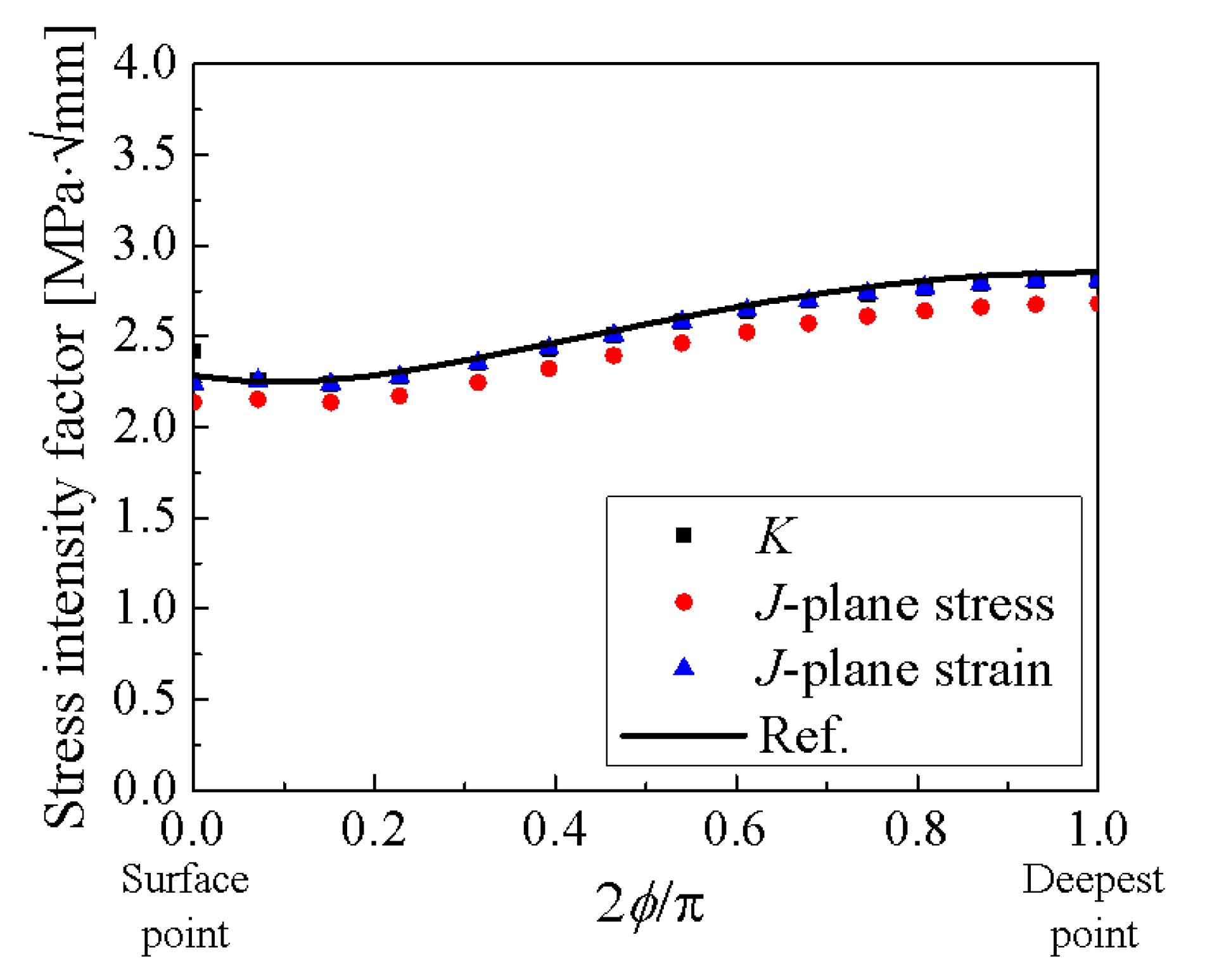
2.2.3. The Effect of the SIF Calculation Method

In this section, the SIF was calculated using the domain integral method and interaction integral method [21] provided by Abaqus. The elastic J-integral (J_e) can be obtained through the domain integral method, and the SIF for each plane stress and strain condition can be calculated through relations based on the fracture mechanics theory, respectively. The relation is as follows in Equation (1):

$$\begin{gathered} K_{FE}=\sqrt{J_e{E}^{\prime }} \\ {E}^{\prime }=E \mathrm{for}\mathrm{plane}\mathrm{stress} \\ {E}^{\prime }=\frac{E}{\left(1-v^2\right)} \mathrm{for}\mathrm{plane}\mathrm{strain} \end{gathered}$$

(1)

where K_FE is the SIF calculated through FEA.

The interaction integral method is a function that can directly calculate the SIF for each failure mode (mode I, II, III). To see the effect of the SIF calculation method the SIF for mode I was calculated. In both methods, the number of elements in the contour region should be determined in the FE model, and 5 contour elements are considered. The SIF was defined as the average value of contours 2 to 4 excluding the results from the first and last contours.

Figure 4 shows the difference in SIF according to the SIF calculation methods along the crack tip. In the domain integral method, the SIF values converted through the assumption of plane stress and plane strain were expressed as J-plane stress and J-plane strain, respectively, and the SIF value calculated through the interaction integration method was expressed as K. The SIF results were compared with the theoretical solution proposed by Raju-Newman [22] and the results of the theoretical solution are denoted as Ref. In Figure 4, J-plane strain and K show SIF values similar to those of Raju-Newman solution and J-plane stress slightly smaller. However, the plane stress and plane strain conditions can be changed depending on the shape and constraint of the structure. Therefore, in this study, the interaction integral method reflecting the constraint effect was selected as the SIF calculation method.

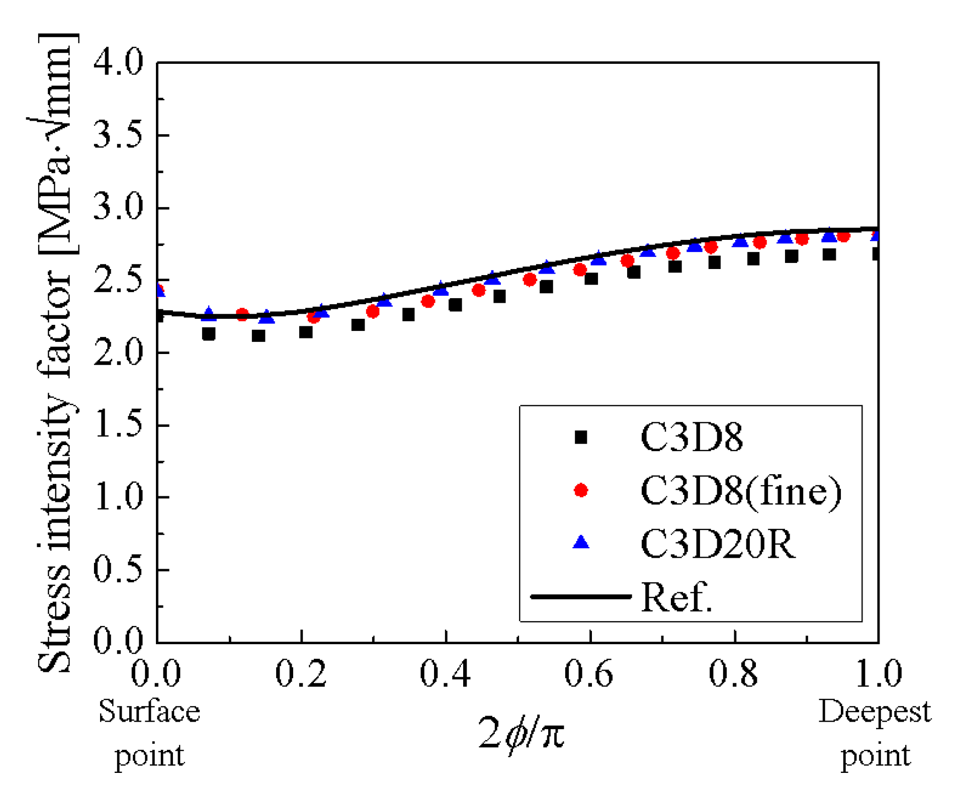
2.2.4. The Effect of Element Type

To consider the effect of element type on SIF, C3D8 (8-node brick element) and C3D20R (20-node brick element with reduced integration) were considered. For C3D8, the C3D8 (fine) model, which doubled the number of elements, was also considered to check the difference according to the number of elements. Figure 5 shows the difference in SIF according to the element type. The SIF using the C3D20R element was in good agreement with the Raju-Newman solution. In the case of the C3D8 element model, the result varies depending on the element density. Therefore, it is judged that it is reasonable to use C3D20R when generating a FE model for SIF calculation. In the subsequent section, C3D20R was applied to all sensitivity analyses.

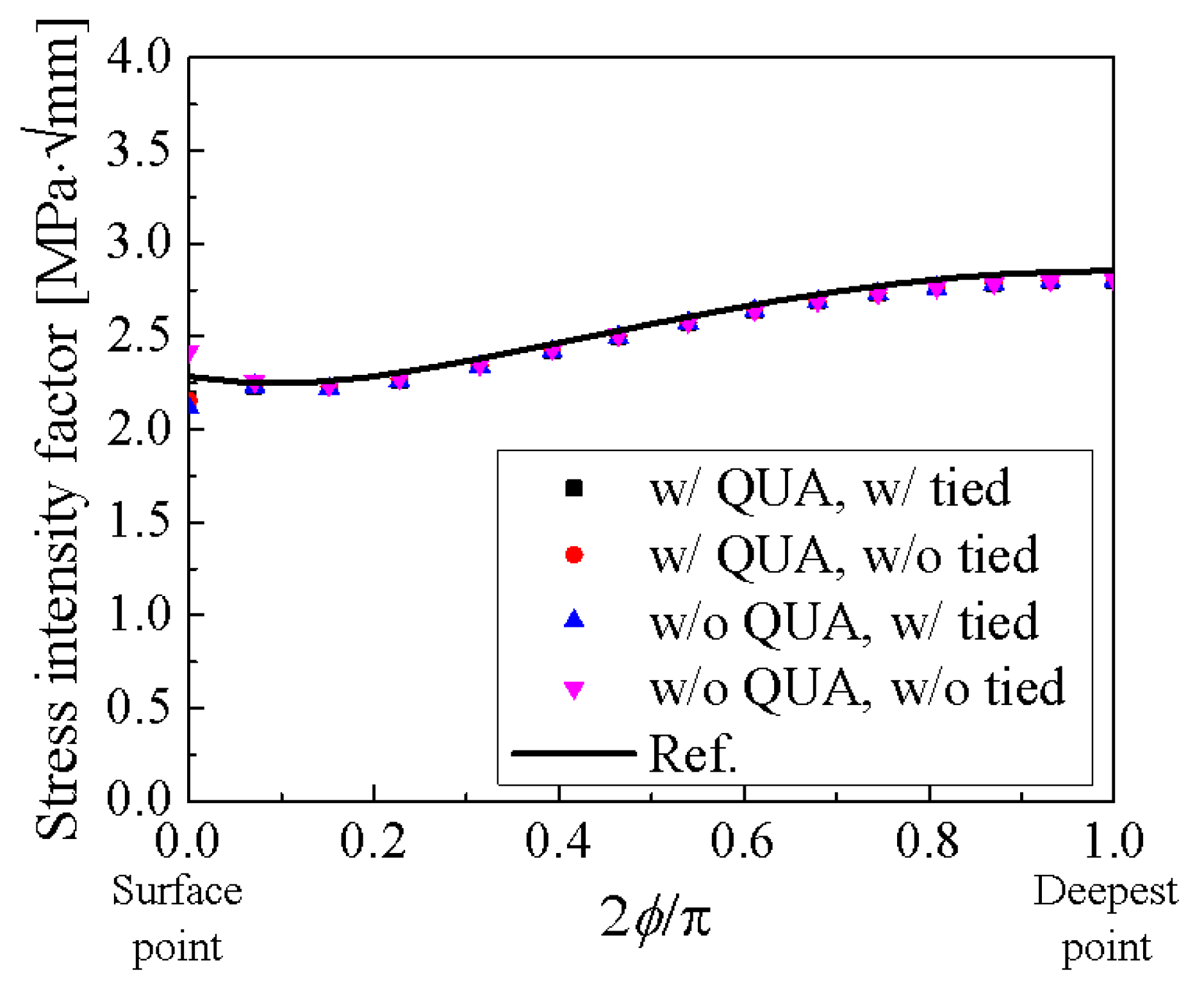
2.2.5. The Effect of Crack Tip Element Characteristic

In Abaqus, when generating a crack tip mesh, it should be determined whether to use a quarter-point element (QUA) and whether to use a crack tip overlapping (tied) node. In general, it is known that strain singularity appears, and numerical accuracy is improved when QUA and tied are used in elastic FEA [21]. However, since the contour integral option, which is the SIF calculation module of Abaqus, calculates the SIF using the domain integral method, it is known that the larger the contour area is set, the less the influence of the crack tip node location and overlap is known. Figure 6 shows the difference in the SIF according to the fracture mechanics setting of the wedge element when the secondary element is used for the mesh of the crack tip. w and w/o mean ‘with’ and ‘without’. The difference in the SIF at each setting was small, within about 0.5%. The difference in SIF calculated in the four cases depending on whether the two options were applied was small, within about 0.5%. Therefore, it was determined not to use these options in the modeling of crack tip mesh because the numerical accuracy improvement by applying these two options was insignificant.

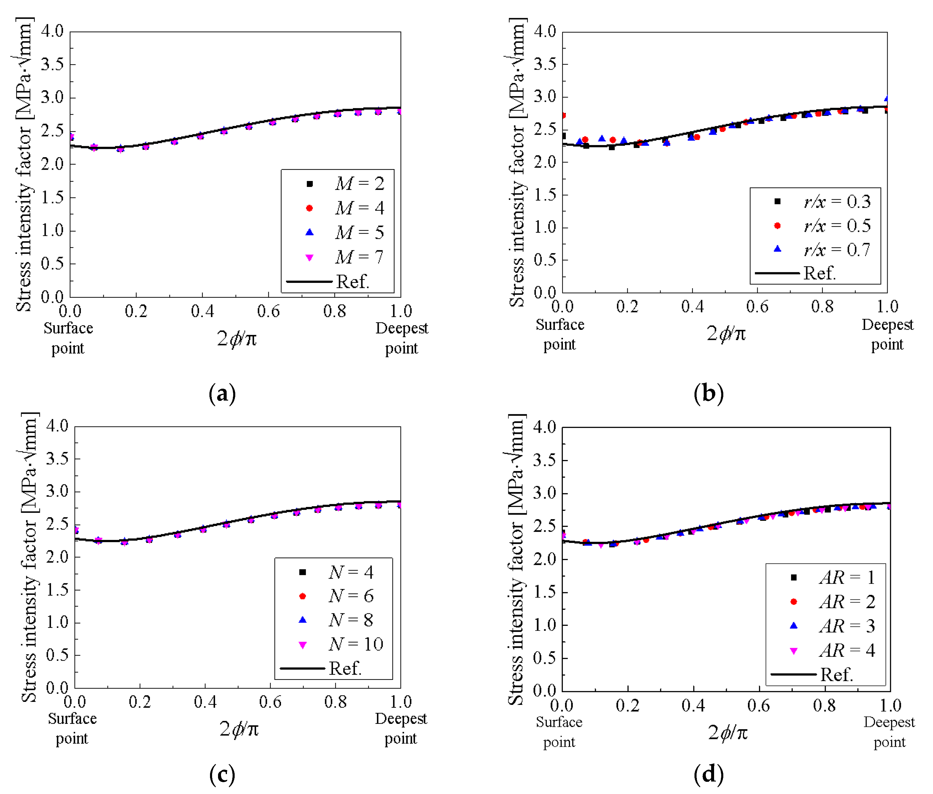
2.2.6. The Effect of Shape Variables of Crack Tip Mesh

When calculating SIF by FEA, a crack tip mesh is generally used, and the SIF value may vary depending on the element density of the crack tip mesh. In this section, sensitivity analysis was performed for various shape variables constituting the crack tip mesh such as M, r/x, N, and AR shown in Figure 3b. The range of shape variables considered for sensitivity analysis can be seen in

Table 2. Shape variables considered in the SIF sensitivity analyses.

M	r/x	N	AR
2, 4, 5, 7	0.3, 0.5, 0.7	4, 6, 8, 10	1, 2, 3, 4

. When the sensitivity analysis for one variable is performed, the other variables were fixed as shown in

Table 3. Fixed shape variables for SIF sensitivity analyses.

M	r/x	N	AR
5	0.3	6	1

. To check the effect of M, r/x, and N, crack of a/t = 0.3, a/c = 0.5 were assumed.

Figure 7 shows the difference in SIF according to shape variables. In all shape variables, the SIF shows a similar tendency to the Raju-Newman solution. However, at the surface point, it was different depending on the variables. To determine the shape variables applied to the program, firstly, it was checked whether the SIF converges at the surface point, and an intermediate value was set to avoid unexpected numerical errors among the converged variables. The determined shape variables are shown in

Table 4. Crack tip modeling guidelines suggested through SIF sensitivity analysis.

M	r/x	N	AR
5	0.3	8	1

.

3. Detailed Function of AI-FEM

3.1. Overview of the Program

AI-FEM is developed based on python and works as a plug-in program of Abaqus, a commercial FEA program. The overall graphical user interface (GUI) of AI-FEM is shown in Figure 8. The program can be applied to any structure geometry into which crack cells can be inserted, including 2D/3D plates and pipe models. In addition, the program can select 4 smoothing methods to avoid creating inaccurate meshes that can occur when updating crack growth.

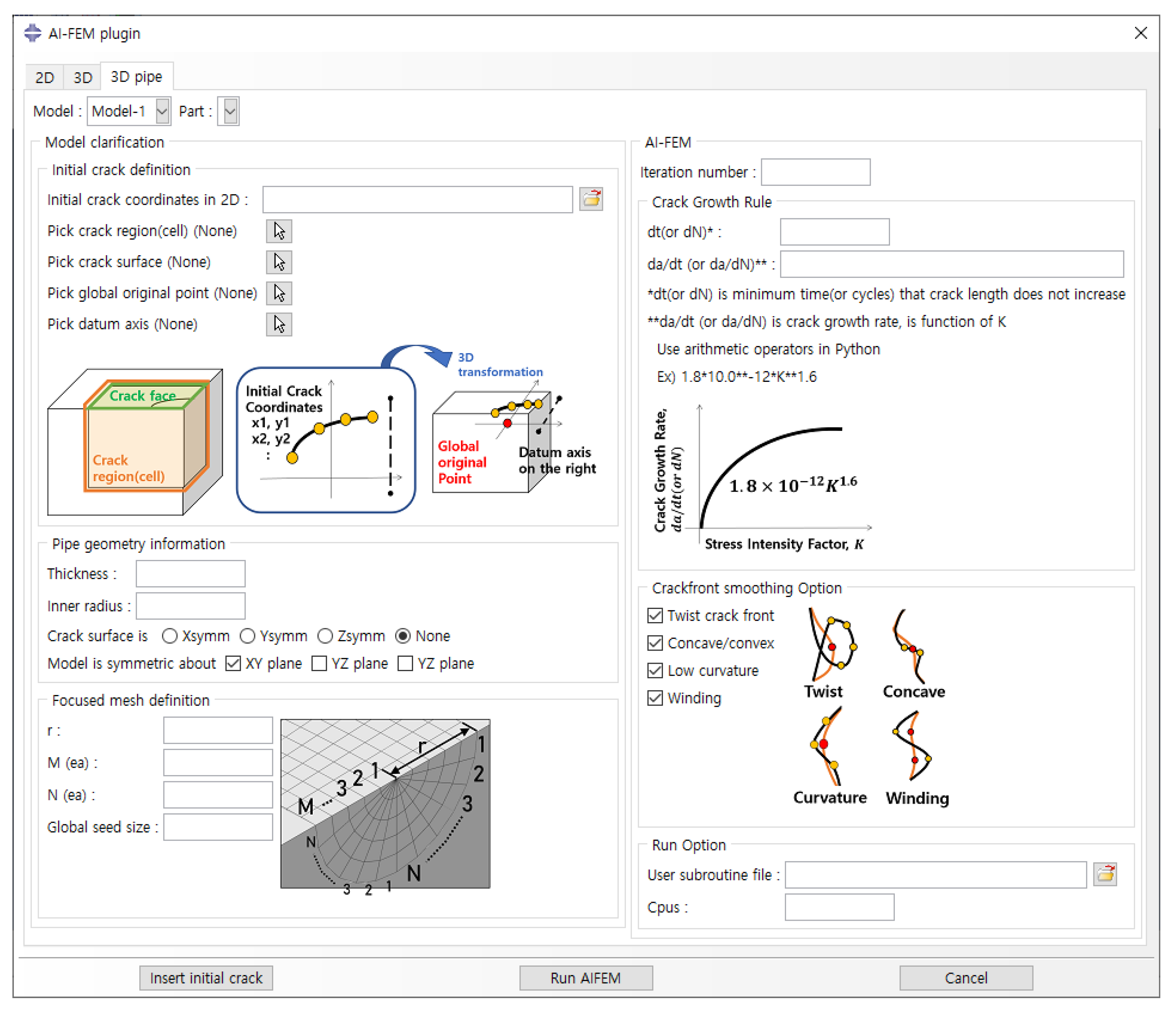
3.2. Defining the Structure and Crack Geometry

The first step in AI-FEM is to define the shape of the structure. This program can consider 2D/3D flat plate and 3D pipe models, and the shape can be determined from the upper menu of the GUI in Figure 8. Once the structure shape has been determined, the detailed characteristics of the structure and crack tip mesh should be defined. The submenus consist of pipe geometry information, model clarification, and focused mesh definition.

In the “Geometry information” category, the user can define the shape variables of the structure. For example, in the case of a 3D pipe, pipe thickness, inner radius, symmetry of shape, and location of crack surface are defined. In the “Model clarification” category, the user can define the characteristics of the initial crack. The crack can be inserted as a 1D crack in the 2D model and as a 2D crack in the 3D model, and the inserted crack is composed of a crack tip mesh. For the crack tip mesh, the crack region, crack surface, and crack coordinates are defined so that the crack can grow in an appropriate direction. In the “Focused mesh definition” category, detailed shape variables of the crack tip mesh such as the radius of the crack contour (r), the number of meshes within the radius (M), the number of meshes in the circumferential direction (N) and global seed size are defined. All variables can be entered as desired by the user and the efficient analysis can be performed by using the variables suggested in Table 4 in Section 2.2.6.

3.3. Defining the Crack Growth Characteristics

Once the structure and crack shape and crack tip mesh are determined, the crack growth characteristics must be defined, which can be determined through the submenu AI-FEM. AI-FEM consists of crack growth rule, crack front smoothing option, and run option.

In the “Crack growth rule” category, the relationship between SIF and crack growth rate is defined, and SCC growth and mechanical FCG can be simulated through this. The “Crack front smoothing option” category provides a function to compensate if the node arrangement of the grown crack tip is not suitable for the mesh for the next crack growth. The smoothing option is applied as default and can be turned off if not required. A description of the functions is as follows:

• Twist crack front: If crack propagation is large at a specific region in one cycle, normal directions at adjacent nodes may cross each other, which may cause twisting of the crack tip. This option helps to smooth the mesh of the crack tip by creating one node at the average point of the twisted node coordinates.
• Concave/convex: When the curvature between the nodes forming the crack tip is small, the two nodes are integrated to make the crack tip smooth.
• Low curvature: When nodes are concentrated in one area, the average point of the nodes within a certain distance is calculated and then combined into one node.
• Winding: If the curvature of the crack tip is repeated in an S-shape, the angle between the two points is relaxed.

Lastly, in the “Run option” category, the Abaqus user-subroutine file can be inserted, and additionally, stress fields such as residual stress in a structure can be mapped. The stress field is repeatedly inserted in every crack growth cycle.

4. Verification of AI-FEM

4.1. Comparison of SCC Growth with the ASME Method

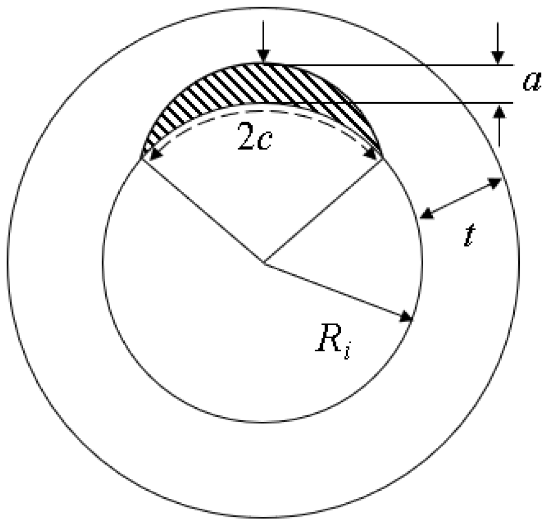
4.1.1. Geometry

In this section, to verify the reliability of AI-FEM, the SCC growth of a pipe with circumferential semi-elliptical inner surface crack was simulated, and the result was compared with the SCC growth calculation result using the method presented in ASME code, Sec. XI, App. C. Figure 9 shows schematics of the structure considered for verification. The inner radius (R_i) and thickness (t) of the pipe were 347.98 and 83.82 mm, respectively, and the various crack shapes in

Table 5. Shape variables of the cracks.

	a/t	a/c
Case 1	0.3	1
Case 2		1/2
Case 3		1/3
Case 4	0.5	1
Case 5		1/2
Case 6		1/3
Case 7	0.6	1

were considered.

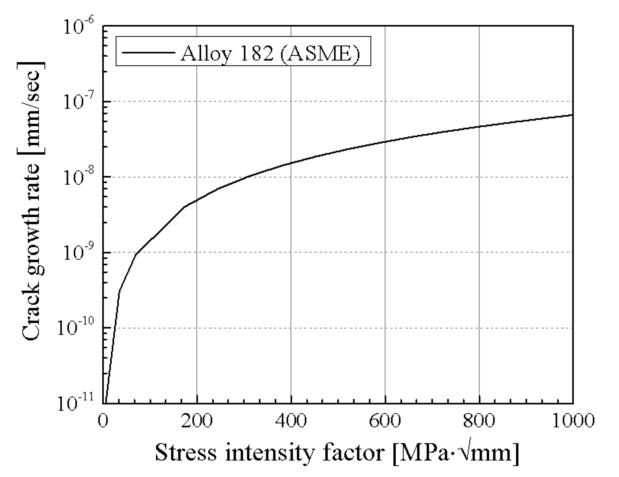
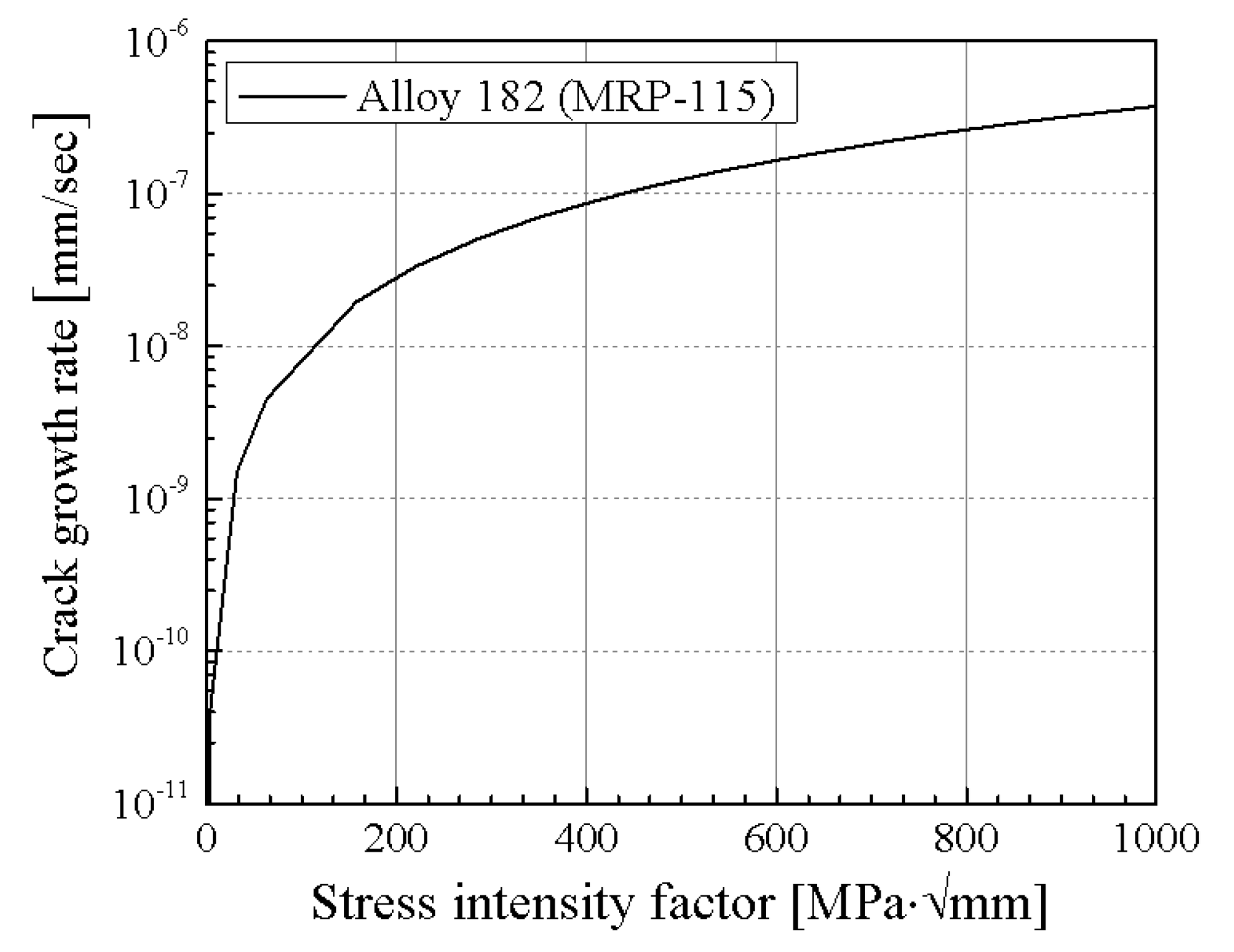
4.1.2. SCC Growth Law

The SCC growth rate curve for Alloy 182 in the pressurized water reactor (PWR) environment is presented in ASME code, Sec. XI, App. C was applied and is shown in Figure 10. The SCC growth curve for Alloy 182 is a function of the SIF and temperature, and the relation is as follows in Equation (2):

$$\frac{da}{dt}=\exp \left[-\frac{Q_g}{R_g}\left(\frac{1}{T_{abs}}-\frac{1}{T_{ref}}\right)\right]ø{\left(K_I-K_{Ith}\right)}^{\eta }$$

(2)

where K_I is the mode I SIF and K_Ith is the threshold value of the SIF. Q_g, R_g, T_abs, and T_ref are thermal activation energy for SCC growth, universal gas constant, absolute metal operating temperature, and absolute reference temperature for SCC, respectively. ø and η are the SCC growth factors. The values of each parameter are shown in

Table 6. Parameters of SCC growth.

KIth$\left[\mathbf{MPa}\sqrt{\mathbf{m}}\right]$	${\mathit{Q}}_{\mathit{g}}\left[\mathbf{kcal}/\mathbf{mole}\right]$	${\mathit{R}}_{\mathit{g}}\left[\mathbf{kcal}/\mathbf{mole}\text{-}\mathbf{R}\right]$	${\mathit{T}}_{\mathit{abs}}\left[°\mathbf{R}\right]$	${\mathit{T}}_{\mathit{ref}}\left[°\mathbf{R}\right]$	ø	η
0	31	1.103 × 10−3	1076.7	1009.67	0	1.6

. Also, the elastic modulus was considered to be 200 GPa, and the Poisson’s ratio was considered to be 0.3.

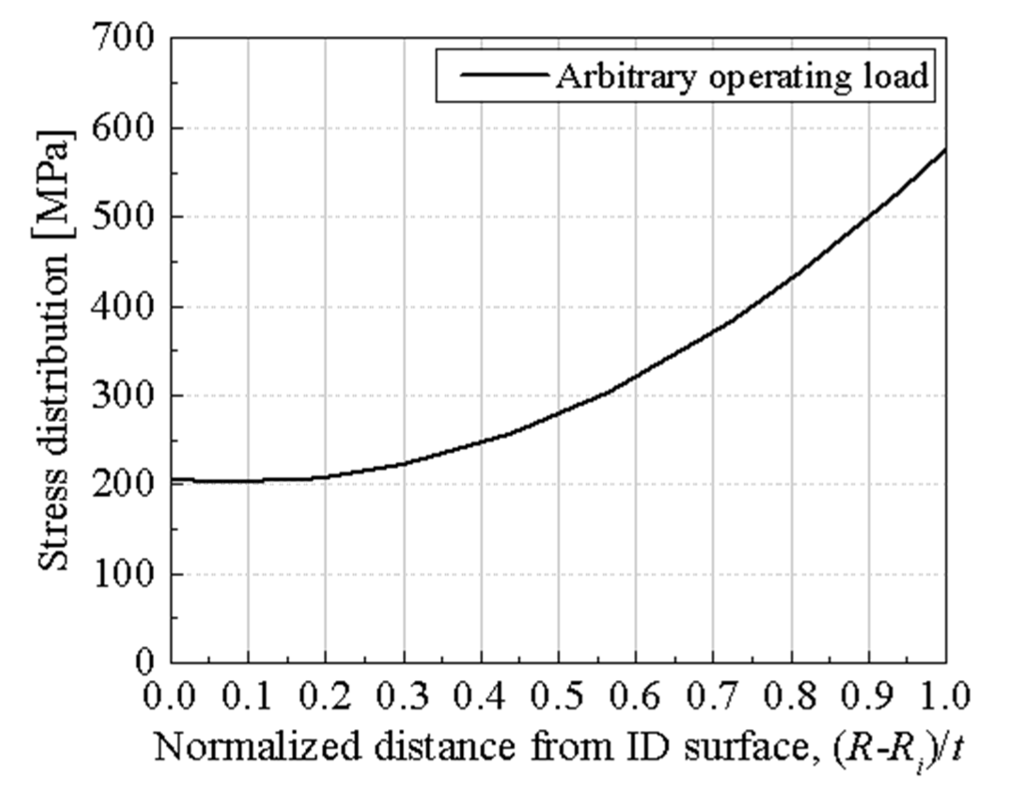
4.1.3. Loading Conditions

The load in Figure 11 was assumed to simulate SCC growth. The continuous load in one transient state was considered, and the load duration was set to about 1.5 years (13,140 h) in consideration of the inspection period during the operation of the nuclear power plant. The temperature when the load is applied was assumed to be 287.78 °C (550 °F), which is the operating temperature of the nuclear power plant.

4.1.4. SCC Growth Calculation Using ASME Code, Sec. XI

ASME code, Sec. XI, App. C provides cracked pipe evaluation methods and SCC growth rate relation according to the material. The method of calculating the SCC growth is as follows:

• Obtain the stress distribution in the pipe thickness direction by performing the thermal-structural coupling analysis of cracked pipe. This stress result is curve-fitted using the stress distribution formula of Equation (3) presented in ASME code, Sec. XI, App. A, A-3000.
• Calculate the SIF using the SIF formula of Equations (4) and (5) presented in ASME code, Sec. XI, App. A, A-3411 by applying the stress distribution formula.
• Calculate the crack growth rate for the corresponding SIF using the SCC growth rate calculation formula presented in ASME code, Sec. XI, App. C. When using this formula, if the crack growth cycle is defined largely, the SIF may change rapidly, and the crack growth rate may not be calculated accurately. Therefore, the crack growth cycle should be defined short enough in consideration of accuracy. (In this study, it was set to 100 h.)
• The crack size is updated by adding the calculated crack growth amount to the crack of the previous cycle.
• By repeating the above process until the load reaches the final cycle, the final crack size can be calculated.

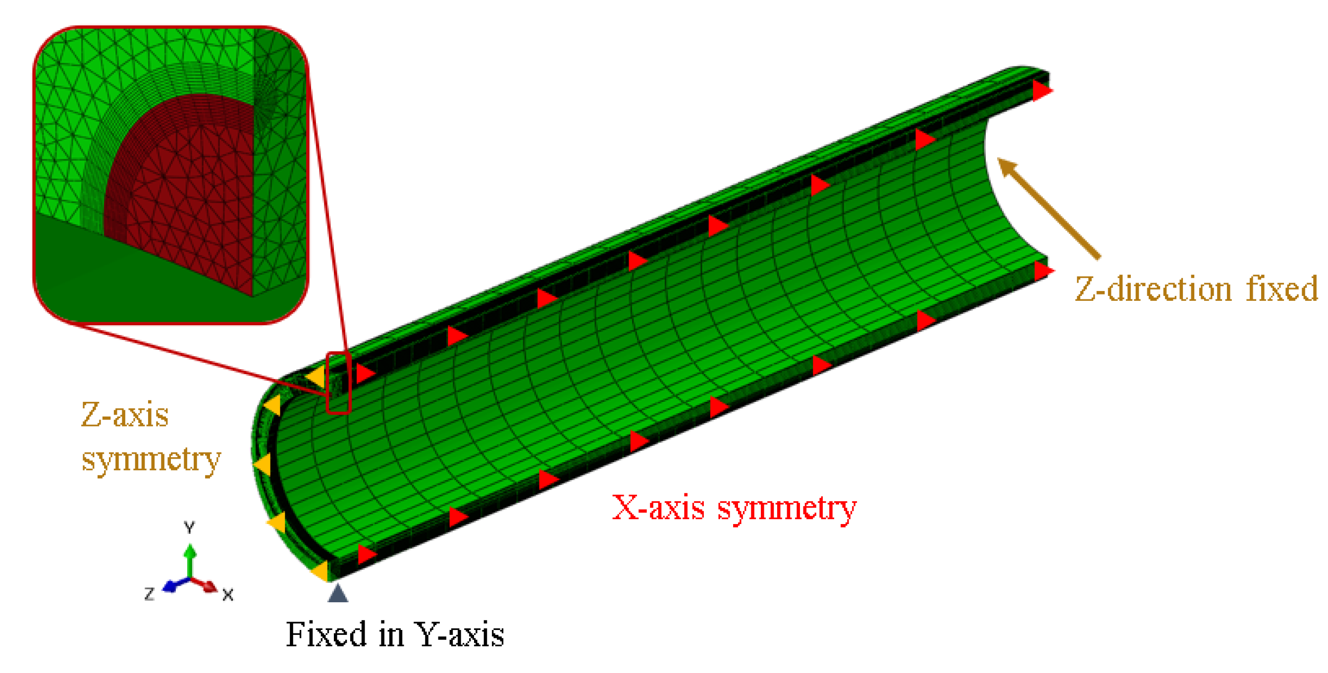
The stress distribution formula in the thickness direction is presented in ASME code, Sec. XI, App. A, A-3000 is as follows Equation (3):

$$\sigma =B_0+B_1\left(\frac{x}{t}\right)+B_2{\left(\frac{x}{t}\right)}^2+B_3{\left(\frac{x}{t}\right)}^3+B_4{\left(\frac{x}{t}\right)}^4$$

(3)

where, B₀~B₄ are the coefficients of a 4th-order polynomial, and these can be obtained by curve-fitting the stress distribution. By applying these coefficients to the SIF (K_I) formula of Equation (4) presented in ASME code, Sec. XI, App. A, A-3411, the SIF of a surface cracked pipe can be calculated.

$$K_I=\left[B_0{G}_0+B_1\left(\frac{x}{t}\right)G_1+B_2{\left(\frac{x}{t}\right)}^2{G}_2+B_3{\left(\frac{x}{t}\right)}^3{G}_3+B_4{\left(\frac{x}{t}\right)}^4{G}_4\right]\sqrt{\pi a/Q}$$

(4)

$$Q=1+4.593{\left(\frac{a}{l}\right)}^{1.65}-q_y$$

(5)

where G₁~G₄ are SIF coefficients that vary depending on the crack shape and are presented in the ASME code, Sec. XI as a table form. Q is the crack shape parameter and is shown in Equation (5). l is the crack length, a/l is the crack aspect ratio, q_y is the plastic region correction coefficient. To define crack growth, the SCC growth rate should be determined. From this, it is possible to calculate the final crack size due to SCC growth until the end of the loading period. In this section, the SCC growth rate of Alloy 182 is presented in ASME code, Sec. XI, App. C was used. The final crack size was calculated through the above procedure.

4.1.5. FE Model

To compare the final crack size calculated through the ASME method and AI-FEM, FE models were prepared as shown in Figure 12. The length of the pipe was set to 5 times the inner diameter to prevent the effect of the length. Considering the symmetry of the pipe and crack shape, the FE model was created as a 1/4 model. In order to obtain an accurate SIF value, a model was created by applying the guidelines suggested in Section 2.2. For the crack tip mesh, the shape variables determined in Section 2.2.6 were used, and the QUA and tied options were not applied. C3D20R element was applied as an element type. As a boundary condition, a symmetrical condition was applied to the symmetrical surface except for the crack surface, and one point was constrained in the Y-axis direction to avoid unnecessary movement of the pipe. Also, the end face of the pipe opposite to the crack surface restricted movement in the z-axis direction. The FE models were applied to the AI-FEM to calculate the final crack size.

4.1.6. Results

The final crack size at the end of the cycle calculated through the ASME method and AI-FEM were compared and shown in

Table 7. Comparison of SCC growth results.

		Initial	ASME (1.5 yr)	AI-FEM (1.5 yr)	Difference
Case 1	a [mm]	25.15	30.48	30.23	0.82%
	l [mm]	50.55	62.74	60.45	3.64%
Case 2	a [mm]	25.15	33.78	33.53	0.74%
	l [mm]	101.09	113.28	112.27	0.89%
Case 3	a [mm]	25.15	35.81	35.31	1.40%
	l [mm]	151.38	162.31	161.54	0.47%
Case 4	a [mm]	42.16	53.34	52.58	1.42%
	l [mm]	84.07	105.41	102.87	2.41%
Case 5	a [mm]	42.16	61.21	60.20	1.65%
	l [mm]	168.40	191.77	189.23	1.32%
Case 6	a [mm]	42.164	68.33	66.29	2.99%
	l [mm]	252.48	275.08	271.02	1.48%
Case 7	a [mm]	50.55	67.31	65.53	2.64%
	l [mm]	101.09	128.27	123.19	3.96%

. The difference in each crack growth result is defined in the following Equation (6):

$$Diff=\frac{G_{ASME}-G_{AI-FEM}}{G_{ASME}}$$

(6)

where, G_ASME represents the final crack size calculated through the ASME method, and G_AI-FEM represents the final crack size calculated through the AI-FEM. The difference in crack growth results according to the two methods was found to be a minimum of 0.42% and a maximum of 3.92%.

4.2. Comparison of Natural Crack Growth with AFEA Method including Cracking Transition

When a continuous load is applied to an inner surface crack and the crack growth continues, a transition to a through-wall crack may occur. Shim et al. [15] simulated natural crack growth using the AFEA method under PWSCC conditions considering various loads that may occur during operation. The cracking transition was also considered. In this section, the verification of AI-FEM was performed by comparing the crack growth results of AFEA and AI-FEM under the same conditions.

4.2.1. Cracking Transition Method

If the inner surface crack continues to grow in the thickness direction, it is converted into a through-wall crack, and a method for simulating the crack growth at the time of transition and after is needed for accurate soundness evaluation. In the MRP-216 [19] report, crack transition point is defined as when the deepest point of the crack reaches 93% of the pipe thickness, and in the Emc² report [14], the crack transition point is defined as the ligament is less than 5~10% of the pipe thickness. In this study, it was defined as when the deepest point of the crack reaches 95% of the pipe thickness.

For the external crack length after cracking transition, Shim et al. [23] applied the criterion of UK R6, and the relation is as follows Equation (7):

$$c_2=\min \left(t, \frac{c_1}{4}\right)$$

(7)

where t is the pipe thickness, c₁ is the length of the inner surface crack when the surface crack transitions into a through-wall crack, and c₂ is the length of the outer surface crack after the surface crack transitions into a through-wall crack. In this study, the cracking transition was simulated by applying the criteria of the crack length of R6.

4.2.2. Geometry

The shape of the pipe with semi-elliptical inner surface cracks considered in this verification is the same as the shape considered in Section 4.1 (Figure 9). The inner radius and thickness of the pipe are 150.368 mm and 40.132 mm, respectively, and the semi-elliptical crack has a depth of a = 10.434 mm and a length of l = 118.098 mm.

4.2.3. SCC Growth Law

In the MRP-115 report [24], crack growth curves for Alloy 182 in the SCC environment are presented and are shown in Figure 13. The relation is as follows in Equation (8):

$$\mathrm{CGR}\left(inm/s\right)=1.5\times {10}^{-12}{K}^{1.6}$$

(8)

where K is SIF and the crack growth length per cycle was calculated by applying the SIF calculated through AI-FEM to the above relation and the specified cycle. Also, the elastic modulus was considered to be 200 GPa, and the Poisson’s ratio was considered to be 0.3.

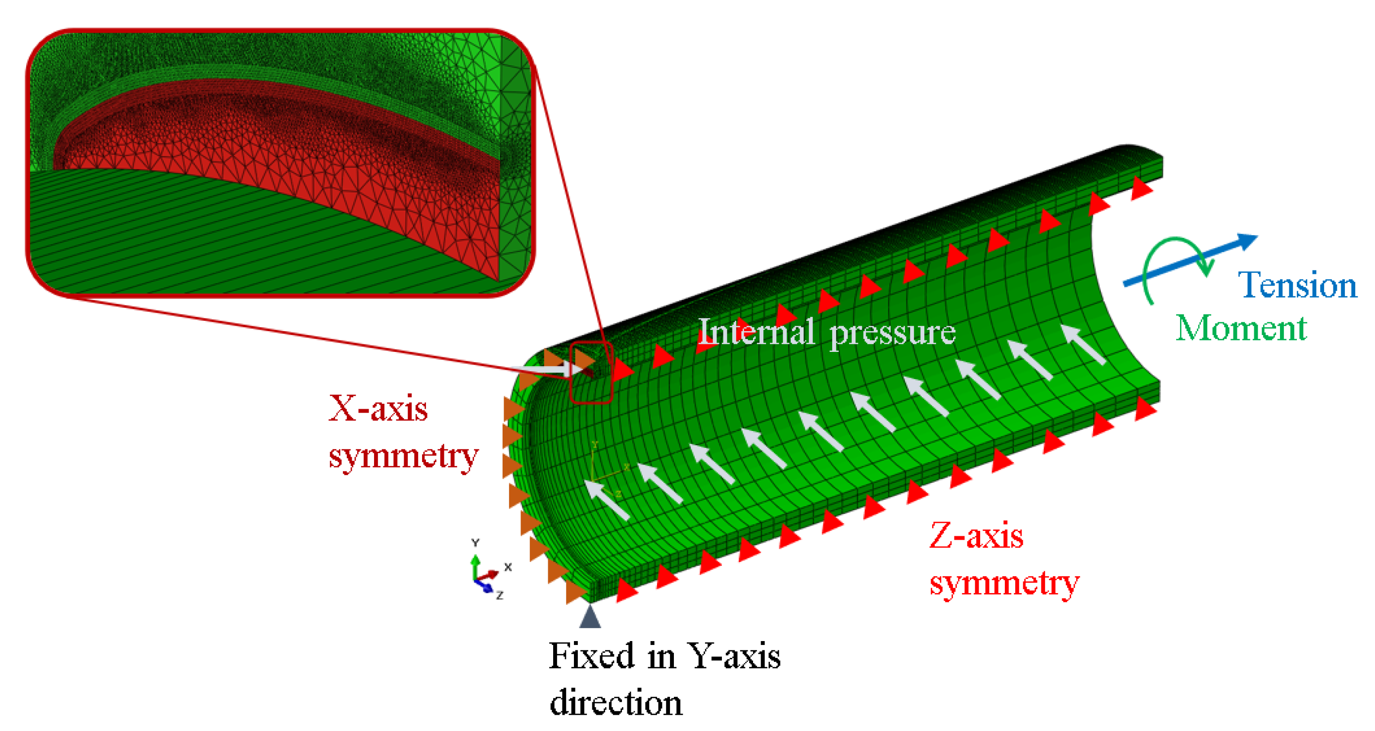
4.2.4. FE Model and Loading Conditions

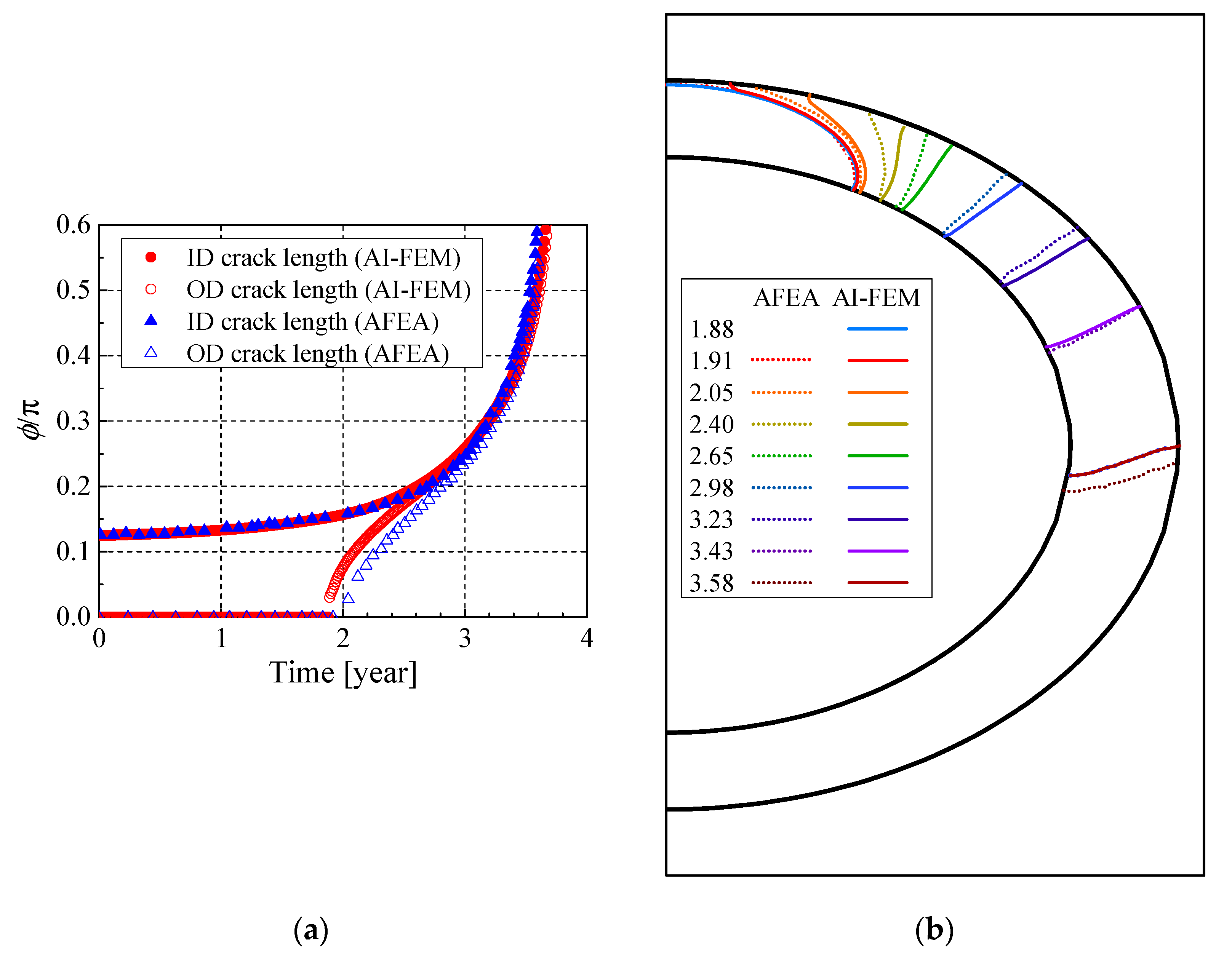
Figure 14 shows the FE model and loading conditions of a cracked pipe. The above guideline was applied when constructing the FE model, and it was composed of a 1/4 model for the efficiency of analysis. The operating loads considered in this study are shown in

Table 8. Loading conditions.

Internal Pressure [MPa]	Axial Tension [MPa]	Global Bending Moment [N mm]
15.41	27.58	1.62 × 108

.

4.2.5. Results

The results of natural crack growth performed by the AFEA method and AI-FEM were compared, as shown in Figure 15a. In both SCC growth results, the outer diameter (OD) crack length was 0 at first, and then showed a tendency to increase after a certain point, which means that the surface crack has transitioned to a through-wall crack. The results of SCC growth using the two methods showed good agreement with the inner surface behavior of cracks and showed a difference in the cracking behavior of the outer surface at the start of cracking transition and immediately thereafter. After sufficient crack propagation progressed, the crack behavior of the outer surface of the two has a similar trend, and the inner and outer crack lengths became almost the same. This trend can also be confirmed in Figure 15b, which directly compares the crack propagation shape in the pipe section. These results show that AI-FEM can reasonably simulate cracking transition compared to existing studies.

5. Conclusions

In this study, AI-FEM, a program that operates as a plug-in of Abaqus, a commercial FEA program, was developed. AI-FEM is a program that performs automatic crack growth based on FEA for natural crack. This program can simulate FCG and SCC growth for various structures including 2D/3D plates and pipes. In addition, loads such as internal pressure, bending and tensile loads, and residual stresses, which are generally considered in NPP components, can be applied.

Sensitivity analysis was performed on various variables affecting accurate SIF calculation, such as SIF calculation method, element type, shape, variables of crack tip-mesh, and crack growth characteristics, and analysis results of each variable were compared with the Raju-Newman solution. Through this, default settings and guidelines for the program were provided.

To ensure the reliability of AI-FEM, two verifications were performed. First, the same SCC growth was simulated using AI-FEM and fracture mechanics evaluation method presented by ASME code, Sec. XI, App. C, and the results were compared. These two methods showed a difference of a minimum of 0.42% and a maximum of 3.92% in the final crack size, and it was confirmed that the two results showed good agreement. Second, SCC growth of natural cracks was performed by applying AI-FEM and AFEA methods, and the results were compared. In this process, the cracking transition from surface crack to through-wall crack was considered. Although the two methods showed some differences in the crack behavior of the outer surface at the moment of cracking transition and immediately after, it was confirmed that the crack behavior of both the inner and outer surfaces coincided well after cracking progressed.

From the results of two verification cases, it was confirmed that AI-FEM simulates crack growth in a structure accurately, and especially, it was confirmed that crack growth including cracking transition can be simulated well. Therefore, it is concluded that using AI-FEM with automatic re-meshing function can quickly and accurately calculate the SIF even when the crack shape is complicated, and can simulate the crack growth behavior accurately.

References

1. Terachi, T.; Yamada, T.; Miyamoto, T.; Arioka, K. SCC growth behaviors of austenitic stainless steels in simulated PWR primary water. J. Nucl. Mater. 2012, 426, 59–70. [Google Scholar] [CrossRef]
2. Sullivan, E.J.; Anderson, M.T. Assessment of Weld Overlays for Mitigating Primary Water Stress Corrosion Cracking at Nickel Alloy Butt Welds in Piping Systems Approved for Leak-before-Break; No. PNNL-21660; Pacific Northwest National Lab. (PNNL): Richland, WA, USA, 2012. [Google Scholar]
3. King, C.; Frederick, G. Technical Basis for Preemptive Weld Overlays for Alloy 82/182 Butt Welds in PWRs (MRP-169); EPRI Topical Report; Electric Power Research Institute: Palo Alto, CA, USA, 2005; p. 1012843. [Google Scholar]
4. Kamaya, M. Growth evaluation of multiple interacting surface cracks. Part I: Experiments and simulation of coalesced crack. Eng. Fract. Mech. 2008, 75, 1336–1349. [Google Scholar] [CrossRef]
5. White, G.; Broussard, J.; Collin, J.; Klug, M.; Harrington, C.; DeBoo, G. Advanced FEA modeling of PWSCC crack growth in PWR dissimilar metal piping butt welds and application to the industry inspection and mitigation program. In Proceedings of the ASME Pressure Vessels and Piping Conference, Chicago, IL, USA, 27–31 July 2008; Volume 48296. [Google Scholar]
6. Chen, X.; Chen, X.; Chan, A.; Cheng, Y.; Wang, H. A FDEM parametric investigation on the impact fracture of monolithic glass. Buildings 2022, 12, 271. [Google Scholar] [CrossRef]
7. Chen, X.; Luo, T.; Ooi, E.T.; Ooi, E.H.; Song, C. A quadtree-polygon-based scaled boundary finite element method for crack propagation modeling in functionally graded materials. Theor. Appl. Fract. Mech. 2018, 94, 120–133. [Google Scholar] [CrossRef]
8. Chen, X.; Chan, A.H. Modelling impact fracture and fragmentation of laminated glass using the combined finite-discrete element method. Int. J. Impact Eng. 2018, 112, 15–29. [Google Scholar] [CrossRef]
9. Nguyen, T.T.; Yvonnet, J.; Zhu, Q.Z.; Bornert, M.; Chateau, C. A phase-field method for computational modeling of interfacial damage interacting with crack propagation in realistic microstructures obtained by microtomography. Comput. Meth. Appl. Mech. Eng. 2016, 312, 567–595. [Google Scholar] [CrossRef] [Green Version]
10. Rezaei, S.; Mianroodi, J.R.; Brepols, T.; Reese, S. Direction-dependent fracture in solids: Atomistically calibrated phase-field and cohesive zone model. J. Mech. Phys. Solids. 2021, 147, 104253. [Google Scholar] [CrossRef]
11. Rezaei, S.; Harandi, A.; Brepols, T.; Reese, S. An anisotropic cohesive fracture model: Advantages and limitations of length-scale insensitive phase-field damage models. Eng. Fract. Mech. 2022, 261, 108177. [Google Scholar] [CrossRef]
12. Gao, Y.; Liu, Z.; Wang, T.; Zeng, Q.; Li, X.; Zhuang, Z. XFEM modeling for curved fracture in the anisotropic fracture toughness medium. Comput. Mech. 2019, 63, 869–883. [Google Scholar] [CrossRef]
13. Hou, J.; Goldstraw, M.; Maan, S.; Knop, M. An Evaluation of 3D Crack Growth Using ZENCRACK. ACK. Defense Science and Technology Organization; Report Number: DSTO-TR-1158; Department of Defence: Melbourne, Australia, 2001. [Google Scholar]
14. Rudland, D.L.; Shim, D.J.; Zhang, T.; Wilkowski, G. Implications of Wolf Creek Indications—Final Report, Program Final Report to the NRC; ADAMS File Number ML072470394; Engineering Mechanics Corporation of Columbus: Columbus, OH, USA, 2007. [Google Scholar]
15. Shim, D.J.; Rudland, D.; Harris, D. Modeling of subcritical crack growth due to stress corrosion cracking: Transition from surface crack to through-wall crack. In Proceedings of the 2011 ASME Pressure Vessels and Piping Conference, Baltimore, MD, USA, 17–21 July 2011; Volume 44564. [Google Scholar]
16. Nakamura, H.; Tajima, S.; Hazama, O.; Gu, W. Automated fracture mechanics and fatigue analyses based on three-dimensional finite element for welding components. In Proceedings of the ASME 2014 Pressure Vessels and Piping Conference, Anaheim, CA, USA, 20–24 July 2014; Volume 45998. [Google Scholar]
17. Nakamura, H.; Matsushima, E.; Okamoto, A.; Umemoto, T. Fatigue crack growth under residual stress field in low-carbon steel. Nucl. Eng. Des. 1986, 94, 241–247. [Google Scholar] [CrossRef]
18. Ogawa, T.; Itatani, M.; Hayashi, T.; Saito, T. SCC growth prediction for surface crack in welded joint using advanced FEA. In Proceedings of the 2020 ASME Pressure Vessels and Piping Conference, Virtual, 3 August 2020; Volume 83860. [Google Scholar]
19. Materials Reliability Program: Advanced FEA Evaluation of Growth of Postulated Circumferential PWSCC Flaws in Pressurizer Nozzle Dissimilar Metal Welds; MRP-216, Rev. 1; EPRI: Palo Alto, CA, USA, 2007.
20. Dassault Systemes Corp. ABAQUS/Standard User’s Manuals; Ver. 2020; Dassault Systèmes SE: Vélizy-Villacoublay, France, 2020. [Google Scholar]
21. Anderson, T.L. Fracture Mechanics: Fundamentals and Applications; CRC Press: Boca Raton, FL, USA, 2003. [Google Scholar]
22. Raju, I.S.; Newman, J.C. Stress-intensity factors for a wide lange of semi-elliptical surface cracks in finite-thickness plates. Eng. Fract. Mech. 1979, 11, 817–829. [Google Scholar] [CrossRef]
23. Shim, D.J.; Kurth, R.; Rudland, D. Development of non-idealized surface to through-wall crack transition model. In Proceedings of the 2013 ASME Pressure Vessels and Piping Conference, Paris, France, 14–18 July 2013; Volume 55706. [Google Scholar]
24. Materials Reliability Program: Crack Growth Rates for Evaluating Primary Water Stress Corrosion Cracking (PWSCC) of Alloy 82, 182, and 132 Welds; EPRI: Palo Alto, CA, USA, 2004.
Figure 1. The procedure of the crack growth analysis in AI-FEM.
Applsci 12 03075 g001
Figure 2. Structural schematics considered in crack tip meshing strategies: (a) A flat plate with a surface crack; (b) Shape parameters of semi-elliptical surface crack.
Applsci 12 03075 g002
Figure 3. FE model of a flat plate with semi-elliptical crack: (a) Boundary and loading condition; (b) Detailed crack tip mesh and shape variables.
Applsci 12 03075 g003
Figure 4. Comparison of SIF according to calculation methods [22].
Applsci 12 03075 g004
Figure 5. Comparison of SIF according to element types [22].
Applsci 12 03075 g005
Figure 6. Comparison of SIF according to crack tip element characteristics [22].
Applsci 12 03075 g006
Figure 7. Comparison of SIFs according to crack tip mesh shape variables: (a) The number of elements in the radial direction of the contour (M); (b) The ratio of the relative contour size to the crack size (r/x); (c) The number of elements in the circumferential direction inside the contour (N); (d) The ratio of the total length of the crack tip to the radial size of the element (AR) [22].
Applsci 12 03075 g007
Figure 8. The graphical user interface of AI-FEM.
Applsci 12 03075 g008
Figure 9. Schematics of pipe with circumferential semi-elliptical inner surface crack.
Applsci 12 03075 g009
Figure 10. SCC growth rate curve for Alloy 182 presented in ASME code, Sec. XI.
Applsci 12 03075 g010
Figure 11. Stress distribution in the thickness direction applied to the pipe.
Applsci 12 03075 g011
Figure 12. FE model and boundary conditions of a pipe with semi-elliptical surface crack.
Applsci 12 03075 g012
Figure 13. SCC growth rate curve for Alloy 182 presented in MRP-115.
Applsci 12 03075 g013
Figure 14. FE model and boundary conditions of cracked pipe used for verification.
Applsci 12 03075 g014
Figure 15. Comparison of SCC growth results according to time change: (a) Crack angles on inner and outer surfaces; (b) Overall crack shapes.
Applsci 12 03075 g015