Photoluminescence of Cis-Polyacetylene Semiconductor Material

Abstract

Photoluminescence (PL) is one of the key experimental characterizations of optoelectronic materials, including conjugated polymers (CPs). In this study, a simplified model of an undoped cis-polyacetylene (cis-PA) oligomer was selected and used to explain the mechanism of photoluminescence (PL) of the CPs. Using a combination of the ab initio electronic structure and a time-dependent density matrix methodology, the photo-induced time-dependent excited state dynamics were computed. We explored the phonon-induced relaxation of the photoexcited state for a single oligomer of cis-PA. Here, the dissipative Redfield equation of the motion was used to compute the dissipative excited state dynamics of electronic degrees of freedom. This equation used the nonadiabatic couplings as parameters. The computed excited state dynamics showed that the relaxation rate of the electron is faster than the relaxation rate of the hole. The dissipative excited-state dynamics were combined with radiative recombination channels to predict the PL spectrum. The simulated results showed that the absorption and emission spectra both have a similar transition. The main result is that the computed PL spectrum demonstrates two mechanisms of light emission originating from (i) the inter-band transitions, corresponding to the same range of transition energies as the absorption spectrum and (ii) intra-band transitions not available in the absorption spectra. However, the dissipative Redfield equation of the motion was used to compute the electronic degrees of freedom of the nonadiabatic couplings, which helped to process the time propagation of the excited dynamic state. This excited dynamic state shows that the relaxation rate of the electron is faster than the relaxation rate of the hole, which can be used for improving organic semiconductor materials for photovoltaic and LED applications.

1. Introduction

Over the past few years, conjugated oligomers and polymers have attracted considerable attention due to their applications in photovoltaic cells, light-emitting diodes (LEDs), field-effect transistors (FETs), electrochromic devices, chemical sensors, microelectronic actuators, etc. [1,2]. A large amount of experimental and computational work has been devoted to studying the electronic properties of conjugated polymers using density functional theory (DFT) by means of approximate values of energy and state density. However, this type of research is quite complicated because the polymers do not have a well-defined structure, many of them are insoluble and polydisperse, and there are far fewer computational techniques for infinite polymers than well-defined molecules.

In recent years, DFT has gradually replaced semiempirical methods, Hartree–Fock (HF) theory and perturbation theory in research on conjugated oligomers and polymers. Despite the many successes of DFT, HF theory gives a better approximation of the electronic properties of the CPs. To understand the behavior of the ground state of the electron and the interface of the material via photo-induced charge transfer, it is important to study CPs using DFT and nonadiabatic coupling calculations. To explore the electronic structure of the CPs, ab initio DFT molecular dynamic simulation can be studied in combination with quantum dynamic calculations of the electronic relaxation to investigate the electron transfer of CPs. For example, Han et al. [3] studied the photo-induced charge transfer of an Au/Si metal-semiconductor nano-interface through a reduced density matrix (RDM), which was explained via Redfield theory and nonadiabatic coupling calculations based on the ab initio equations of a density function. The nonadiabatic couplings between electronic orbitals were processed on the fly along nuclear trajectories of the system [3].

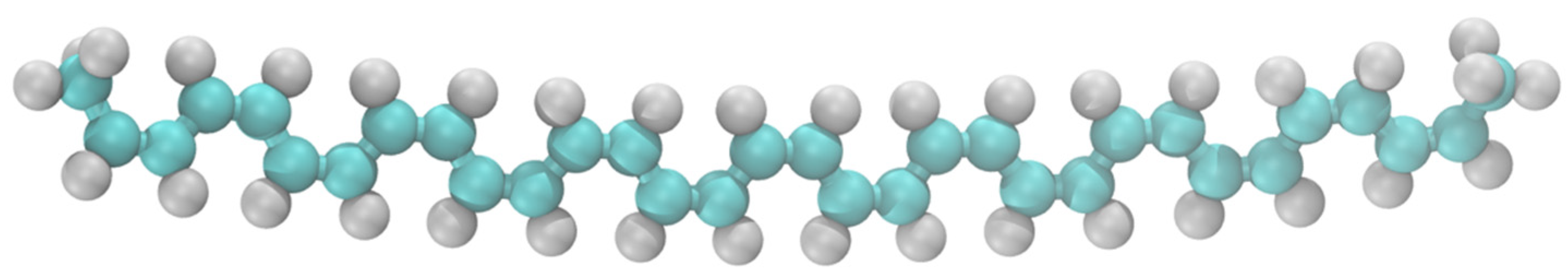
In this study, we considered a model of a polyacetylene (PA) which has no commercial use yet, although PA is used as a processing solution for film-forming conductive polymers and molecular electrons. PA polymers are one of the commonly used polymers for photovoltaics, LEDs (light-emitting diodes), diodes, and transistors; in these applications, one needs to design and operate materials with modified electronic properties [3]. Therefore, electronic properties can be modified by using different types of approaches such as changing the composition of the polymer by adding doping, photoexcitation, or an injected charge, which occurs after applying different kinds of processes, such as photoexcitation, injection of charge, thermal motion (e.g., glass transition) or tight packing in the amorphous form of the material [4]. During the last few decades, many researchers have worked on the electronic conductivity of polyacetylene, and it has received much attention among them, particularly because of the possibility of increasing its electronic conductivity by doping and the low dimensionality of the electrical conductivity [5]. In 1977, for the first time, researchers published a study on the electrical conductivity of doped polyacetylene [6]. Recently, Carter et al. [7] explained the electronic and physical properties of trans-polyacetylene. In that article, they explained the infrared photoluminescence of PA which was used to study the electronic structure of PA. They concluded that the photogenerated excitons that were generated at or near cis defects could become trapped at the cis (—CH=CH—) bond and undergo radiative recombination [7]. The observed photoluminescence emission energies were a function of the conjugation length of the cis defect and the extent of local interchain π stacking. They proved that the cis bond served to pinpoint and localize the photogenerated excitons formed on the polyacetylene chain [7]. Analysis of the integrated photoluminescence intensities indicated that the percolation threshold for free carriers was achieved at just 30% overall trans content, implying that thermally isomerized polyacetylene behaved more like a three-dimensional composite material than a one-dimensional material [7]. Wong et al. [8] explored the emission properties of cis- and trans-polyacetylene, which was controlled by the ratio of cis- and trans-polymers. They found that the emission efficiency and PL lifetime decreased with an increase in cis content. Yoshino et al. explained the characterization of PL (photoluminescence) and EL (electroluminescence) by using polyacetylene derivatives. They experimentally proved that intensity of PL and the spectrum were dependent on the PA and various electrode configurations [9]. Hidayat et al. studied the PL and EL of the mixtures of PA and found a remarkable spectral shift in PL and EL [10]. Franco et al. [11] studied the computational examination of trans-polyacetylene oligomers, which was based on the electron vibrational dynamics of molecular systems. Flick et al. [12] investigated the nonadiabatic contributions to the vibronic sidebands of equilibrium and explicitly time-resolved nonequilibrium photoelectron spectra for a vibronic model system of trans-polyacetylene. They explained how the vibronic wavepacket motion of the model could be located in the time-resolved photoelectron spectra as a function of the pump–probe delay. Moliton et al. [13] explained that after modification, π-conjugated polymers such as PA could be used for optoelectronics applications. Because of electronic correlation effects and strong electron–phonon interactions, the theoretical description of π-conjugated polymers is very complicated. From the previous studies on polyacetylene, it can be understood that [14,15] that coupling of the electrons to the nuclear degrees of freedom results depends on the semiconductor or crystalline metal materials of the PA. Tretiak et al. [16] observed strong coupling to the nuclear degrees of freedom of the excited state electron nuclear dynamics of a polyacetylene chain. They explained the photoexcitation dynamics of conjugated cis-polyacetylene oligomers using an ESMD quantum chemical approach, and found that the excitation moves to the lowest electronic energy and creates phonon excitations and significant local distortions towards the lattice. Gal et al. [17] made a polymer using polyacetylene and experimentally proved that the polymer, which was prepared from polyacetylene, showed higher (352 nm) UV–visible absorption characteristics, and its highest photoluminescence spectrum was at 453 nm, which corresponds to the photon energy of 2.74 eV. Kim et al. [18] reported the synthesis and properties of a new polyacetylene-based polyelectrolyte. The absorption spectrum exhibited a maximum absorption value of 480 nm, which was due to the p→p* transition of the conjugated polymer backbone. The photoluminescence spectra of the polymer exhibited a maximum peak of 550 nm, which corresponded to a photon energy of 2.26 eV. Typical irreversible electrochemical behaviors were observed between the doped and undoped peaks in the cyclic voltammograms of the polymer.

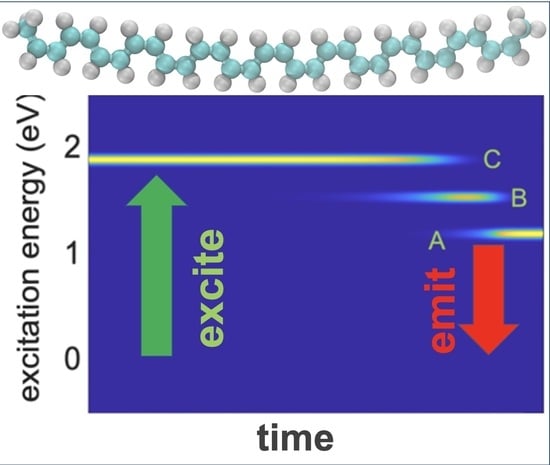
In this study, we have considered a simple single oligomer model of cis-polyacetylene to investigate interfacial electron transfer in the system, and representative nuclear configurations were obtained according to ab initio DFT molecular dynamic simulations and the time-dependent electronic structure. We considered the relaxation rates of photoexcited electrons and holes for our simulation using ab initio treatment of the electronic states when the underlying nonadiabatic transitions are accompanied by the respective vibrational dynamics. For this calculation, we used the Redfield theory for the calculation of the on-the-fly nonadiabatic couplings. which provide the dynamics of carriers and allow for an analysis of multiple nonradiative relaxation pathways in the cis-polyacetylene’s single oligomer. Photoexcitation can be found in this model by calculating the electron−phonon dynamics. In this work, we simulated our model using time-resolved emission spectra of the cis-polyacetylene, which provided some information about the lifetime of the emission state of the model. Our simulated results were only used for analyzing the thermal fluctuations of the lattice ions through nonadiabatic couplings, showing that for selected photoexcitations, the electron is promoted from carbon to hydrogen in the photon-mediated process and then recombines with the ground state calculation.

2. Methods

In this study, theoretical methods were cogently structured into two sections: ground-state DFT and nonadiabatic molecular dynamic calculations.

This section is divided into subheadings. This should provide a concise and precise description of the experimental results and their interpretation, as well as the experimental conclusions that can be drawn.

2.1. Ground-State DFT

In this research work, the atomic model was defined by the initial positions of each ion ${\overrightarrow{R}}_I$. The electronic structure was calculated through the solution of a self-consistent equation of DFT [19] via the Vienna Ab initio Simulation Package (VASP) [20]. This approach is based on a fictitious one-electron Kohn−Sham (KS) equation [21]. Kohn–Sham equations are used in a self-consistent DFT procedure to get a better approximation of the orbital energy.

$$\left(-\frac{{\hslash }^2}{2m}{\nabla }^2+v[\{{\overrightarrow{R}}_I\},\overrightarrow{r,}\rho (\overrightarrow{r})]\right){\phi }_i^{KS}(\{{\overrightarrow{R}}_I\},\overrightarrow{r})={\epsilon }_i(\{{\overrightarrow{R}}_I\}){\phi }_i^{KS}(\{{\overrightarrow{R}}_I\},\overrightarrow{r})$$

(1)

where the first term $T$ corresponds to kinetic energy and uses the symbol of gradient $\nabla =\left(\frac{\partial }{\partial x},\frac{\partial }{\partial y},\frac{\partial }{\partial z}\right)$. In Equation (1), we find a set of one-electron orbitals ${\phi }_i^{KS}\left(r\right),$ and their energies ${\epsilon }_i$. The orbitals are combined with the orbital occupation function $f_i$ for constructing the total density of electrons as:

$$\rho \left(\overrightarrow{r}\right)={\displaystyle \sum }_i{f}_i{\phi }_i^{K{S}^{*}}\left(\overrightarrow{r}\right){\phi }_i^{KS}\left(\overrightarrow{r}\right)$$

(2)

The total density defines the potential:

$$v\left[ \overrightarrow{r}, \rho \right]=\delta \left(E^{tot}\left[\rho \right]-T\left[\rho \right]\right)/\delta \rho$$

(3)

The potential energy is defined in terms of a functional derivative of the total energy with respect to the variation in the total density and includes the interactions of electrons with ions, and three electron interactions: Coulomb, correlation and exchange. Rectangular brackets indicate functions. Equations (1)–(3) are solved in the iterative, self-consistent manner by using hybrid functionals, which gives us approximate exchange correlation results.

In this article, HSE (Heyd–Scuseria–Ernzerhof) functions were used to improve the computational efficiency of the systems. The HSE function calculated from the fraction of Fock exchange, $a$, at zero electron separation and a length scale, ${\omega }^{-1}$, where the short-range Fock exchange is computed as follows [22]:

$$E_{Xc}^{HSE}=a{E}_X^{HF, SR}\left(\omega \right)+\left(1-a\right)E_X^{PBE, SR}\left(\omega \right)+E_X^{PBE, LR}\left(\omega \right)+E_c^{PBE}\left(\omega \right)$$

(4)

where $E_X^{HF, SR}\left(\omega \right)$ is the component of the Hartree–Fock exact exchange function; $E_X^{PBE, LR}\left(\omega \right)$ and $E_X^{PBE, SR}\left(\omega \right)$ are the long- and short-range elements of the PBE (Perdew–Burke–Ernzerhof) exchange function, and $E_c^{PBE}\left(\omega \right)$ is used to compute the correlation of the PBE function. In the above, $E_X^{HF, SR}\left(\omega \right)$ is computed through the spinful Kohn−Sham density matrix $\rho \sigma ,{\sigma }^{\prime }\left(r,r^{\prime }\right)$, which is given below:

$$E_X^{HF,SR}\left(\omega \right)=-\frac{1}{2}{\displaystyle \sum }_{\sigma ,{\sigma }^{\prime }}{\displaystyle \int }dr dr\prime \frac{erfc\left( \omega \left|r-r^{\prime }\right|\right)}{\left|r-r^{\prime }\right|}\times {\left|\rho \sigma ,{\sigma }^{\prime }\left(r,r^{\prime }\right)\right|}^2$$

(5)

Though this function’s accuracy was equal to PBE0, the value of $a=0.25$ for the exchange fraction was limited. Therefore, for improving the accuracy, we reparametrized the HSE06 function, which was based on $\omega$ not $a$ [23,24].

The density of states for all orbitals $n\left(\epsilon \right)$ and for occupied orbitals $n^{\prime }\left(\epsilon \right)$ can be expressed in the following equations:

$$n\left(\epsilon \right)={\displaystyle \sum }_i\delta \left(\epsilon -{\epsilon }_i\right)$$

(6)

$$n^{\prime }\left(\epsilon \right)={\displaystyle \sum }_i{f}_i\delta \left(\epsilon -{\epsilon }_i\right)$$

(7)

where ${\epsilon }_i$ is the KS energy of a given orbital, and the index i corresponds to each orbital calculated by using DFT.

In what follows, one uses the following definitions: $i \le HOMO, \mathrm{for} f_i \le \frac{1}{2}$ for the valence band, while $i \ge LUMO, f_i \ge \frac{1}{2}$ for the conduction band. The bandgap is defined as $band gap=\left|{\epsilon }_{LUMO}-{\epsilon }_{HOMO}\right|$. In Equation (4), $\delta \left(\epsilon -{\epsilon }_i\right)$ is the Dirac delta function, modeled by a Lorentzian function:

$$\delta \left(x\right)=\frac{1}{\pi }\frac{\sigma }{{\sigma }^2+x^2}$$

(8)

where σ is a parameter and the Delta function, both parameters have the same dimensions, which gives the width of the distribution. The value $\sigma =0.05 \mathrm{eV}$ was used to simulate spectral line broadening in an experimental measure of the density of states. The absorption spectrum can be expressed as:

$$a\left(\epsilon \right)={\displaystyle \sum }_{ij}{f}_{ij}\delta \left(\epsilon -\mathsf{\Delta }{\epsilon }_{ij}\right)$$

(9)

where $f_{ij}$ is the oscillator strength which describes the transition probability from the initial state i to the final state j, and is defined as:

$$f_{ij}={\left|{\overrightarrow{D}}_{ij}\right|}^2\frac{4\pi m_e{v}_{ij}}{3\underset{\_}{h}{e}^2}$$

(10)

in which $m_e$ is the mass of an electron, $\hslash$ is Planck’s reduced constant, $v_{ij}$ is the resonant frequency, $e$ is the charge of the electron and ${\overrightarrow{D}}_{ij}$ is the electric dipole moment matrix element for the transition between the initial state $i$ and the final state $j$. ${\overrightarrow{D}}_{ij}$ is expressed as:

$${\overrightarrow{D}}_{ij}=e\int {\phi }_i^{K{S}^{*}}\overrightarrow{r}{\phi }_j^{KS}d\overrightarrow{r}$$

(11)

This uses the summation of the positions of all electrons in the system ($\overrightarrow{r}$) and the elementary charge $e.$ The electronic structure of atomic models was explored with an equilibrium-optimized geometry and along the nuclear trajectory $\{{\overrightarrow{R}}_I\left(t\right)\}$ modeling system interfacing a thermostat. The positions of ions are entered into the DFT equations as parameters, as in Equation (1).

The orbitals computed by Equation (1) are visualized and interpreted in the form of 3D iso-surfaces of partial charge density, for a selected orbital ${\left|{\phi }_i^{KS}\left(\overrightarrow{r}\right)\right|}^2$ or by 1D distributions:

$${\rho }_i\left(z\right)=\iint dxdy{\left|{\phi }_i^{KS}\left(x,y,z\right)\right|}^2$$

(12)

$${\rho }_i\left(y\right)=\iint dxdz{\left|{\phi }_i^{KS}\left(x,y,z\right)\right|}^2$$

(13)

2.2. Nonadiabatic Calculations

In this current study, nonadiabatic calculations were used to understand the charge transfer of the system. Currents and electronic densities can be obtained using RDM (reduced density matrix) elements ${\rho }_{jk}$, where $j$ and $k$ are the electronic orbitals. All the calculations formed here are based on Kohn–Sham (KS) orbitals, which were used for DFT calculations. We used ab initio molecular dynamics (MD) to compute the nonadiabatic coupling of the system, which provided dissipative transitions. Electronic dissipative transitions ${\left(\frac{d{\rho }_{jk}}{dt}\right)}_{diss}$ were computed along a molecular dynamic trajectory for the positions of ions $\{{\overrightarrow{R}}_I\left(t\right)\}$ with the initial conditions for the positions $\{{\overrightarrow{R}}_I\left(t=0\right)\}$ and velocities $\left\{\frac{d}{dt}{\overrightarrow{R}}_I\left(t=0\right)\right\}$ representing ambient temperature. Along with the nuclear trajectory, the nonadiabatic couplings of the system can be computed as follows [24,25]:

$$V_{ij}\left(t\right)=\frac{-i\hslash }{\mathsf{\Delta }t}\int d\overrightarrow{r} {\phi }_i^{KS*}\left( \left\{{\overrightarrow{R}}_I\left(t\right)\right\}, \overrightarrow{r}\right){\phi }_j^{KS}\left( \left\{{\overrightarrow{R}}_I\left(t+\mathsf{\Delta }t\right)\right\}, \overrightarrow{r}\right)+h.c.$$

(14)

The autocorrelation function of the coupling is maximal at t = 0 and decays rapidly thereafter, and it also provides components of the Redfield tensor:

$$M_{ijkl}\left(\tau \right)=\frac{1}{T}{\int }_0^{T}dt{V}_{ij}\left(t+\tau \right)V_{kl}\left(t\right)$$

(15)

A Fourier transform of the coupling autocorrelation function [19] provides the partial component ${\Gamma }^{\pm }$ as follows:

$${\Gamma }_{ljik}^{+}=\int d\tau M_{ljik}\left(\tau \right)exp \left(-i{\omega }_{ik}\tau \right)$$

(16)

$${\Gamma }_{ljik}^{-}=\int d\tau M_{ljik}\left(\tau \right)exp \left(-i{\omega }_{lj}\tau \right)$$

(17)

Equations (15) and (16) express the partial components of the autocorrelation function. Combining them together will give us the Redfield tensor which controls the dynamics of the density matrix:

$$R_{ijkl}={\Gamma }_{ljik}^{+}+{\Gamma }_{ljik}^{-}-{\delta }_{jl}{\displaystyle \sum }_m{\Gamma }_{immk}^{+}-{\delta }_{ik}{\displaystyle \sum }_m{\Gamma }_{jmml}^{-}$$

(18)

$${\left(\frac{d{\rho }_{jk}}{dt}\right)}_{diss}={\displaystyle \sum }_{lm}{R}_{jklm}{\rho }_{lm}$$

(19)

The initial excitations by a photon, $\hslash {\Omega }_{AB}=E_{A\to B }^{tot}-E_{ground}^{tot}\approx {\epsilon }_B-{\epsilon }_A$, occur between Orbitals A and B. At time $t=0$, the excitation energy can be defined by a density matrix as follows [26]:

$${\rho }_{ij}\left(0\right)={\delta }_{ij}\left(f_i-{\delta }_{iA}+{\delta }_{jB}\right)$$

(20)

where $f_i$ is the Fermi–Dirac thermal population of the $i$th orbital.

By solving the equation of motion, the time evolution of the electronic state can be calculated as follows:

$${\dot{\rho }}_{ij}=-\frac{i}{\hslash }{\displaystyle \sum }_k\left(F_{ik}{\rho }_{kj}-{\rho }_{jk}{F}_{ki}\right)+{\left(\frac{d{\rho }_{ij}}{dt}\right)}_{diss}$$

(21)

The thermal fluctuations of the ions of the system help us to understand the electronic transitions between the orbitals. The numerical solution of Equation (15) provides the time-dependent elements of the density matrix ${\rho }_{kj}\left(t\right)$, and $F_{ik}$ is the matrix element of the KS Hamiltonian term; this term is produced due to the dissipation of energy from electronic to nuclear degrees of freedom.

The dissipative rates can be calculated using Equation (19). Some of the most important parameters are the diagonal elements of the system ${\rho }_{jj}\left(t\right)$, which can be described by the time-dependent occupations of the Kohn–Sham orbitals. Using the above information, we can easily calculate the charge density distribution, the rate of energy dissipation and the rate of charge transfer of the system. Therefore, the distribution of charge of the system can be explained as a function of energy as follow:

$$n^{”}\left(\epsilon ,t\right)={\displaystyle \sum }_i{\rho }_{ii}\left(t\right)\delta \left(\epsilon -{\epsilon }_i\right)$$

(22)

The difference above is an equilibrium distribution. Equation (21) provides a comprehensive explanation of the electron and hole dynamics. The change in the population concerning the equilibrium distribution is then expressed as:

$$∆n\left(\epsilon , t\right)=n^{”}\left(\epsilon ,t\right)-n^{\prime }\left(\epsilon \right)$$

(23)

This equation describes a population gain when $∆n>0$ and a loss when $∆n<0$ at energy ε, which correspond to the electron and the hole parts of an excitation, respectively. Finally, the time evolution of the population of the highest occupied molecular orbital (HOMO) and the lowest unoccupied molecular orbital (LUMO) can be described and calculated using the following equation:

$$P_{e\left(h\right)}\left(t\right)=1-exp\left(\frac{t}{{\tau }^{e\left(h\right)}}\right)$$

(24)

where $e$ and $h$ represent the electron in the conduction band and the hole in the valence band, respectively. The constant τ^e(h) shows the average relaxation time of the system and refers to the dynamics of the electronic relaxation for the electron (hole). In Equation (19), for $P_{e\left(h\right)}\left(t\right)$, we use the index $e$ to denote that the equation is the same for electrons and holes as well.

The energy of the expectation values of the charge carrier (electron or hole) can be demonstrated using the following equation:

$$\langle ∆{\epsilon }_e\rangle \left(t\right)={\displaystyle \sum }_i{\rho }_{ii}\left(t\right){\epsilon }_i\left(t\right)$$

(25)

The above formula also can be expressed as dimensionless energy:

$$\langle E_e\rangle \left(t\right)=\frac{\langle ∆{\epsilon }_e\rangle \left(t\right)-\langle ∆{\epsilon }_e\rangle (\infty )}{\langle ∆{\epsilon }_e\rangle \left(0\right)-\langle ∆{\epsilon }_e\rangle (\infty )}$$

(26)

Assuming that the single exponential can be rewritten as the energy dissipation, we have:

$$\langle E_e\rangle \left(t\right)=exp \left\{-k_{e}t\right\}$$

(27)

The energy dissipation rate of the system can be written as follows:

$$k_e={\{{\tau }^e\}}^{-1}={\{{\int }_0^{\infty }\langle E_e\rangle \left(t\right)dt\}}^{-1}$$

(28)

$$\rho \left(r,t\right)={\displaystyle \sum }_{ij}{\rho }_{ij}{\phi }_{ij}^{*}\left(\overrightarrow{r}\right)$$

(29)

$$∆\rho \left(r,t\right)=\rho \left(\overrightarrow{r},t\right)-{\rho }^{ea}\left(\overrightarrow{r}\right)$$

(30)

$$∆n\left(z,t\right)=\int dx\int dy∆\rho \left(r,t\right)$$

(31)

Equation (27) can be used to calculate the photoexcitation of the system, where the rate of electronic relaxation is a function of time. Equation (27) can be used to calculate the photoexcitation of the nonequilibrium electronic state of the system, which can be defined as the density matrix, ${\rho }_{ii}$. In Equation (27), the populations of the charge carriers can be calculated as a function of time and energy, and the excitation dynamic energies can be described as a form of distribution energy, which is also a function of excitation energy:

$$P\left(\epsilon ,t\right)={\displaystyle \sum }_{j\le HO}{\displaystyle \sum }_{i\ge LU}{\rho }_{ii}\left(t\right)∆{\rho }_{jj}\left(t\right)\delta \left({\epsilon }_i^E-{\epsilon }_j^E-\epsilon \right)$$

(32)

where ${\epsilon }_i$, $E$ and ${\epsilon }_j$, $H$ represent the energies of the population for the electron and the hole orbitals, respectively. The time-integrated emission spectra can be calculated using the following equation [3]:

$$E\left(ħ\omega , t\right)={\displaystyle \sum }_{j>i}{f}_{ij}\delta \left(ħ\omega -ħ{\omega }_{ij}\right)\left\{{\rho }_{jj}\left(t\right)-{\rho }_{ii}\left(t\right)\right\}$$

(33)

$$E\left(ħ\omega \right)=\frac{1}{T}{\int }_0^{T}E\left(ħ\omega , t\right)dt$$

(34)

Equation (33) provides the time-resolved emission at each instant of time and T represents the trajectory of the time. If we know the transition between the orbitals from $j$ and $i$, we can calculate the emission of those orbitals, where $f_{ij}$ is the oscillator strength of the transition, $\delta$ is a Dirac delta function and the electronic populations at each instant of time for the two states in consideration are described by ${\rho }_{jj}\left(t\right)$ and ${\rho }_{ii}\left(t\right)$. When the inverse population conditions fulfil the ${\rho }_{jj}>{\rho }_{ii}$, ${\epsilon }_j>{\epsilon }_i$ criterion, the emission occurs between the paired orbitals. The fulfillment of the inverse population criterion plays a key role in interpreting the main finding of this work. The time-integration of all time-resolved probable emission events is presented as Equation (28), where T stands for the duration of the time-integration interval and is plotted as the time-integrated spectra over the entire femtosecond-long trajectory of T. During the calculations of the time-dependent density matrices and the time-integrated emission spectrum, it is very important to note that when charge carriers are initially excited in the lowest excited state, we do not need to consider instantaneous relaxation for further calculations. We consider the details of nonradiative relaxation processes that compete with the radiative processes, which are explained in detail in the results and discussion section.

2.3. Computational Details

Figure 1 shows the optimized geometric structure of the simulated model using periodic boundary conditions (PBC). This system was optimized in VSAP software using DFT functionals. Figure 1 shows the optimized cis-polyacetylene of a single oligomer model for which the composition formula is ${\mathrm{C}}_{32}{\mathrm{H}}_{36}$.

3. Results and Discussion

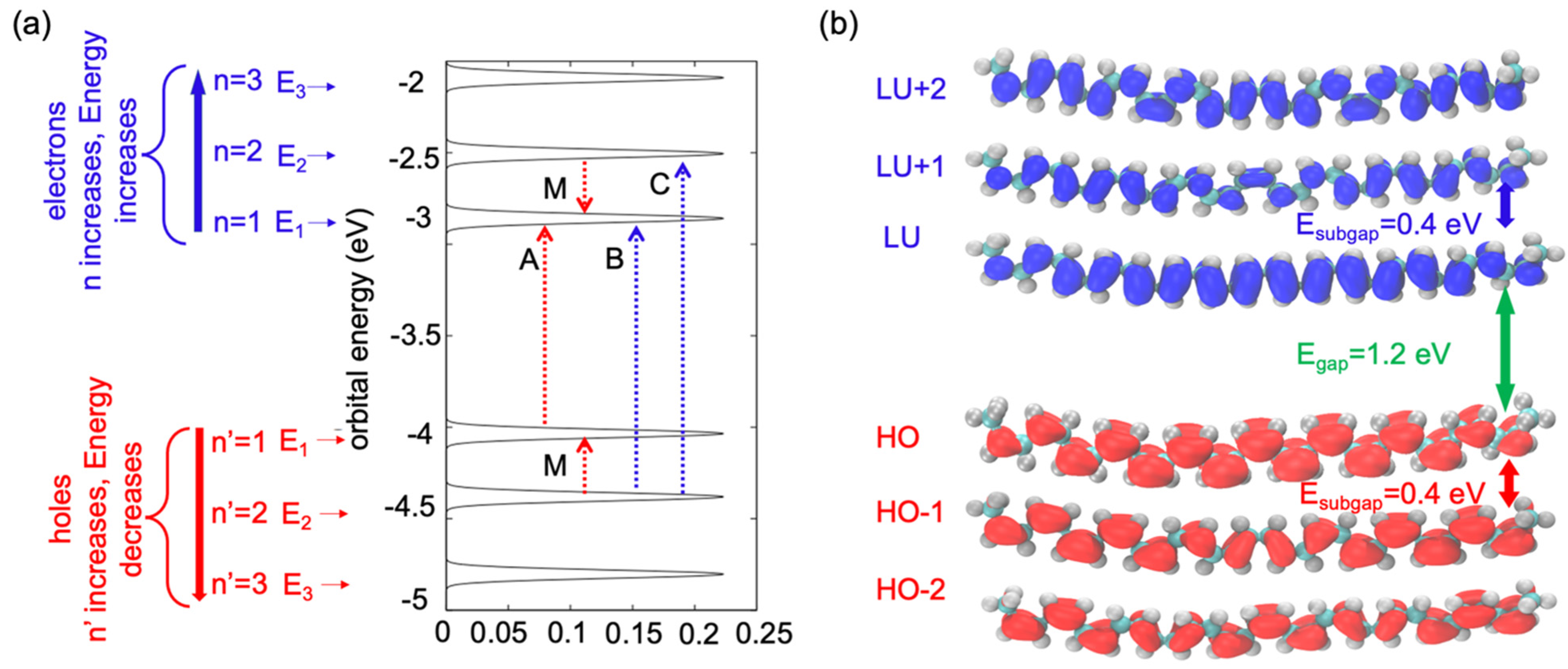
Figure 2 indicates the energy patterns of the frontier orbital. We used two labels for unoccupied and occupied orbitals: (a) each orbital was counted based on its occupation as $LU+\left(n-1\right)$ or $HO-\left(n^{\prime }-1\right)$, and (b) through an analogy with the particle in the box, we labelled the unoccupied orbitals with the index $n=1,2,3$ and the occupied orbitals with the index $n^{\prime }=1,2,3$. IN Figure 2a, the LU orbital shows that the energy is $E_{LU}=-3 \mathrm{eV}$. The energies of the unoccupied orbitals increase with an increase in the number of indexes n. When n = 2, the energy of the LU + 1 orbital is $E_{LU+1}=-2.5 \mathrm{eV}$ and the sub-gap between the LU and LU + 1 orbitals is around 0.4 eV. However, the HO orbital shows lower energy ($E_{HO}=-4 \mathrm{eV}$). It was observed that the energy gap between the HO and LU was $∆E_{gap}=1.2 \mathrm{eV}$, which was observed in the single-oligomer model. Because of the single oligomer model, there was less chance of hybridization between the electronic state of the orbital compared with a molecular crystal of multiple oligomers. Figure 2a shows that the gap between the HO and LU orbitals was more than the sub-gap between the HO and HO + 1 orbitals, and between the LU and LU-1 orbitals. Figure 2b illustrates the spatial isocontours of the frontier orbital ${\left|\phi \left(r\right)\right|}^2$ as computed by Equations (12) and (13). The maximum amount of the charge density of the LU orbital is shown in the middle portion of ${\left|\phi \left(r\right)\right|}^2$, whereas a lower amount of the charge density appears at the edge of the orbital. The same trend is observed for the HO orbital: the maximum amount of the charge density appears in the middle portion of the particle in the box and a lower amount of charge density is shown at the edge of the particle in the box. When n = 2 (the LU + 1 orbital and HO-1), the maximum amount of charge density changes from its original position. Because of the increase in the positive index of the eigenstate, the orbital was divided into two parts, and the maximum amount of the charge density was observed in the two middle portions of the orbital, and at the end of the edge and mid-point of the orbital, the charge density was almost zero.

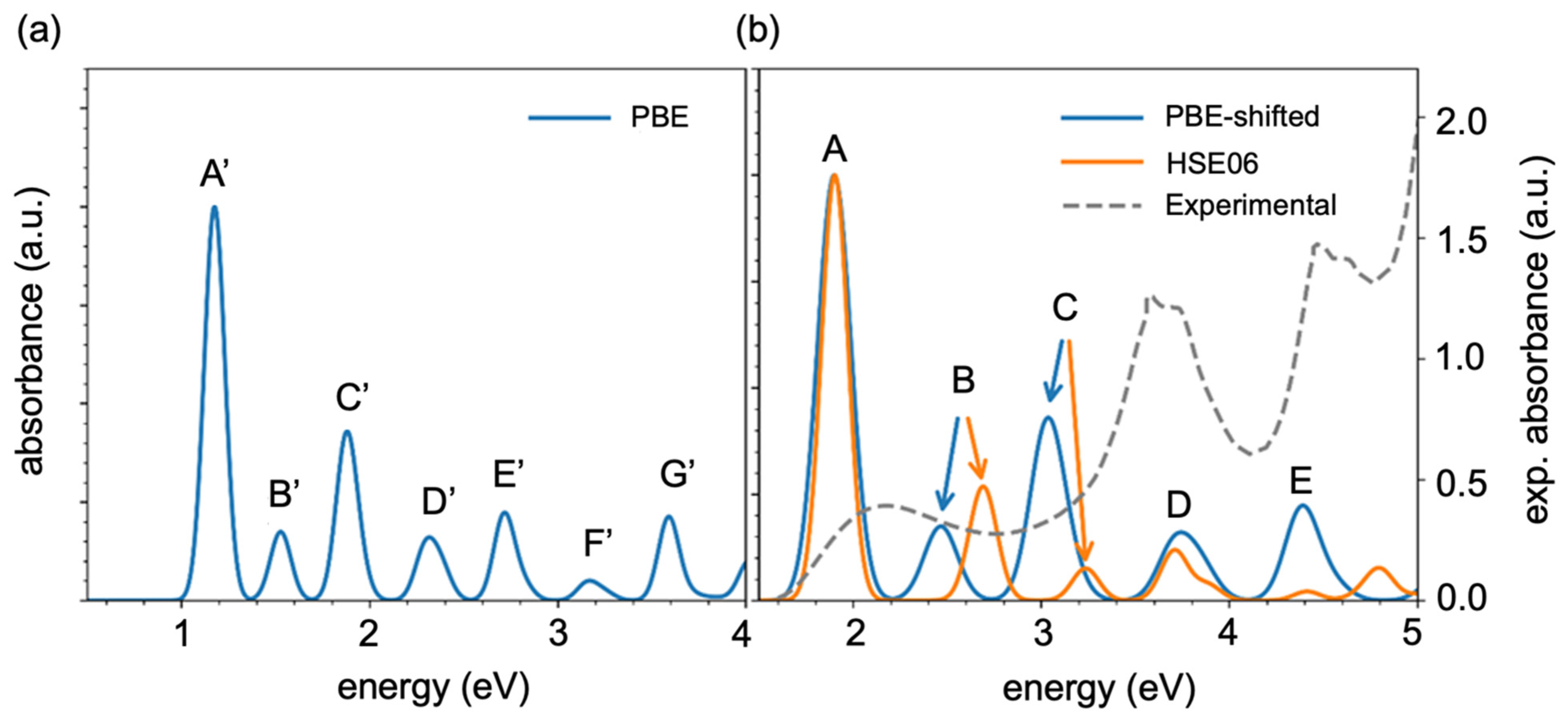
Figure 3a shows the absorption spectrum as a function of the transition energies computed by Equations (8)–(10), with intense peaks appearing from 1 eV to 4 eV. In Figure 3a,b, the peaks are labeled in the order of ascending transition energy. Here, Peak A indicates the lowest transition energy but the highest intensity of absorption, which means that bright transition occurred, whereas Peak B, Peak D, and Peak F show the highest transition energies and lower intensities of absorption, which means that they show darker transitions compared with Peaks A’, C’ and G’. To validate this using the PBE GGA function, we simulated the absorption spectra by time-dependent DFT (TDDFT) (Equation (9)) theory with an HSE06 hybrid function using Equation (5). A comparison of the TDDFT simulated and experimental absorption spectra (Table S1) indicates that the PBE GGA function underestimated the KS orbital energies, which demonstrates good qualitative agreement with the spectral features. [The comparison between the TDDFT simulated and experimental absorption spectra (Table S1) indicates that the GGA functional PBE underestimated the KS orbital energies, which shows a good qualitative agreement with the spectral features] The absorption spectra can be calculated using the PBE function shifted by a ratio (R) of the bandgap in the HSE06 and PBE function calculations, R = E_gap(HSE06)/E_gap(PBE). Figure 3b shows a comparison of the experimental spectra with the PBE simulated and HSE06 simulated absorption spectra, where the results obtained by the different functions (the PBE and HSE06 functions) qualitatively agreed with each other but there was a slight redshift in the B and C absorption peaks. Peak A shows the lowest transition energy but the highest intensity of absorption, and this occurred because of the bright transition. After we compared the simulated results with the experimental spectra, it can be concluded that the transition energies seem to agree, but the intensities and positions of peaks do not, probably because here, we looked at a single oligomer but, in the experiment, there was an ensemble.

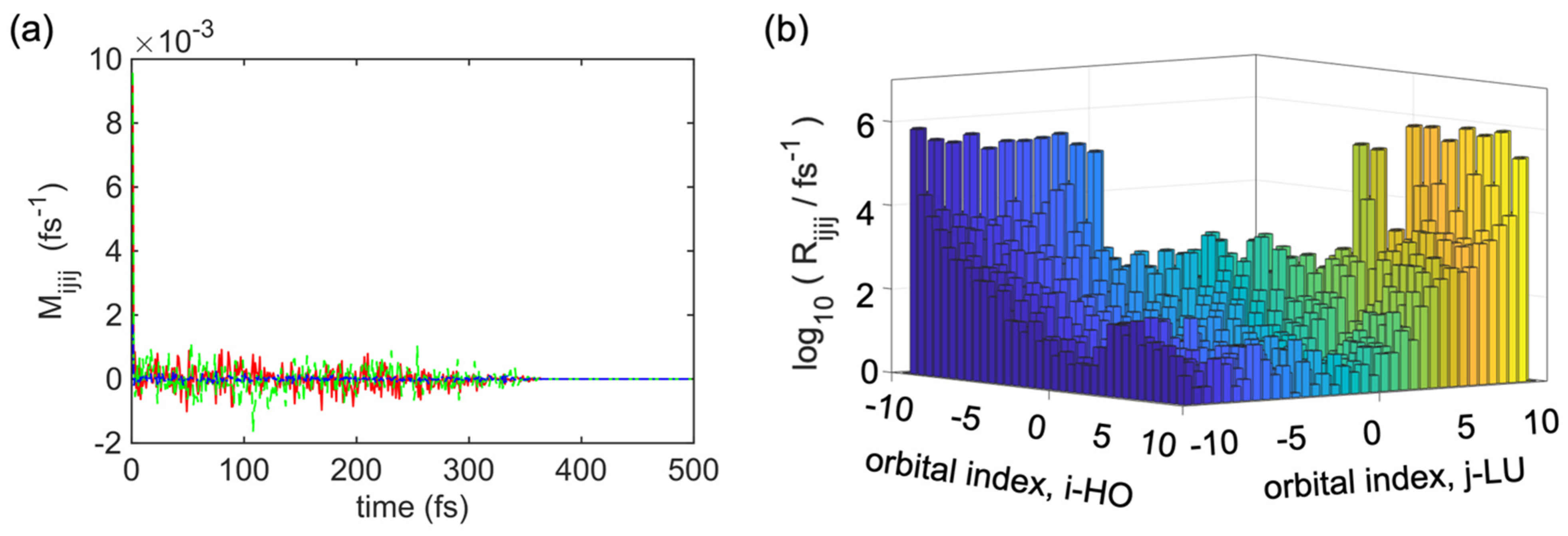
Figure 4a describes several examples of $M_{ijkl}\left(\tau \right)$. Using Equations (14)–(17), we can explain the average nonadiabatic interaction using the autocorrelation function of the electron-lattice interaction. This autocorrelation function shows several amplitudes, which provides information about the intensity of dissipative electronic transitions for the given indices $i,j,k \mathrm{and} l$. Interestingly, for any tested combination of indices, the autocorrelation function decayed abruptly within less than 5 fs, and from 0 fs to 350 fs, it showed a fluctuation in the autocorrelation function of the electron-to-lattice nonadiabatic interaction (as explained in what follows), and after 350 fs, there was no fluctuation in the autocorrelation function, as indicated by the straight line which goes up to ∞ fs. This result justifies the Markovian approximation and time-independent form of the relaxation kernel in Equations (18) and (13) [18].

At first, we extracted the Redfield tensor $R_{iijj}$ from the nonadiabatic calculations of a single oligomer of the undoped cis-polyacetylene then simulated the photoexcitation dynamics (time evolution of electron−hole pairs of orbitals) of the model. Figure 4b shows the absolute values of selected elements of $R_{iijj}$, where the blue diagonal lines refer to the valence band (VB) and the yellow diagonal lines indicate the conduction band. There are several diagonal lines from the left bottom corner to the right top corner. In the middle section, some diagonal lines are smaller than others, and the mid-section shows the lowest transition rates, which refer to nonradiative transitions, most probably occur between the nearest neighboring orbitals $\left|i-j\right|=1$. Similar results for the dominant contribution of the phonon-mediated transitions between the nearest neighboring states were obtained for $=\mathrm{CH}-{\mathrm{CH}}_3$.

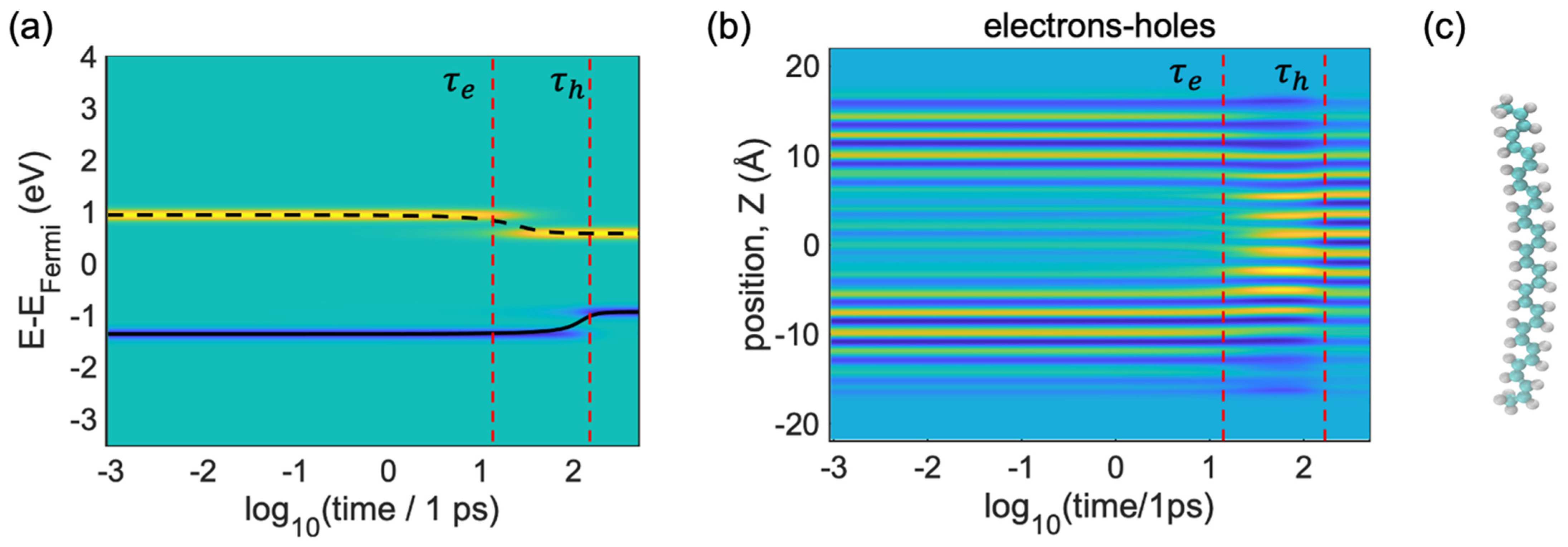
These simulation results shown in Figure 5a summarize the evolution of electron and hole states, starting from the initial photoexcitation calculated by Equation (20) with $a=\mathrm{HO}-1$, $b=\mathrm{LU}+1$. The iso-contours of the population are shown in Figure 5a, which can be $\mathsf{\Delta }n\left(a,b\right) \left(\epsilon ,t\right)$, as obtained from Equation (23), with yellow (blue) color indicating a large gain (loss) in charge density for the equilibrium distribution. In Figure 5, ${\tau }_e$ and ${\tau }_h$ define the time of relaxation/cooling for the electron and the time of relaxation/cooling for the holes. The input orbital energies and their population dynamics were provided by the ab initio electronic dynamic calculations of the model shown in Figure 5c.

Figure 5a illustrates that the nonradiative internal conversion of the photoexcited electron and hole is completed within ${10}^{1.2} \mathrm{ps}$ and ${10}^{2.5} \mathrm{ps}$, respectively. From Figure 5a we can see two spatial areas, which are highlighted by yellow and blue color. These color codes illustrate the distributions computed by Equation (23). Here, yellow areas refer to the photoexcitation of the electrons $\left(∆n>0\right)$ and the blue areas indicate the photoexcitation of the holes $\left(∆n<0\right)$. Following the yellow areas, the energy of the electron decreases from 1 eV to 0.8 eV. ${\tau }_e$ is the energy relaxation of the electron, which is visible at ${10}^{1.2} \mathrm{ps}$. After ${10}^2 \mathrm{ps}$, the energy distribution of the electron and the energy distribution of the hole is almost constant. So, from ${10}^1 \mathrm{ps}$ to ${10}^{1.2} \mathrm{ps}$, there is energy relaxation from the higher energy level (the LU + 1 orbital) to the lower energy level (the LU orbital); here, the energy of the electron is dissipated into heat. After that, the electron population arrives at the LU orbital. That is why the energy of the electrons started to convert and, after ${10}^2 \mathrm{ps}$, the energy of the electrons showed almost constant energy.

Similarly, the blue line refers to the photoexcitation of the holes. After ${10}^2 \mathrm{ps}$, the energy of the holes (valence band) jumps from −1.5 eV to −0.8 eV. The hole population goes from the lower orbital (HO-1) to the higher orbital (HO), and after ${10}^2 \mathrm{ps}$ (the time transfer of the holes = ${\tau }_e$), we can see a transition from the HO-1 orbital (−1.5 eV) to the HO orbital (−0.8 eV); after that, the energy of the holes or valence band (blue lines) shows almost constant values. Therefore, from Figure 5a, we can say that electrons relax faster than holes.

In Figure 5b, we further analyze the evolution of the nonequilibrium charge density distribution projected onto the z-direction, calculated through visualization of the KS orbitals from Equation (31). Figure 5b can be explained with the help of Figure 1. We can see that the energy of the population transfers from higher energy to lower states. The vertical line ${\tau }_e$ shows the instant of time when the maximum amount of charge density of the electrons (yellow areas) experience transfer and the vertical line ${\tau }_h$ shows the maximum amount of charge density of the holes (blue areas) experiencing transfer; one can interpret this in terms of the pattern of particles in a box for both the occupied and unoccupied orbitals. From Figure 5b, we can see the one-dimensional orbital shapes of the HO-1, HO (blue spots), LU and LU + 1 orbitals in the z-direction (yellow spots). Because of the pattern of the HO-1 and LU + 1 orbitals (Figure 1), there are no yellow lines available in the middle section and at the edge of the box (${10}^{-3} \mathrm{ps}$ to ${10}^1 \mathrm{ps}$). After ${\tau }_e={10}^1 \mathrm{ps}$, the yellow lines have already condensed in the center. Though the yellow lines (electrons) have already condensed after ${10}^1 \mathrm{ps}$, the blue areas (holes) are still at the edges. We observed that at a time between ${10}^{1.2} \mathrm{ps}$ and ${10}^2 \mathrm{ps}$, the blue line ${\tau }_e$ and yellow lines ${\tau }_h$ stay in different areas of the space. Thus, from Figure 5b, we can say that the holes relax from the edges to the center.

Concomitant to Figure 5a, this picture shows that an electron and a hole reach the LU and HO orbitals localized mainly on the $\left(-\mathrm{C}=\mathrm{C}-\right)$. Notably, the electrons’ nonradiative relaxation is faster ${\tau }_e<{\tau }_h$ compared with the holes’ relaxation, possibly because of two reasons: (i) the energy of the excited hole’s orbital stays far behind the band edge, whereas the excited electronic orbital stays at the edge of the band, and (ii) the electron−phonon couplings are stronger than hole−phonon couplings.

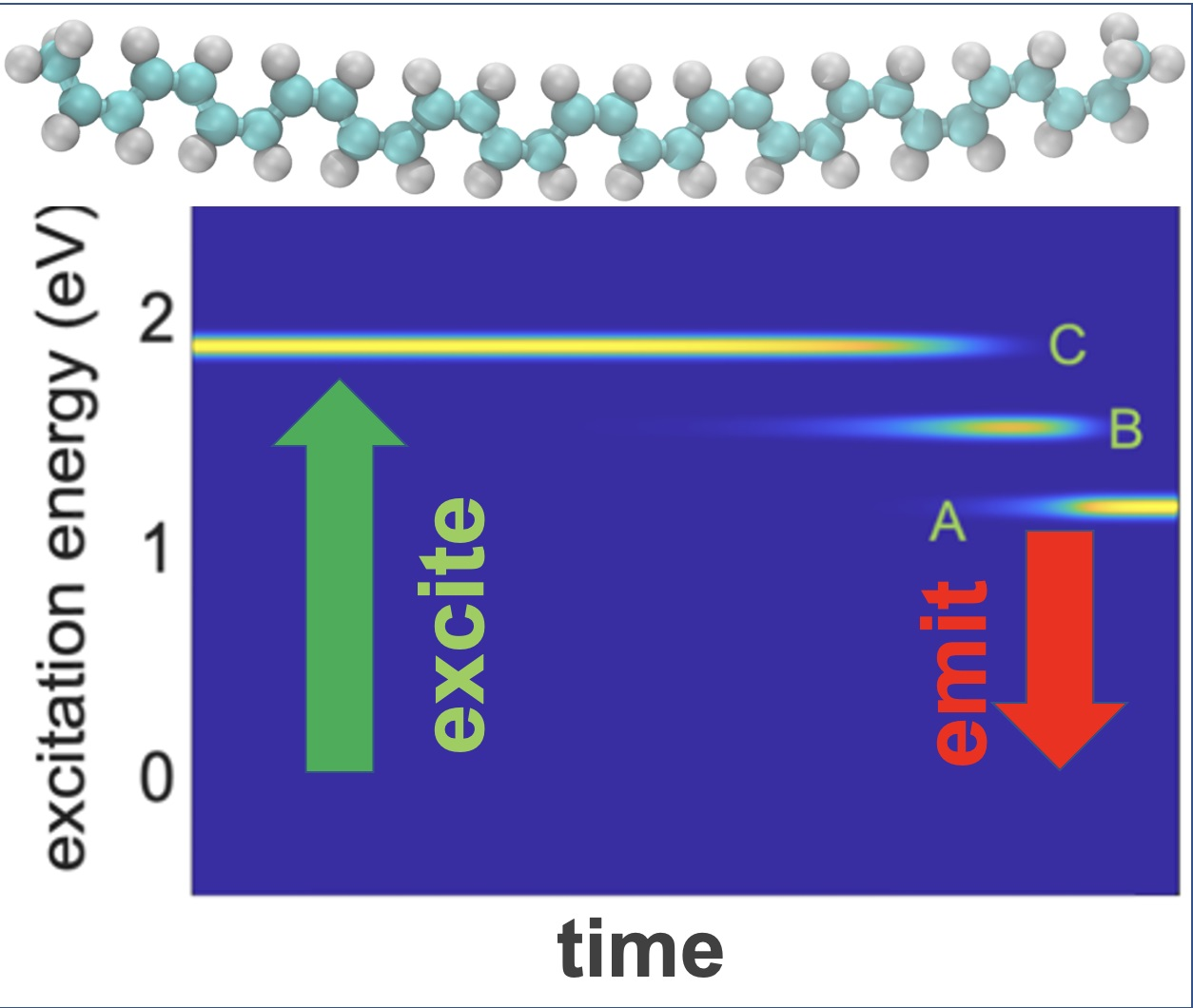
To study the dynamics of radiative and nonradiative energy dissipation in detail, we focused on photoexcitation with the energy of 2.0 eV promoting an electron from HO-1 to LU + 1, which corresponded to the D peak in the absorbance spectra. Figure 6a clearly shows the electronic energy dissipation via the lattice vibrations which occurred between about ${10}^1 \mathrm{ps}$ and ${10}^2 \mathrm{ps}$. 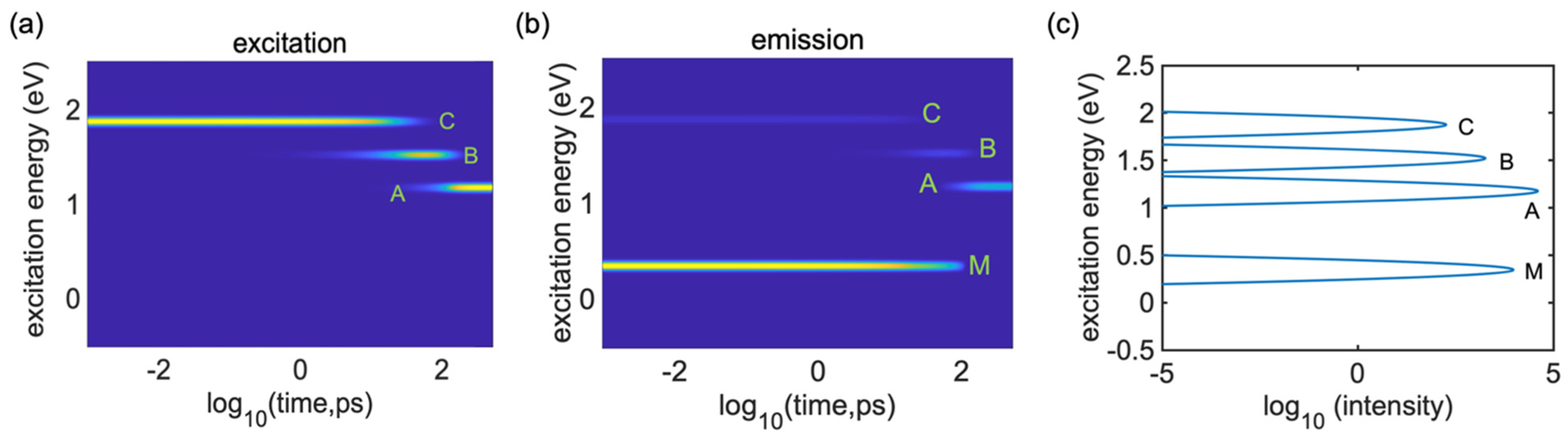Using Equation (33), we computed the time-resolved emission spectrum following the instantaneous photoexcitation at a transition energy of 2.0 eV, as displayed in Figure 6b. An emission signal in the range of 2.0 eV, which corresponds to the parent inter-band absorption from the valence band (VB) to the conduction band (CB), disappeared within 0.1 ps, reflecting the beginning of the vibrational relaxation. In Figure 6a, we can see the transition energies (Peak A, Peak B and Peak C) from 1.0 eV to 2.0 eV, which took ${10}^1 \mathrm{ps}$ to ${10}^2 \mathrm{ps}$. Peak C showed higher photoluminescence; after that, it showed weaker photoluminescence, as seen from Figure 6a (Peak B and Peak A). If we compare Figure 6a with Figure 6b, we cannot see any photoluminescence, which indicates very weak transitions. Due to the relaxation of the excitation energy, the energy started to disappear, showing the dark transition state of the system. Interestingly, there is one extra line that is visible at 0.2 eV in Figure 6b, which shows the intra-band emission features at energies below the bandgap. This also appeared in the integrated emission spectrum graph (Peak $\mathrm{M}$) but this peak is not observable in the absorption spectrum (Figure 3a) and it is noticeable in the integrated emission spectrum graph. Figure 6c presents the respective integrated emission spectrum of the single undoped cis-polyacetylene oligomer after 2.0 eV photoexcitation, which was computed by Equation (34) and demonstrates that the emission peaks are consistent with the features in Figure 6b. However, the emission features around B and C are very weak and are barely noticeable in Figure 6b, but these peaks (Peak B and Peak C) emerge in the integrated emission plot. These excitations are activated in the later stages of the dynamics (after ${10}^1 \mathrm{ps}$) and stay active for a longer period (up to ${10}^2 \mathrm{ps}$), providing a noticeable contribution to the integrated emission Peaks C at 2 eV, B at 1.5 eV and A at 1 eV.

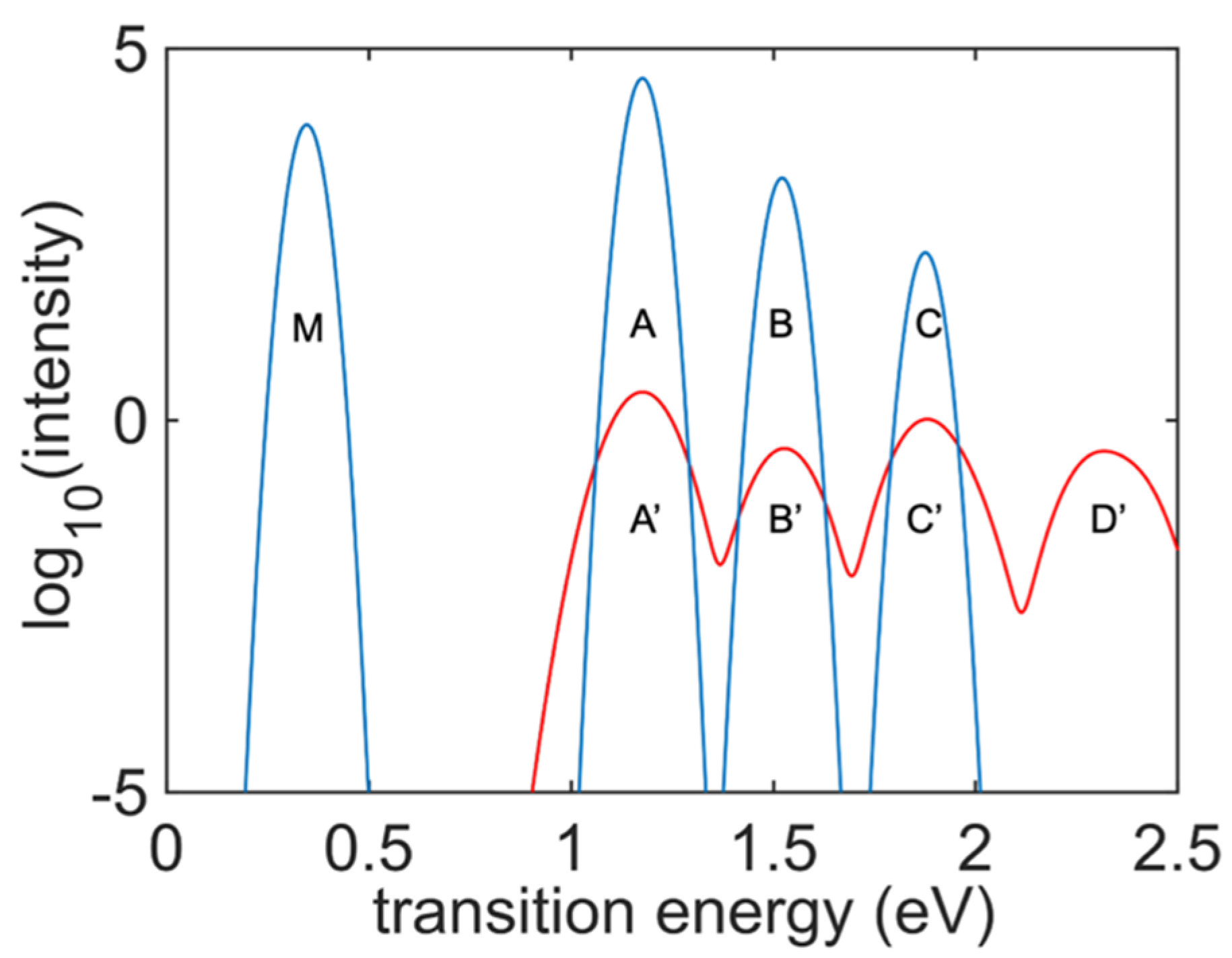
Figure 7 presents a comparison of the absorption and emission spectra of the undoped cis-polyacetylene oligomer. The absorption spectrum almost overlaps with the respective integrated emission spectrum of the model. Peak $\mathrm{A}$′ shows the lowest inter-band transition energy, which is also visible in the integrated emission spectrum. All transition energies are weaker than the other excitation energies, and one transition energy peak $\mathrm{D}$′ is absent in the integrated excitation energy graph since excitation for the PL was performed at the transition energy of Peak C. There is one additional peak (the blue Peak $\mathrm{M}$) that is visible only in the integrated emission spectrum graph but is missing in the absorption spectrum. This peak originates from transitions in the IR range, when an electron and a hole experience transitions inside the bands. Such inter-band transitions are disabled in the ground state but become available in the nonequilibrium excited state when two orbitals belonging to the same band satisfy the inverse population criterion. Computational identification of the mechanism of intra-band emission is the main finding of this work.

4. Conclusions

In this research, a model of an oligomer of a cis-polyacetylene was considered for simulating the nonadiabatic photoexcited dynamics of an undoped single cis-polyacetylene oligomer, which provides information on the nonradiative relaxation and the time-resolved photoluminescence spectra of the cis-polyacetylene polymer. Using nonadiabatic coupling, this study allows us to understand the electron dynamic properties of the system. From the nonadiabatic coupling studies, we can obtain an insight into the hole and electron dynamics of the model by monitoring what happens upon initial photoexcitation after the electrons are excited into the conduction band, leaving holes in the valence band. The absorption spectrum of the cis-polyacetylene single oligomer showed the lowest energy inter-band transitions at 1 eV. Due to lattice vibrations, the photoexcited electrons and holes relaxed to the lowest energy within ${10}^5 \mathrm{ps}$, which shows that the initial value of electronic energy relaxes towards the bandgap. It was computed that after photoexcitation, electrons relax faster than holes. Excited state dynamics are a key for understanding photoemission. Specifically, our results show similarities between the transitions shown in the absorption and emission spectra. Most of the absorption and emission spectra peaks are at the same wavelength. These peaks originate from the same pairs of orbitals. In addition, there are unique PL peaks that are not observed in the absorption. These features are the main findings of the study, attributed to intra-band transitions. Therefore, our computational model provides a detailed analysis of the optoelectronic properties of the single cis-polyacetylene oligomer, which could be used for improving nanostructured semiconductor materials for photovoltaic and LED applications.

References

1. Müllen, K.; Wegner, G. Electronic Materials: The Oligomer Approach; Wiley-VCH: Weinheim, Germany, 1998. [Google Scholar]
2. Perepichka, I.; Perepichka, D. Handbook of Thiophene-Based Materials; Wiley: Chichester, UK, 2009. [Google Scholar]
3. Han, Y.; Micha, D.; Kilin, D. Ab initio study of the photocurrent at the Au/Si metal–semiconductor nanointerface. Mol. Phys. 2014, 113, 327–335. [Google Scholar] [CrossRef]
4. Shirakawa, H.; Ito, T.; Ikeda, S. Raman Scattering and Electronic Spectra of Poly(acetylene). Polym. J. 1973, 4, 460–462. [Google Scholar] [CrossRef]
5. Poulaert, B.; Vandenhende, C.; Chielens, J.; Billaud, D.; Begin, D. Thermal conductivity of undoped trans-polyacetylene films. Solid State Commun. 1985, 55, 405–407. [Google Scholar] [CrossRef]
6. Chiang, C.; Fincher, C.; Park, Y.; Heeger, A.; Shirakawa, H.; Louis, E.; Gau, S.; MacDiarmid, A. Electrical Conductivity in Doped Polyacetylene. Phys. Rev. Lett. 1977, 39, 1098–1101. [Google Scholar] [CrossRef]
7. Carter, P.; Porter, J. Probing of π conjugation intrans-polyacetylene using near-infrared photoluminescence spectroscopy. Phys. Rev. B 1991, 43, 14478–14487. [Google Scholar] [CrossRef] [PubMed]
8. Wong, K.; Lee, C.; Tang, B. Investigation of photogenerated excited states relaxation pathways for cis rich to trans rich poly(phenylacetylene). Synth. Met. 1999, 101, 505–506. [Google Scholar] [CrossRef]
9. Yoshino, K.; Rahmat, H.; Tada, K.; Tatsuhara, S.; Kawagishi, Y.; Fujii, A.; Ozaki, M.; Teraguchi, M.; Masuda, T.; Vardeny, Z.; et al. Photoluminescence, Electroluminescence, Lasing and Novel Characteristics in Photonic Crystal, Synthetic Opal, of Conducting Polymers, Polyacetylene Derivatives. Molecular Crystals and Liquid Crystals Science and Technology. Section A. Mol. Cryst. Liq. Cryst. 1998, 322, 253–262. [Google Scholar] [CrossRef]
10. Hidayat, R.; Hirohata, M.; Tatsuhara, S.; Ozaki, M.; Teraguchi, M.; Masuda, T.; Yoshino, K. Pl and el characteristics of mixture of polyacetylene derivatives and dynamics of excitons. Synth. Met. 1999, 101, 210–211. [Google Scholar] [CrossRef]
11. Franco, I.; Rubio, A.; Brumer, P. Long-lived oscillatory incoherent electron dynamics in molecules:trans-polyacetylene oligomers. New J. Phys. 2013, 15, 043004. [Google Scholar] [CrossRef]
12. Flick, J.; Appel, H.; Rubio, A. Nonadiabatic and Time-Resolved Photoelectron Spectroscopy for Molecular Systems. J. Chem. Theory Comput. 2014, 10, 1665–1676. [Google Scholar] [CrossRef] [Green Version]
13. Moliton, A.; Hiorns, R. Review of electronic and optical properties of semiconductingπ-conjugated polymers: Applications in optoelectronics. Polym. Int. 2004, 53, 1397–1412. [Google Scholar] [CrossRef]
14. Heeger, A. Nobel Lecture: Semiconducting and metallic polymers: The fourth generation of polymeric materials. Rev. Mod. Phys. 2001, 73, 681–700. [Google Scholar] [CrossRef] [Green Version]
15. Heeger, A.; Kivelson, S.; Schrieffer, J.; Su, W. Solitons in conducting polymers. Rev. Mod. Phys. 1988, 60, 781–850. [Google Scholar] [CrossRef]
16. Tretiak, S.; Saxena, A.; Martin, R.; Bishop, A. Photoexcited breathers in conjugated polyenes: An excited-state molecular dynamics study. Proc. Natl. Acad. Sci. USA 2003, 100, 2185–2190. [Google Scholar] [CrossRef] [PubMed] [Green Version]
17. Gal, Y.-S.; Jin, S.-H.; Shim, S.-Y.; Park, J.; Son, T.-K.; Lim, K.T. Electro-optical and electrochemical properties of poly(1-ethynyl-4-phenoxybenzene). Mol. Cryst. Liq. Cryst. 2017, 659, 100–107. [Google Scholar] [CrossRef]
18. Kim, T.; Jin, S.H.; Park, J.; Lim, K.T.; Kim, S.Y.; Gal, Y.S. Polyacetylene polyelectrolyte via the non-catalyst polymerization of 2-ethynylpyridine using heptafluorobenzyl iodide. J. Ind. Eng. Chem. 2020, 87, 130–135. [Google Scholar] [CrossRef]
19. Hohenberg, P.; Kohn, W. Inhomogeneous Electron Gas. Phys. Rev. 1964, 136, B864–B871. [Google Scholar] [CrossRef] [Green Version]
20. Kresse, G.; Furthmüller, J. Efficient iterative schemes forab initiototal-energy calculations using a plane-wave basis set. Phys. Rev. B 1996, 54, 11169–11186. [Google Scholar] [CrossRef]
21. Kohn, W.; Sham, L. Self-Consistent Equations Including Exchange and Correlation Effects. Phys. Rev. 1965, 140, A1133–A1138. [Google Scholar] [CrossRef] [Green Version]
22. Moussa, J.; Schultz, P.; Chelikowsky, J. Analysis of the Heyd-Scuseria-Ernzerhof density functional parameter space. J. Chem. Phys. 2012, 136, 204117. [Google Scholar] [CrossRef] [Green Version]
23. Vydrov, O.; Heyd, J.; Krukau, A.; Scuseria, G. Importance of short-range versus long-range Hartree-Fock exchange for the performance of hybrid density functionals. J. Chem. Phys. 2006, 125, 074106. [Google Scholar] [CrossRef] [PubMed]
24. Bylander, D.; Kleinman, L. Good semiconductor band gaps with a modified local-density approximation. Phys. Rev. B 1990, 41, 7868–7871. [Google Scholar] [CrossRef] [PubMed]
25. Han, Y.; Tretiak, S.; Kilin, D. Dynamics of charge transfer at Au/Si metal-semiconductor nano-interface. Mol. Phys. 2013, 112, 474–484. [Google Scholar] [CrossRef]
26. Chen, J.; Schmitz, A.; Inerbaev, T.; Meng, Q.; Kilina, S.; Tretiak, S.; Kilin, D. First-Principles Study of p-n-Doped Silicon Quantum Dots: Charge Transfer, Energy Dissipation, and Time-Resolved Emission. J. Phys. Chem. Lett. 2013, 4, 2906–2913. [Google Scholar] [CrossRef]
27. Heyd, J.; Scuseria, G.; Ernzerhof, M. Hybrid functionals based on a screened Coulomb potential. J. Chem. Phys. 2003, 118, 8207–8215. [Google Scholar] [CrossRef] [Green Version]
28. Belletête, M.; Rivera, E.; Giasson, R.; Zhu, X.; Durocher, G. UV-Vis and fluorescence study of polyacetylenes with pendant 1-pyrenyl groups: A comparative investigation of cis- and trans-poly(1-ethynyl-pyrene). Synth. Met. 2004, 143, 37–42. [Google Scholar] [CrossRef]
Figure 1. Geometry-optimized structure (ground state) of the polymer model aligned in the y−z plane. Cyan and grey colors represent C and H atoms, respectively.
Applsci 12 02830 g001
Figure 2. Energies of the KS orbitals for single oligomer of undoped cis-polyacetylene and DOS represented by envelope functions, which follow the pattern of a particle in a box for both the occupied and unoccupied orbitals. (a) Energy of the HO, HO + 1, HO + 2, LU, LU-1 and LU-2 orbitals. Occupied/unoccupied orbitals are counted by the quantum number n’/n. A pair of such indices labels a transition. (b) The charge density of the orbitals: HO, HO + 1 and HO + 2, and LU, LU-1 and LU-2. Blue dashed lines indicate that the transition energy between the pair of orbitals in the cis-polyacetylene increased with an increase in the index of the unoccupied orbital and decreased with a decrease in the index of the occupied orbital.
Applsci 12 02830 g002
Figure 3. Experimental and calculated ground-state absorption spectra of the polyacetylene. (a) The absorption spectra were calculated using the PBE GGA function and the calculated absorption spectra using HSE06 hybrid functions [27]. (b) Energy-shifted absorption calculated using the PBE function and the experimental absorption of cis- and trans-poly(1-ethynyl-pyrene) molecules [28]. The labeling of the transitions is the same as in Figure 2.
Applsci 12 02830 g003
Figure 4. (a) Examples of autocorrelation functions for nonadiabatic coupling matrix elements, according to Equations (15) and (19). The figure shows the autocorrelation functions M i j k l ( τ ) for i = k and j = l for the following pairs of orbitals: i = HO 2 ,   j = HO 1 (green), i = HO ,   j = LU (blue) and j = LU + 1 (red). Interestingly, all of them decay abruptly within 5 fs. (b) Examples of the absolute values of Redfield tensor elements | R i i j j | used to simulate the photoexcited dynamics.
Applsci 12 02830 g004
Figure 5. (a) Iso-contours of the distribution Δ n ( a , b )   ( ε , t ) computed by Equation (23) providing the dynamics of electrons (yellow) and a hole (blue) after HO-1→LU + 1 photoexcitation in the cis-PA single oligomer; turquoise corresponds to the ground state distribution. (b) Dynamics of the spatial distribution of charge distribution Δ n ( a , b )   ( z , t ) computed by Equation (31). (c) Atomistic model of a single oligomer of cis-PA = CH CH 3 , where turquoise spheres represent carbon ( C ) and white spheres represent hydrogen ( H ) . Vertical lines labeled as τ e   and τ h   indicate the time of the population transfer between the electron and hole orbitals.
Applsci 12 02830 g005
Figure 6. Simulated photoexcited dynamics after excitation at 2.0 eV of the single undoped cis-polyacetylene oligomer. (a) Dynamics of the exciton’s (electron−hole pair) energy dissipation with time. Colors correspond to the population scale according to a continuous change in the color: yellow stands for the maximum population and navy blue for zero population. (b) Calculated time-resolved emission spectrum. Colors correspond to the intensity (oscillator strength) of the transition scaled from yellow (maximum intensity) to navy blue (zero). (c) Integrated emission spectrum, where the features A, B and C correspond to the inter-band transitions and the feature M corresponds to the intra-band transition.
Applsci 12 02830 g006
Figure 7. The transition energies and excitation energies (absorption (red) and emission/PL (blue) spectra) of the undoped single cis-polyacetylene oligomer. Note that inter-band transitions (A/A’, B/B’ and C/C’) are observed in both spectra, while the intra-band transition (M) is observed only in the PL spectrum.
Applsci 12 02830 g007
Publisher’s Note: MDPI stays neutral with regard to jurisdictional claims in published maps and institutional affiliations.