Abstract
Electrochemical machining (ECM) is a preferred advanced machining process for machining Monel 400 alloys. During the machining, the toxic nickel hydroxides in the sludge are formed. Therefore, it becomes necessary to determine the optimum ECM process parameters that minimize the nickel presence (NP) emission in the sludge while maximizing the material removal rate (MRR). In this investigation, the predominant ECM process parameters, such as the applied voltage, flow rate, and electrolyte concentration, were controlled to study their effect on the performance measures (i.e., MRR and NP). A meta-heuristic algorithm, the grey wolf optimizer (GWO), was used for the multi-objective optimization of the process parameters for ECM, and its results were compared with the moth-flame optimization (MFO) and particle swarm optimization (PSO) algorithms. It was observed from the surface, main, and interaction plots of this experimentation that all the process variables influenced the objectives significantly. The TOPSIS algorithm was employed to convert multiple objectives into a single objective used in meta-heuristic algorithms. In the convergence plot for the MRR model, the PSO algorithm converged very quickly in 10 iterations, while GWO and MFO took 14 and 64 iterations, respectively. In the case of the NP model, the PSO tool took only 6 iterations to converge, whereas MFO and GWO took 48 and 88 iterations, respectively. However, both MFO and GWO obtained the same solutions of EC = 132.014 g/L, V = 2406 V, and FR = 2.8455 L/min with the best conflicting performances (i.e., MRR = 0.242 g/min and NP = 57.7202 PPM). Hence, it is confirmed that these metaheuristic algorithms of MFO and GWO are more suitable for finding the optimum process parameters for machining Monel 400 alloys with ECM. This work explores a greater scope for the ECM process with better machining performance.
1. Introduction
For the last few decades, electrochemical machining (ECM) has been used for machining the macro- and micro-components of tool steel, carbides, superalloys, and titanium alloys. These materials are heavily used in the automotive and aerospace industries, as well as electronics, optics, medical devices, and communications. ECM is used as a high-priority machining tool because of its specific advantages, such as minor tool wear, mechanical forceless machining, no heat-affected zones, high surface quality, low roughness, and stress-free surface products. ECM is the reverse process of electroplating and can machine any hard materials or complicated shapes [1]. In ECM, the workpiece and tool are connected with the anodic pole and the cathodic pole of the electrochemical circuit, respectively, and the electrolyte is pumped through the inter-electrode gap (IEG) between the tool and the workpiece. A high-current DC power supply is allowed to pass through this electrochemical circuit to dissolve the metal from the workpiece in the form of metal hydroxides (i.e., sludge). ECM is an efficient and low-cost machining method for Ni-based alloys [2]. Several works were carried out to study the machinability of Ni alloys by ECM [3,4,5]. Ni alloys are primarily used in aircrafts, power generation turbines, rocket engines, chemical processing plants, and nuclear power plants. Poor surface traits, a short insert life, high manufacturing costs, and low productivity are associated with the machining of nickel alloys.
Monel 400 alloy is one of Ni alloys that exhibits excellent characteristics of corrosive resistance, strength, and toughness in challenging conditions [6]. When machining Ni-based alloys, ECM generates a large quantity of toxic sludge in the form of Ni and chromium hydroxides aside from gaseous byproducts, acids, sulphates, nitrates, oils, and metal ions. Environmentally sustainable machining of Ni-based alloys in ECM is needed while maintaining productivity and quality [7]. However, the discharge of nickel ions into the electrolyte slurry is significant. Therefore, it is necessary to use ECM with proper cutting conditions so that it produces sludge with fewer toxic byproducts. This hazardous emission may be retained in the electrolyte by repeated use of the electrolyte. However, such a process might decrease the machining performance. Thus, it is proposed to have optimized ECM process parameters to produce a better MRR and fewer hazardous material emissions. To the best of the authors’ knowledge, investigating the amount of nickel present in the sludge during electrochemical machining of Monel 400 alloys has not been attempted before. Optimizing the process parameters is an essential task in the ECM process, as the optimum process parameters improve the performance and economics of machining. The selection of ECM process parameters is carried out based on the experience and expertise of the machinist or machining handbooks. The process parameters selected based on the operator’s experience rarely assure high efficiency and quality machining. The machining handbooks can be a handy choice for a few applications only. In most cases, the selected optimum process parameters are far from the best, and this hampers the best utilization of ECM. Selecting the optimum values for the process parameters without proper optimization requires elaborate, costly, time-consuming, and tedious experimentation. Therefore, researchers have used different soft computing techniques to optimize the ECM process parameters in various operations [8]. Mukherjee and Chakraborty implemented a biogeography-based optimization (BBO) algorithm in ECM to determine the optimum machining conditions [9]. The BBO algorithm was inspired by the migration behavior of species among the habitats in nature. A genetic algorithm (GA) was integrated with a desirability function (DF) for simultaneous optimization of multiple objectives of the ECM process [10]. The particle swarm optimization (PSO) algorithm was adopted as an optimization strategy for determining the optimum parameters [11]. The PSO algorithm mimics the concept of the social interaction of birds in a flock. To perform the multi-objective optimization, the cuckoo optimization algorithm (COA) was used with the objective function, which was derived from the adaptive neuro-fuzzy inference system (ANFIS) model [12]. The COA was developed based on the obligate brood parasitism of some cuckoo species. A multi-objective Jaya (MO-Jaya) algorithm was implemented in the ECM process to obtain multiple optimal solutions [13]. The differential evolution (DE) algorithm has been used for both the single- and multi-objective optimization of process parameters [14]. Singh and Shukla (2017) considered the ECM process to evaluate the performance of the black hole algorithm (BHA). The performance measures of the MRR and overcut (OC) were taken to obtain the optimum machining parameters using the BHA [15]. The harmony search (HS) algorithm was combined with the DF so that an HS-DF optimizer was proposed to optimize the ECM process parameters [16]. Diyaley and Chakraborty conducted a comparative analysis with meta-heuristics such as the firefly algorithm (FA), DE algorithm, ant colony optimization (ACO) algorithm, and teaching-learning-based optimization (TLBO) algorithm for the optimization of various control parameters of an ECM process [17]. Apart from these meta-heuristics, artificial neural networks (ANNs) and fuzzy logic (FL) were also employed to model the ECM experiments and subsequent optimization process [18,19]. Several optimization algorithms have been reported in the literature, and their efficiency was tested with many benchmark functions and real-time applications. The grey wolf optimizer (GWO), a recently developed meta-heuristic, was proposed by Mirjalili et.al [20]. The GWO is inspired by the hunting behavior of the grey wolves in nature, and it ensures a better trade-off between the exploration and exploitation abilities of the algorithm. It was applied in many engineering applications, emphasizing its efficiency [21]. The significant characteristic of this algorithm is that it does not converge toward some local optima and helps store the best possible solutions obtained so far by its social hierarchy nature [22]. Kharwar and Verma implemented GWO to minimize milling performances (i.e., MRR, cutting force, and surface roughness) and proved the application potential in a manufacturing environment [23]. Omkar and Shalaka optimized the wire electrical discharge machining (WEDM) parameters with the GWO algorithm [24]. Shankar and Ankan experimented with the efficiency of the GWO algorithm for parametric optimization of the abrasive water jet machining (AWJM) process and found it to be successful [25].
A performance comparison of the response surface methodology (RSM), genetic algorithm (GA), and GWO algorithm was conducted for prediction of the surface roughness in ball-end milling of hardened steel, and GWO was found to be superior [26]. The grey relational analysis (GRA)-based GWO was implemented for milling experiments to determine the machining conditions of the spindle speed, feed rate, and depth of cut for the optimum surface roughness, cutting force, and MRR [27]. Mirjalili proposed another meta-heuristic, the moth-flame optimization (MFO) algorithm, which was inspired by the navigation method of moths in nature [28]. It gained attention for solving engineering optimization problems immediately. The improved MFO algorithm was proposed by Li et al. to maintain a balance between global and local searching [29]. A milling optimization problem was solved to emphasize its effectiveness in solving manufacturing problems [30]. The MFO algorithm was implemented to identify the optimal set of turning parameters to minimize the machinability indices. Its effectiveness was compared against the genetic algorithm (GA), grasshopper algorithm, GWO, and PSO algorithms and to be found superior to the other algorithms [31]. The optimization of the surface roughness in deep hole drilling was performed with the MFO algorithm [32]. The MFO algorithm was employed to optimize the process parameters of plasma arc cutting (PAC) of Inconel 718 superalloy [33]. Based on the literature on GWO, this algorithm is not utilized much in manufacturing optimization problems. These reviews conclude that the recently developed intelligent techniques are more advanced, and their scope of implementation in broader manufacturing applications can be explored. It is also noted that the efficiency of these new evolutionary algorithms (i.e., GWO and MFO algorithms) were not explored in the ECM process. The famous PSO algorithm is still being used to optimize machining parameters [34,35]. Hence, PSO is considered a benchmark algorithm to compare GWO and MFO algorithms in terms of convergence, computational time, and the actual Pareto optimal front.
2. Objectives
To determine the optimum ECM parameters for machining Monel 400 alloys for the maximum MRR and minimum nickel toxic emission in the electrolyte, meta-heuristics such as GWO, MFO, and PSO algorithms were employed.
3. Materials and Experimentation
The commercially available nickel-based alloy Monel 400 was used as a test specimen in this investigation. The chemical composition of the Monel 400 alloys is shown in Table 1 [36]. The machinability of Monel 400 alloy is very difficult, as it work hardens during machining. Therefore, it is a tough task to machine these alloys using conventional machining techniques.

Table 1.
Chemical composition of Monel 400 alloys.
The experiments were carried out on the eco-friendly electrochemical machining (EECM) tool. The schematic diagram of the EECM tool is shown in Figure 1. EECM comprises a power supply system, electrolyte supply system, filtering system, tool feed mechanism, work holding and position system, control panel, frame, and housing. The electrolyte (e.g., NaCl aqueous solution) is allowed to flow at the rate between 1 L/min and 10 L/min through the inter-electrode gap (IEG) of 0.1–0.6 mm. The direct current (DC) potential (11–15 V) with a current density of 20–110 A/cm2 is applied across IEG between a cathodic copper tool and an anodic workpiece. At low current densities, the MRR is low [37]. The higher current density of 110 A/cm2 was used to attain high current efficiency. According to Faraday’s laws of electrolysis, the anodic dissolution rate of workpiece depends on the electrochemical properties of the workpiece metal, the electrolyte properties, and the power supply conditions. The tool is fed against the anodic workpiece, which is firmly fixed on the vice. The machining conditions of IEG, voltage (V), and current (C) are set in the control panel. The filtration system consists of layers of bio-absorbents compartments and membrane filter. A photograph of the indigenously developed EECM is shown in Figure 2. The tool’s diameter and electrolyte exit hole were 8 mm and 2 mm, respectively. The operating conditions of EECM are summarized in Table 2.
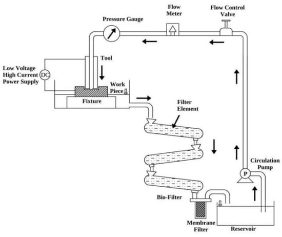
Figure 1.
Schematic diagram of EECM.
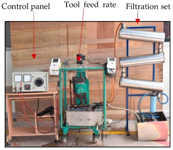
Figure 2.
EECM experimental set-up.
Table 2.
Factors and conditions of ECM experiments.
Experimental Design and Measurements
The MRR is directly proportionate to the feed rate of the tool [36]. A high feed rate leads to electrolyte boiling or choking in the tool and workpiece gap [37]. Therefore, the tool feed rate was set to the possible minimum of 0.1 mm/min to have stable movement of the tool through the workpiece. When the applied voltage is high, the current machining increases to a high MRR. A low voltage results in poor machining performance [10,11]. The voltage range of 11–16 V was considered in many such investigations in ECM to have better performance in terms of the MRR and surface finish [38,39]. Therefore, the voltage range (10–15 V) available in the set-up was used for this investigation. When the voltage is raised above a particular level, it increases the hydrogen gas bubble generation at the tool electrode, resulting in high resistivity of the electrolyte and a decrease in the current density at the workpiece [40,41,42,43]. A high concentration decreases the mobility of ions, which results in poor anodic dissolution. The concentration levels in the range of around 100–200 g/L influence the MRR significantly [10]. According to the literature, the main process parameters governing the ECM are the voltage (V), flow rate, and EC. Therefore, these parameters were considered in this investigation, and their levels are shown in Table 3.
Table 3.
Process parameters and levels.
The IEG was set to 0.1 mm, and a current of 50 A was set in the DC rectifier. The machining was performed for 5 min. The central composite design (CCD) of the response surface methodology (RSM) was adopted with the help of Minitab-17 software for the process parameters, and its levels are shown in Table 3. In this work, 20 experimental tests were carried out with different parameter combinations as shown in Figure 3. According to the concept of CCD, the center point combination was repeated 5 more times during experimentation to reduce the pure error.
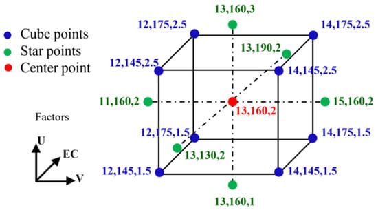
Figure 3.
Central composite design for the experimentation.
A HCl concentration of 1% was added to the NaCl electrolyte to minimize the sludge formation in the IEG. The electrolyte was pneumatically pumped from a stainless steel reservoir. A 191E water analysis kit (Environmental & Scientific Instruments Co, Haryana, India.) was used to observe the electrolyte’s pH, conductance, and temperature.
The sludge discharged from ECM was tested with atomic absorption spectroscopy (Agilent Technologies, Bangalore, India), which is shown in Figure 4. The results show the nickel content of 250 mg/L in the sludge. The precipitate of the electrolyte was tested via energy dispersive X-ray spectroscopy (EDAX, JEOL-JSM-6390, Chennai, India) and confirmed the presence of nickel. Figure 5 represents the EDAX results of the electrolyte sludge. The peaks in the figure confirm the presence of more nickel, chloride, and sodium particles. Therefore, in this invetigation, the experimental results for MRR and Nickel Presence (NP) were observed and tabulated in Table 4.
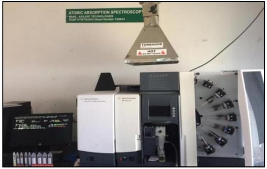
Figure 4.
Atomic absorption spectroscopy.
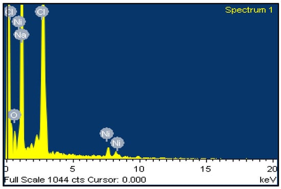
Figure 5.
EDAX spectrum for nickel in precipitate.
Table 4.
Experimental design and performance results.
4. Optimization Techniques and Procedures
The following details describe the development of mathematical models representing EECM characteristics for the MRR and the amount of nickel present, as well as the GWO and MFO techniques for optimizing the process parameters.
4.1. Mathematical Modeling of Experimentation
To study the effect of the EECM process parameters on the MRR and the discharge of nickel elements into the electrolyte, a regression model was developed to calculate the response value (as the output) in terms of different parameters (as the input). In this work, the quadratic form of the regression equation, shown in Equation (1), was established using the experimental data. The regression coefficients obtained for both the MRR and NP are shown in Table 5:
where CVij is the predicted value of the ith trial for the jth response, a, b, …, j are the coefficients of the variables, and X1, X2, and X3 are independent variables.
Table 5.
Regression coefficients for MRR and NP models.
The regression models for the given objectives can be formulated as in Equations (2) and (3):
4.2. TOPSIS Method for Multi-Objective Optimization
The Technique for Order of Preference by Similarity to Ideal Solution (TOPSIS) is a method used for converting multiple objectives into a single objective, which is consequently applied in optimization techniques for decision making [44,45]. TOPSIS is based on choosing the alternative with the shortest geometric distance from the positive ideal solution and the longest geometric distance from the negative ideal solution. By implementing the TOPSIS method, multiple objectives are converted into a single objective value. Algorithm 1 shows the the pseudo-code for TOPSIS method.
| Algorithm 1 Pseudo-code for TOPSIS. |
| 1: Read alternate and objectives matrix— with weights () and types of objectives () |
| 2: For each alternative (i = 1, 2, 3, …, m) and objective (j = 1, 2, 3, …, n) |
| 3: Compute Normalized value of using |
| 4: Calculate Performance matrix () using |
| 5: End |
| 6: For each objective (j = 1, 2, 3, …, n) |
| 7: Determine positive ideal () and negative ideal solution () |
| 8: For minimization objective— and |
| 9: For maximization objective— and |
| 10: End |
| 11: For each alternative (i = 1, 2, 3, …, m) |
| 12: Calculated Ideal and negative ideal separation () |
| 13: Determine relative closeness ( ) |
| 14: End |
| 15: Rank alternatives w.r.t. in descending order |
4.3. Grey Wolf Optimizer
The grey wolf optimizer (GWO) was inspired by the hunting behavior of grey wolves in nature. Grey wolves usually live in a pack of 5–12 members with their dominant social hierarchy [20]. The alpha (α) wolf, the pack leader, makes decisions about hunting. The beta (β) wolf helps the alpha wolf in making decisions. The omega (ω) wolves, the lowest in ranking, are responsible for submitting information to all the wolves. Others, called delta (δ) wolves, should respect alpha and beta wolves and dominate the omega wolves. The three steps in the hunting process of grey wolves are (1) tracking the prey, (2) encircling the prey, and (3) attacking the prey. GWO is simulated with the mathematical representation of the hunting process of the grey wolves to solve complex engineering problems. The optimal solution to the problem is considered the prey. To mathematically model the hunting process of these grey wolves when designing GWO, the alpha (α) wolf is considered the fittest solution. Consequently, the second- and third-best solutions are represented by beta (β) and delta (δ) wolves, respectively. The remaining candidate solutions are considered to be omega (ω) wolves.
The first step in the hunting process is encircling the prey. The mathematical formulation to mimic the encircling process for the prey and wolf are represented in the Equations (4) and (5):
where is a distance vector between the position of the prey and grey wolf. and are coefficient vectors, t is the current iteration, and and are the positions of prey and a randomly chosen grey wolf, respectively [20]. The coefficients and are determined using the following formulas:
where is a decrease from 2 to 0 linearly over the course of iterations and and are random vectors (0, 1).
A grey wolf is in the position of , updating its position according to the position of the prey . The position can be updated with respect to the current position by adjusting the values of the and vectors. This process enables the GWO to search the n-dimensional solution space of the given problem efficiently. The alpha (α), beta (β), and delta (δ) wolves guide the hunting process, and their positions are represented mathematically as in Equations (8)–(14), while the other wolves (ω) update their positions randomly:
As the value of ⃗ decreases, the search radius of the grey wolves reduces, and they get closer to the prey and attack over the last iterations of the GWO. This ensures the proper trade-off between exploration and exploitation by focusing on exploration initially and exploitation in the last iterations.
4.4. Moth-Flame Optimization Algorithm (MFO)
The moth-flame optimization (MFO) algorithm takes inspiration from the navigational mechanism (i.e., transverse orientation) of moths during night flights. The moth flies by maintaining a fixed angle relative to the moon. Since the moon is so far away from the moth, this mechanism assures the linear flight of moths. Although a lateral orientation is practical, moths are often trapped to repeatedly circle many close artificial or natural point light sources until they are exhausted. This behavior of moths is shown in Figure 6.
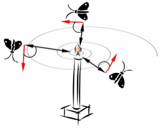
Figure 6.
Spiral flight path of moths near artificial or natural point light sources [20].
Mathematical Formulation of the MFO Algorithm
According to the MFO algorithm, the moth is considered the candidate solution to the problem. The variables are represented by the positions of the moths in the solution space. Moths can fly in the solution space by changing the position vectors. Since this algorithm is a swarm-based intelligence optimization algorithm, the position vectors of the moth population can be represented in the following matrix (Equation (15)):
where n is the number of moths and d represents the number of dimension variables to be solved. The following array represents the list of fitness value vectors corresponding to all moths:
Each moth updates its position with the corresponding unique flame to avoid the algorithm being trapped in the optimal local value, which significantly supports the algorithm’s exploration ability. Hence, the flame positions in the solution space corresponding to its moths are represented in the following array (Equation (6)):
For these flames, the corresponding column of the fitness value vectors is represented as follows:
The position update strategies for both the moth and flame matrices are different during the iteration process. The moths are the solution points that move within the solution space, and the flames are the best solution points obtained by moths iteratively so far. The best solutions of the moths are updated to the positions of the flames in the next iteration. With this approach, the MFO algorithm can find the optimal global solution. The position update behavior of each moth relative to a flame is expressed mathematically by the following equation:
where is the ith moth, is the jth flame, and S is the spiral function.
The spiral function’s initial point should start from the position of the moth, and the endpoint should be at the position of the flame. The range fluctuation of the spiral function should not exceed the boundaries of the search space. According to the above conditions, the logarithmic spiral function of the moth’s flight path is defined as in Equation (20):
where is the linear distance of the ith moth for the jth flame and b is an index of the shape of the logarithmic spiral. The magnitude of t is represented by Equation (21), where a is represented by Equation (22):
The path coefficient t ∈ [r, 1] represents the distance between the moth and the flame’s position in the next optimization iteration. The variable r decreases linearly from −1 to −2 as the number of iterations in the optimization iteration increases. The coefficient from t = −1 to −2 represents that the moths’ position is close to the flame, and t = 1 shows that the moths are farther from the flame:
Di is expressed as follows:
The above equations ensure the algorithm’s balanced global and local search capabilities. When the value of t is smaller, the moth converges to the flame. As the moth gets closer to the flame, its position around the flame is updated more quickly. After each iteration, the flames are updated based on fitness values. In the next iteration, the moth updates its position according to the updated sequence of the flame. The first moth updates its position with the flame’s best fitness value, and the last moth updates its position with the worst fitness value in the list. Hence, the flame position matrix F contains the optimal solutions of the current iteration. The number of flames can be reduced adaptively in the iterative process to balance the algorithm’s global search and local search capability in the solution space as follows:
where l is the current iteration number, N is the initial maximum number of flames, and T represents the maximum number of iterations.
5. ANOVA and Parametric Influence on Performances
Analysis of variance (ANOVA) on the process parameters and the effects of the main process parameters on the performance measures was performed. This and Fisher’s test (F-ratio) were performed to justify the adequacy of the developed regression models as in Equations (2) and (3). Values of “Prob > F” less than 0.05 indicate the model’s significance and terms. Values greater than 0.1 indicate that the model terms are insignificant.
The model F-values in Table 6 indicate that the developed models were very significant. The two-way interaction terms such as EC*V, EC*EC, and V*FR for the MRR and NP models were insignificant when the values of “Prob > F” were greater than 0.05. The terms V*V and EC*FR for the MRR and NP models, respectively, were not significant, but the coefficient of determination values for both models were good, as shown in Table 7. The normal probability curves in Figure 7 confirm the adequacy of the model equations. The high coefficient of determination values (R2 = 90.34% for the MRR and R2 = 92.29% for the NP) for both responses confirm its adequacy for optimization study.
Table 6.
Analysis of variance for quadratic models of MRR and NP.
Table 7.
Model summary.
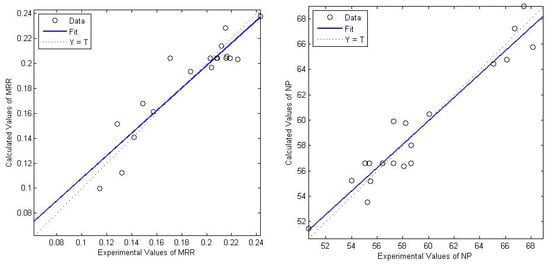
Figure 7.
Normal probability plots for MRR and NP.
Parametric Influence on the Performance Measures
Figure 8 depicts the surface plots of the MRR and NP responses for electrochemical machining of Monel 400 alloys. In each surface plot, one parameter was kept constant, and other parameters were varied with defined levels. The surface plots show that the machining parameters V, FR, and EC influenced the material removal and the discharge of nickel elements in the sludge significantly. It can be observed that the change in electrolyte concentration from 150 g/L to 190 g/L gradually increased the sludge removal. A higher concentration helped increase the speed of the electrochemical reactions and resulted in more removal (Zhang, 2010; Ayyappan and Sivakumar, 2015). A lower concentration led to a lower ion content, which reduced the rate of the electrochemical reaction (Trimmer, Hudson, Kock, and Schuster, 2003). A flow rate above 1.5 L/min removed the sludge from the gap between the tool and the workpiece better and exposed the specimen’s new surface for different electrochemical reactions (Ayyappan and Sivakumar, 2014). High flow rates increased the nickel ions in the electrolyte discharge and the MRR (Bhattacharyya and Sorkhel, 1999).
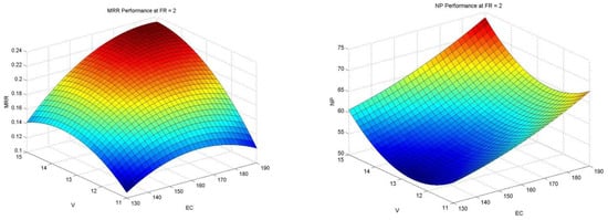
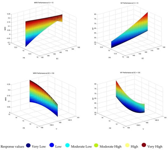
Figure 8.
Surface plot of responses for various combinations of parameters.
Figure 9 represents the main effect plots of the MRR and NP responses using MiniTab17 software. It was noticed that the electrolyte flow rate and electrolyte concentration were the influencing factors for the MRR and NP, respectively. Variations in the voltage also produced significant results in the responses.
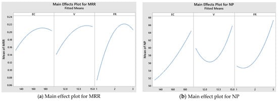
Figure 9.
Main effects plots of MRR and NP.
Figure 10 shows the interaction plots of the ECM parameters for different process attributes. As shown, the interaction terms such as EC*V and V*FR had a lean influence on the responses. The MRR and NP models were insignificant when the “Prob > F” values were more significant than 0.05. The term EC*FR influenced the NP at a high flow rate of 3 L/min.
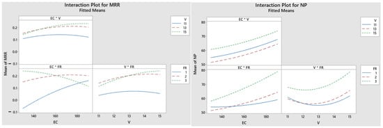
Figure 10.
Interaction plots for MRR and NP.
6. Multi-Objective Optimization of ECM Process Parameters
6.1. RSM Optimization Tool
Since the RSM as a DOE strategy was employed in this work, the optimum process parameters were obtained with its built-in optimization tool. The RSM optimization tool used the steepest ascent (SA) method combined with the desirability function (DF) for finding the optimum parameters. The variables and response constraints were set as shown in Table 8.
Table 8.
Limits of process and performance parameters.
Table 9.
Multiple response prediction results using RSM.
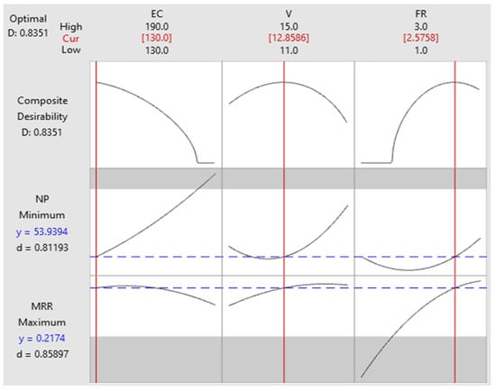
Figure 11.
Response optimization plot.
6.2. Applications of Meta-Heuristics for Optimization of the Process Parameters
To apply the various meta-heuristic algorithms such as MFO, GWO, and PSO in this work, the TOPSIS method was adopted to convert the multiple objectives into a single objective. A performance comparison of these algorithms was carried out. The Algorithms 2–4 show the pseudo-codes of the MFO, GWO, and PSO respectively.
| Algorithm 2 Grey Wolf Optimization Algorithm |
| 1: Initialize no. of grey wolf (Xij—i =1,2,..nw and j = 1,2,..nd) 2: While (it < nitr) 3: Determine the fitness function Fik 4: Calculate Pareto optimal distance fi 5: Sort fi in descending order and set as sfi 6: Store the first wolf’s data as Xit. and Fit. 7: Using the sorted data, assign Xa. = X1, Xb. = X2. and Xd. = X3. 8: Compute a = 2-it*(2/nitr) 9: For each wolf, Update the position using A1 = 2*a*rand()-a 10: C1 = 2*rand() 11: Da. = abs(C1*Xa.-X i.) 12: X1. = Xa.-A1*Da. 13: A2 = 2*a*rand()-a 14: C2 = 2*rand() 15: Db. = abs(C1*Xb.-Xi.) 16: X2. = Xb.-A2*Db. 17: A3 = 2*a*rand()-a 18: C3 = 2*rand() 19: Dd. = abs(C1*Xd.-X i.) 20: X3. = Xd.-A3*Dd. 21: X i. = (X1. + X2. + X3.)/3 22: Check Xi. within bounds 23: End 24: End 25: Using TOPSIS method convert Fit. into fi 27: Sort fi in descending order and display the first wolf’s data (optimum data) 28: Print the best solution |
| Algorithm 3 Moth-Flame Optimization Algorithm |
| 1: Initialize the parameters for Moth-flame 2: Initialize Moth position Mi randomly 3: For each i = 1:n Calculate the fitness valute fi 4: End 5: While (i ≤ imax) 6: Update the position of Mi 7: Calculate the no. of flames 8: Compute the fitness value fi 9: If (i = 1) then F = sort (M) OF = sort (OM) 10: Else F = sort (Mt-1, Mt) OF = sort (Mt-1, Mt) 11: End 12: For each i = 1:n 13: For each j = 1:d Update the values of r and t 14: Calculate the value of D w.r.t. corresponding Moth 15: Update M(i,j) w.r.t. corresponding Moth 16: End 17: End 18: End 19: Print the best solution |
| Algorithm 4 Particle Swarm Optimization Algorithm |
| 1: Initialize Particle Position P 2: For i = 1 to itrmax 3: For each particle p in P 4: Evaluate fp = f(p) 5: If fp is better than f(pB); pB= p; 6: End 7: End 8: gB= best p in P 9: For each particle p in P 10: Compute v = v + c1*rand()*(pB– p) + c2 *rand()*(gB-p) 11: Update p = p + v 12: End 13: End 14: Print the best solution |
The terms in GWO and their equivalent meanings in the optimization problem are listed in Table 10.
Table 10.
Terms in GWO and optimization problems.
Similarly, the equivalent terms for the MFO and PSO algorithms for an optimization problem are shown in Table 11. The algorithm parameters are shown in Table 12.
Table 11.
Terms in MFO and PSO optimization problems.
Table 12.
Algorithm parameters for GWO, MFO, and PSO algorithms.
The steps in implementing the GWO algorithm in this experimentation are shown in Figure 12. The flowchart for implementing the MFO algorithm in the present work is shown in Figure 13.
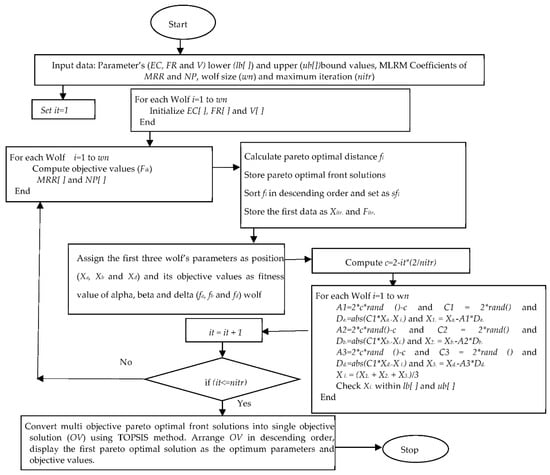
Figure 12.
Implementation of GWO algorithm.
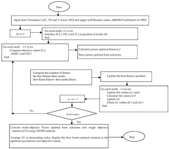
Figure 13.
Implementation of MFO algorithm.
The PSO implementation is shown in Figure 14. The efficiency of these algorithms is compared in the convergence plot of Figure 15. In maximization of the MRR, the MFO convergence plot was attained after the 60th iteration, while GWO and PSO performed better. In minimization of the NP, PSO converged well before MFO and GWO.
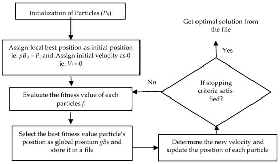
Figure 14.
Implementation of PSO algorithm.
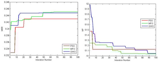
Figure 15.
Comparison of convergence plots for various algorithms for MRR and NP.
The optimum process parameters obtained by different meta-heuristics and the RSM are tabulated in Table 13. The convergence plot of the Pareto optimal solutions is shown in Figure 16, and the Pareto optimal set of process parameters out of 12 runs is presented in Table 14.
Table 13.
Optimum process parameters and the response values.
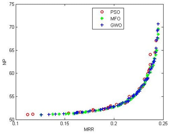
Figure 16.
Pareto optimal solutions for various algorithms.
Table 14.
The Pareto optimal solutions and their responses for various algorithms.
Both the MFO and GWO algorithms produced the better trade-off performances with the same solutions of EC = 132.014 g/L, V = 13. 2406 V, and FR = 2.8455 L/min for MRR = 0.242 g/min and NP = 57.7202 PPM.
7. Conclusions
In the present study, ECM operations were carried out on Monel 400 alloys by varying the applied voltage (11–15 V), flow rate (1–3 L/min), and electrolyte concentration (130–190 g/L). The meta-heuristic algorithms (i.e., moth-flame optimization (MFO) algorithm, grey wolf optimizer (GWO), and particle swarm optimization (PSO)) were implemented to find out the optimum process parameters for producing the best performance measures for the material removal rate (MRR) and nickel presence (NP) in the sludge. The regression model equations were developed to determine the optimum parametric combination. The high coefficient of determination values (R2 = 90.34% for MRR and R2 = 92.29% for NP) for both responses confirmed their adequacy. The algorithms were tuned to obtain the best possible feasible solution. This study proved that the MFO and GWO algorithms could be successfully utilized to find the best process parameter setting for the ECM process for Monel 400 alloys. The TOPSIS algorithm was implemented to convert multiple objectives into a single objective used in meta-heuristic algorithms. It was observed from the surface, main, and interaction plots of this ECM experimentation that all the process variables significantly affected the performances. The PSO algorithm converged very quickly in 10 iterations, while GWO and MFO took 14 and 64 iterations, respectively, for convergence of the MRR. In the case of the NP model, the PSO tool took only six iterations to converge, whereas MFO and GWO took 48 and 88 iterations, respectively. However, both MFO and GWO obtained the better trade-off performances with the same solutions of EC = 132.014 g/L, V = 13. 2406 V, and FR = 2.8455 L/min for MRR = 0.242 g/min and NP = 57.7202 PPM. The Pareto optimal set of solutions provided by the GWO, MFO, and PSO algorithms for the ECM process was beneficial to the industries, as it contained a wide range of optimal values. A particular solution from the Pareto optimal set can be chosen according to the specific needs of the objectives. Hence, it was confirmed that the metaheuristic algorithms of MFO and GWO were suitable for finding the optimum process parameters for machining Monel 400 alloys with ECM. Future studies may be explored by combining the artificial neural network (ANN) and fuzzy logic (FL) concepts with MFO and GWO to determine the optimum ECM process parameters.
Author Contributions
Conceptualization and methodology, V.N., A.S., L.N. and S.K.M.; writing—original draft preparation, V.N., A.S., L.N. and S.K.M.; writing—review and editing, S.S., E.A.N., R.S. and H.M.A.M.H. All authors have read and agreed to the published version of the manuscript.
Funding
The authors extend their appreciation to King Saud University for funding this work through Researchers Supporting Project number (RSP-2021/164), King Saud University, Riyadh, Saudi Arabia.
Institutional Review Board Statement
Not applicable.
Informed Consent Statement
Not applicable.
Data Availability Statement
Not applicable.
Conflicts of Interest
The authors declare no conflict of interest.
References
- Skoczypiec, S.; Lipiec, P.; Bizoń, W.; Wyszyński, D. Selected Aspects of Electrochemical Micromachining Technology Development. Materials 2021, 14, 2248. [Google Scholar] [CrossRef] [PubMed]
- Ge, Y.; Zhu, Z.; Wang, D. Electrochemical Dissolution Behavior of the Nickel-Based Cast Superalloy K423A in NaNO3 Solution. Electrochim. Acta 2017, 253, 379–389. [Google Scholar] [CrossRef]
- Zhang, Y.; Xu, Z.; Xing, J.; Zhu, D. Effect of tube-electrode inner diameter on electrochemical discharge machining of nickel-based super alloy. Chin. J. Aeronaut. 2016, 29, 1103–1110. [Google Scholar] [CrossRef] [Green Version]
- Ge, Y.; Zhu, Z.; Zhu, Y. Electrochemical deep grinding of cast nickel-base superalloys. J. Manuf. Process. 2019, 47, 291–296. [Google Scholar] [CrossRef]
- Bi, X.; Zeng, Y.; Qu, N. Wire electrochemical micromachining of high-quality pure-nickel microstructures focusing on different machining indicators. Precis. Eng. 2020, 61, 14–22. [Google Scholar] [CrossRef]
- Tayal, A.; Kalsi, N.S.; Gupta, M.K.; Garcia-Collado, A.; Sarikaya, M. Reliability and economic analysis in sustainable machining of Monel 400 alloy. Proc. Inst. Mech. Eng. Part C J. Mech. Eng. Sci. 2021, 235, 5450–5466. [Google Scholar] [CrossRef]
- Rajurkar, K.P.; Hadidi, H.; Pariti, J.; Reddy, G.C. Review of Sustainability Issues in Non-Traditional Machining Processes. Procedia Manuf. 2017, 7, 714–720. [Google Scholar] [CrossRef]
- Chakraborty, S.; Bhattacharyya, B.; Diyaley, S. Applications of optimization techniques for parametric analysis of non-traditional machining processes: A Review. Manag. Sci. Lett. 2019, 9, 467–494. [Google Scholar] [CrossRef]
- Mukherjee, R.; Chakraborty, S. Selection of the optimal electrochemical machining process parameters using biogeography-based optimization algorithm. Int. J. Adv. Manuf. Technol. 2013, 64, 781–791. [Google Scholar] [CrossRef]
- Ayyappan, S.; Sivakumar, K. Investigation of electrochemical machining characteristics of 20MnCr5 alloy steel using potassium dichromate mixed aqueous NaCl electrolyte and optimization of process parameters. Proc. Inst. Mech. Eng. Part B J. Eng. Manuf. 2015, 229, 1984–1996. [Google Scholar] [CrossRef]
- Ayyappan, S.; Sivakumar, K. Enhancing the performance of electrochemical machining of 20MnCr5 alloy steel and optimization of process parameters by PSO-DF optimizer. Int. J. Adv. Manuf. Technol. 2016, 82, 2053–2064. [Google Scholar] [CrossRef]
- Sohrabpoor, H.; Khanghah, S.; Shahraki, S.; Teimouri, R. Multi-objective optimization of electrochemical machining process. Int. J. Adv. Manuf. Technol. 2016, 82, 1683–1692. [Google Scholar] [CrossRef]
- Rao, R.V.; Rai, D.P.; Balic, J. A multi-objective algorithm for optimization of modern machining processes. Eng. Appl. Artif. Intell. 2017, 61, 103–125. [Google Scholar] [CrossRef]
- Mehrvar, A.; Basti, A.; Jamali, A. Inverse modelling of electrochemical machining process using a novel combination of soft computing methods. Proc. Inst. Mech. Eng. Part C J. Mech. Eng. Sci. 2020, 234, 3436–3446. [Google Scholar] [CrossRef]
- Singh, D.; Shukla, R. Parameter optimization of electrochemical machining process using black hole algorithm. IOP Conf. Ser. Mater. Sci. Eng. 2017, 282, 012006. [Google Scholar] [CrossRef] [Green Version]
- Kalaimathi, M.; Venkatachalam, G.; Sivakumar, M.; Ayyappan, S. Multi-response optimisation of electrochemical machining process parameters by harmony search-desirability function optimiser. Int. J. Manuf. Technol. Manag. 2020, 34, 331–348. [Google Scholar] [CrossRef]
- Diyaley, S.; Chakraborty, S. Optimization of electrochemical machining process parameters using teaching-learning-based algorithm. AIP Conf. Proc. 2020, 2273, 050010. [Google Scholar] [CrossRef]
- Kasdekar, D.K.; Parashar, V.; Arya, C. Artificial neural network models for the prediction of MRR in Electro-chemical machining. Mater. Today Proc. 2018, 5 Pt 1, 772–779. [Google Scholar] [CrossRef]
- Chakraborty, S.; Das, P.P.; Kumar, V. Application of grey-fuzzy logic technique for parametric optimization of non-traditional machining processes. Grey Syst. Theory Appl. 2018, 8, 46–68. [Google Scholar] [CrossRef]
- Mirjalili, S.; Mirjalili, S.M.; Lewis, A. Grey Wolf Optimizer. Adv. Eng. Softw. 2014, 69, 46–61. [Google Scholar] [CrossRef] [Green Version]
- Li, Y.; Lin, X.; Liu, J. An Improved Gray Wolf Optimization Algorithm to Solve Engineering Problems. Sustainability 2021, 13, 3208. [Google Scholar] [CrossRef]
- Khalilpourazari, S.; Khalilpourazary, S. Optimization of production time in the multi-pass milling process via a robust grey wolf optimizer. Neural Comput. Appl. 2018, 29, 1321–1336. [Google Scholar] [CrossRef]
- Kharwar, P.K.; Verma, R.K. Nature instigated Grey wolf algorithm for parametric optimization during machining (Milling) of polymer nanocomposites. J. Thermoplast. Compos. Mater. 2021, 1–23. [Google Scholar] [CrossRef]
- Kulkarni, O.; Kulkarn, S. Process Parameter Optimization in WEDM by Grey Wolf Optimizer. Mater. Today Proc. 2018, 5 Pt 1, 4402–4412. [Google Scholar] [CrossRef]
- Chakraborty, S.; Mitra, A. Parametric optimization of abrasive water-jet machining processes using grey wolf optimizer. Mater. Manuf. Process. 2018, 33, 1471–1482. [Google Scholar] [CrossRef]
- Sekulic, M.; Pejic, V.; Brezocnik, M.; Gostimirović, M.; Hadzistevic, M. Prediction of surface roughness in the ball-end milling process using response surface methodology, genetic algorithms, and grey wolf optimizer algorithm. Adv. Prod. Eng. Manag. 2018, 13, 18–30. [Google Scholar] [CrossRef]
- Kharwar, P.K.; Verma, R.K. Exploration of nature inspired Grey wolf algorithm and Grey theory in machining of multiwall carbon nanotube/polymer nanocomposites. Eng. Comput. 2020, 1–22. [Google Scholar] [CrossRef]
- Mirjalili, S. Moth-Flame Optimization Algorithm: A Novel Nature-inspired Heuristic Paradigm. Knowl.-Based Syst. 2015, 89, 228–249. [Google Scholar] [CrossRef]
- Li, Y.; Zhu, X.; Liu, J. An Improved Moth-Flame Optimization Algorithm for Engineering Problems. Symmetry 2020, 12, 1234. [Google Scholar] [CrossRef]
- Yıldız, B.; Yildiz, A.R. Moth-flame optimization algorithm to determine optimal machining parameters in manufacturing processes. Mater. Test. 2017, 59, 425–429. [Google Scholar] [CrossRef]
- Sivalingam, V.; Sun, J.; Mahalingam, S.K.; Nagarajan, L.; Natarajan, Y.; Salunkhe, S.; Nasr, E.A.; Davim, J.P.; Hussein, H.M.A.M. Optimization of Process Parameters for Turning Hastelloy X under Different Machining Environments Using Evolutionary Algorithms: A Comparative Study. Appl. Sci. 2021, 11, 9725. [Google Scholar] [CrossRef]
- Kamaruzaman, A.F.; Mohd Zain, A.; Alwee, R.; Md Yusof, N.; Najarian, F. Optimization of Surface Roughness in Deep Hole Drilling using Moth-Flame Optimization. ELEKTRIKA-J. Electr. Eng. 2019, 18, 62–68. [Google Scholar] [CrossRef]
- Karthick, M.; Anand, P.; Siva Kumar, M.; Meikandan, M. Exploration of MFOA in PAC parameters on machining Inconel 718. Mater. Manuf. Process. 2021, 1–13. [Google Scholar] [CrossRef]
- Lmalghan, R.; Rao, M.C.K.; Arunkumar, S.; Rao, S.S.; Herbert, M.A. Machining Parameters Optimization of AA6061 Using Response Surface Methodology and Particle Swarm Optimization. Int. J. Precis. Eng. Manuf. 2018, 19, 695–704. [Google Scholar] [CrossRef]
- Abu-Mahfouz, I.; Banerjee, A.; Rahman, E. Evolutionary Optimization of Machining Parameters Based on Surface Roughness in End Milling of Hot Rolled Steel. Materials 2021, 14, 5494. [Google Scholar] [CrossRef]
- Kalaimathi, M.; Venkatachalam, G.; Sivakumar, M.; Ayyappan, S. Experimental investigation on the suitability of ozonated electrolyte in travelling-wire electrochemical machining. J. Braz. Soc. Mech. Sci. Eng. 2017, 39, 4589–4599. [Google Scholar] [CrossRef]
- Ayyappan, S.; Sivakumar, K. Experimental investigation on the performance improvement of electrochemical machining process using oxygen-enriched electrolyte. Int. J. Adv. Manuf. Technol. 2014, 75, 479–487. [Google Scholar] [CrossRef]
- Qu, N.; Fang, X.; Li, W.; Zeng, Y.; Zhu, D. Wire electrochemical machining with axial electrolyte fushing for titanium alloy. Chin. J. Aeronaut. 2013, 26, 224–229. [Google Scholar] [CrossRef] [Green Version]
- Qu, N.S.; Ji, H.J.; Zeng, Y.B. Wire electrochemical machining using reciprocated traveling wire. Int. J. Adv. Manuf. Technol. 2014, 72, 677–683. [Google Scholar] [CrossRef]
- Leese, R.; Ivanov, A. Electrochemical micromachining: Review of factors affecting the process applicability in micro-manufacturing. Proc. Inst. Mech. Eng. Part B J. Eng. Manuf. 2018, 232, 195–207. [Google Scholar] [CrossRef]
- Zhang, Y. Investigation into Current Efficiency for Pulse Electrochemical Machining of Nickel Alloy. University of Nebraska–Lincoln. 2010. Available online: http://digitalcommons.unl.edu/imsediss/2 (accessed on 10 November 2021).
- Trimmer, A.L.; Hudson, J.L.; Kock, M.; Schuster, R. Single-step electrochemical machining of complex nanostructures with ultrashort voltage pulses. Appl. Phys. Lett. 2003, 82, 3327–3329. [Google Scholar] [CrossRef]
- Rathod, V.; Doloi, B.; Bhattacharyya, B. Experimental investigations into machining accuracy and surface roughness of microgrooves fabricated by electrochemical micromachining. Proc. Inst. Mech. Eng. Part B J. Eng. Manuf. 2015, 229, 1781–1802. [Google Scholar] [CrossRef]
- Shunmugesh, K.; Panneerselvam, K. Optimization of machining process parameters in drilling of CFRP using multi-objective Taguchi technique, TOPSIS and RSA techniques. Polym. Polym. Compos. 2017, 25, 185–192. [Google Scholar] [CrossRef]
- Balaji, K.; Siva Kumar, M.; Yuvaraj, N. Multi objective taguchi–grey relational analysis and krill herd algorithm approaches to investigate the parametric optimization in abrasive water jet drilling of stainless steel. Appl. Soft Comput. J. 2021, 102, 107075. [Google Scholar] [CrossRef]
Publisher’s Note: MDPI stays neutral with regard to jurisdictional claims in published maps and institutional affiliations. |
© 2022 by the authors. Licensee MDPI, Basel, Switzerland. This article is an open access article distributed under the terms and conditions of the Creative Commons Attribution (CC BY) license (https://creativecommons.org/licenses/by/4.0/).