Recursive Optimal Finite Impulse Response Filter and Its Application to Adaptive Estimation

Abstract

In this paper, the recursive form of an optimal finite impulse response filter is proposed for discrete time-varying state-space models. The recursive form of the finite impulse response filter is derived by employing finite horizon Kalman filtering with optimally estimated initial conditions. The horizon initial state and its error covariance on the horizon are optimally estimated by using recent finite measurements, in the sense of maximum likelihood estimation, then initiating the finite horizon Kalman filter. The optimality and unbiasedness of the proposed filter are proved by comparison with the conventional optimal finite impulse response filter in batch form. Moreover, an adaptive FIR filter is also proposed by applying the adaptive estimation scheme to the proposed recursive optimal FIR filter as its application. To evaluate the performance of the proposed algorithms, a computer simulation is performed to compare the conventional Kalman filter and adaptive Kalman filters for the gas turbine aircraft engine model.

1. Introduction

The Kalman filter has been used as a standard tool to deal with state estimation of linear state-space models. However, since the Kalman filter has infinite impulse response (IIR) structure, which makes use of whole measurements from the initial time to the current, model uncertainties which come from the limited knowledge of the system model and the statistics of the noises and computation errors may accumulate in the estimated state. These could originate the divergence problem in the Kalman filter [1,2,3]. In order to prevent divergence problems, finite impulse response (FIR) filters have been used as an alternative to the Kalman filter [4,5,6,7,8,9,10,11,12,13,14,15,16,17,18,19,20]. Since FIR filters estimate the states by using finite measurements on the most recent time interval, these filters are known to be more robust against modeling uncertainties and numerical errors that cause of divergence problem in Kalman filter. Moreover, due to their FIR structure, FIR filters have good properties such as built-in bounded input/bounded output (BIBO) stability and fast tracking speed.

However, despite the aforementioned advantages of FIR filters, their complicated derivation and batch form might lead to computational inefficiency and limitations in further developments. Since the Kalman filter is well-known and has recursive form, which can give effective computation methods to the FIR filter, the recursive form of FIR filters were introduced by modifying the Kalman filter [7,8,9,10,11,12,13,14,15,16]. In [7,8], the receding horizon Kalman (RHK) filters, whose concept is introduced in Figure 1a, and its fast iteration method, are proposed for time-invariant systems. The filter equations of RHK filters are easy to understand and many useful Kalman filtering methods could be directly applied to FIR filtering problems for improving the performance of FIR filters because they are derived by combining the Kalman filter algorithm and receding horizon strategy. Since RHK filters have exactly the same structure as the Kalman filter on the finite estimation horizon, the RHK filtering problem can be thought as a recursive finite horizon Kalman filtering problem with special initial conditions. Thus, the initial state and its error covariance for RHK filters are very important factors for the performance of estimation. However, RHK filters were derived with heuristic assumptions on initial conditions such as the infinite initial error covariance. In the derivation of the RHK filter, inversion of the state transition matrix is used in the iterative calculation to estimate state and error covariance matrix. For an infinite covariance, the inverse matrix becomes singular and the estimation problem may not be feasible. Furthermore, the optimality of RHK filters is not clear in their derivations, and they cannot be applied to time-varying systems. On the other hand, Kalman-like unbiased FIR (KUFIR) filters, whose concept is introduced in Figure 1b, are also proposed for the recursive FIR filtering [9,10,11,12,13,14,15,16]. KUFIR filtering is a recursive Kalman-like algorithm that ignores the noise statistics and initial conditions. These are ignored by determining the optimal horizon length which minimize the mean-square estimation error, then the recursive prediction and correction procedure are repeated without using noise statistics. Since the optimal horizon length is the only design parameter of the KUFIR filter, the determination of optimal horizon length is a major problem, hence, several algorithms have been developed to find the optimal horizon length. In [9], the optimal horizon length was derived for the l-degree polynomial model by minimizing the mean-square estimation error. In [11], it was measured using the correlation method, and in [12], it was determined by using a bank of KUFIR filters operating in parallel. For fast computation of the optimal horizon length, an adaptive KUFIR filter was also suggested for time-invariant systems in [15]. However, even though the horizon initial state can be ignored, the state at time $k-N_{opt}+K$ in Figure 1b considered as an actual initial state is required at each estimation horizon, and they are obtained by calculating the batch form of the filter equation. In addition to the aforementioned computational inefficiency, these approaches have a common disadvantage due to the fact that heavy computational load is also required to specify the optimal horizon length, because it must be obtained for each horizon in time-varying systems. Moreover, the optimality of KUFIR filters is not guaranteed and the horizon length cannot be adjusted.

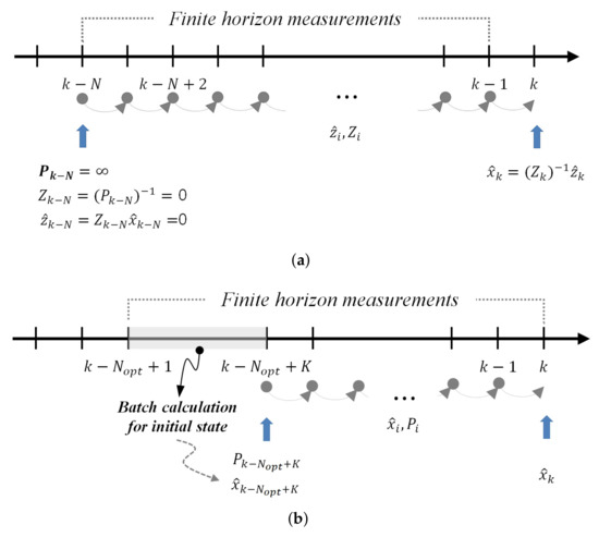
Figure 1. (a) The concept of RHK filter. (b) The concept of KUFIR filter.

Therefore, in this paper, a new recursive optimal FIR (ROFIR) filter is proposed for linear time-varying systems in order to overcome the disadvantages of previous methods for recursive FIR filtering. The ROFIR filter is derived by employing the finite horizon Kalman filter and the optimal and unbiased initial state estimation. The initial state and its corresponding error covariance on the estimation horizon are obtained by solving the maximum likelihood estimation problem, then they initiate the finite horizon Kalman filter. Since the initial state is estimated from the measurements at each finite estimation horizon, the ROFIR filter does not require any priori initial information. In addition, the proposed ROFIR filter is derived without assumption on a nonsingular state-transition matrix and has less computational burden than the KUFIR filters for time-varying systems. Furthermore, the ROFIR filter provides the best linear unbiased estimate (BLUE) of the state on the finite estimation horizon. In addition, since AFIR filters in previous studies were designed in batch form, they were mostly focused on how to adjust the horizon length [17,18,19]. To the author’s best knowledge, there are no results on the adaptive FIR (AFIR) filters which consider noise statistics, thus, we propose a new adaptive FIR filtering algorithm by employing a sequential noise statistics estimation technique as an application of the proposed ROFIR filter.

This paper is organized as follows: In Section 2, the ROFIR filter is proposed for linear time-varying state-space models and its optimality and unbiasedness are proved. Moreover, the AFIR filter is also proposed by applying the modified sequential noise statistics estimation method to the proposed ROFIR filter. In Section 3, the performance and effectiveness of the proposed ROFIR and AFIR filters are shown and discussed via computer simulations. Finally, our conclusions are presented in Section 4.

2. Recursive Optimal FIR Filter and Adaptive FIR Filter

2.1. Recursive Optimal FIR Filter with Optimally Estimated Initial Conditions

Consider the following discrete time-varying state-space model:

$$\begin{array}{ccc}\hfill x_{k+1}& =& A_k{x}_k+w_k,\hfill \end{array}$$

(1)

$$\begin{array}{ccc}\hfill y_k& =& C_k{x}_k+v_k,\hfill \end{array}$$

(2)

where $x_k$ is the state vector, $y_k$ is the measurement, $w_k$ and $v_k$ are the process noise and measurement noise, respectivley. We assume that $w_k$ and $v_k$ are zero-mean white Gaussian and mutually uncorrelated. These noises are uncorrelated with the initial state $x_{k_0}$ and $Q_k$ and $R_k$ denote the covariance matrices of $w_k$ and $v_k$, respectively. The pair $(A_k,C_k)$ of the system (1) and (2) is assumed to be observable so that all modes are observed at the output and stabilized observers can be constructed.

On the horizon $[k-Nk]$, the finite number of measurements is expressed as a batch form as follows:

$$\begin{array}{c}\hfill Y_{N,k-1}={\tilde{C}}_{k-1}{x}_{k-N}+{\tilde{G}}_{k-1}{W}_{k-1}+V_{k-1}.\end{array}$$

(3)

$Y_{N,k-1}$ is the finite number of measurements defined as:

$$\begin{array}{ccc}\hfill Y_{i,k-j}& \stackrel{▵}{=}& {[y_{k-i}^T{y}_{k-i+1}^T\cdots y_{k-j}^T]}^T(i\ge j).\hfill \end{array}$$

(4)

The finite measurement noise vector $V_{k-1}$ and the finite process noise vector $W_{k-1}$ are defined by replacing $y_{·}$ in (4) with $v_{·}$ and $w_{·}$, respectively, and ${\tilde{C}}_{k-1}$ and ${\tilde{G}}_{k-1}$ are defined as:

$${\tilde{C}}_{k-i}\stackrel{▵}{=}\left[\begin{array}{c}{C}_{k-N}\\ C_{k-N+1}{\mathsf{\Phi }}_{N,N}\\ ⋮\\ C_{k-i}{\mathsf{\Phi }}_{i+1,N}\end{array}\right],$$

(5)

$${\tilde{G}}_{k-i}\stackrel{▵}{=}\left[\begin{array}{cccccc}0& 0& 0& \cdots & 0& 0\\ C_{k-N+1}& 0& 0& \cdots & 0& 0\\ C_{k-N+2}{\mathsf{\Phi }}_{N-1,N-1}& C_{k-N+2}& 0& \cdots & 0& 0\\ C_{k-N+3}{\mathsf{\Phi }}_{N-2,N-1}& C_{k-N+3}{\mathsf{\Phi }}_{N-2,N-2}& C_{k-N+3}& \cdots & 0& 0\\ ⋮& ⋮& ⋮& \ddots & ⋮& ⋮\\ C_{k-i}{\mathsf{\Phi }}_{i+1,N-1}& C_{k-i}{\mathsf{\Phi }}_{i+1,N-2}& C_{k-i}{\mathsf{\Phi }}_{i+1,N-3}& \cdots & C_{k-i}& 0\end{array}\right],$$

(6)

where ${\mathsf{\Phi }}_{i,j}=A_{k-i}\cdots A_{k-j+1}{A}_{k-j}(i\le j)$.

The estimate of the horizon initial state $x_{k-N}$ at time k can be represented to be linear with finite measurements on the recent horizon $[k-Nk]$ as

$$\begin{array}{c}\hfill {\widehat{x}}_{k-N|k}=\sum _{i=k-N}^{k-1}{h}_{k-i}{y}_i=H_k{Y}_{N,k-1},\end{array}$$

(7)

where $H_k\stackrel{▵}{=}[h_{k-N}{h}_{k-N+1}\cdots h_{k-1}]$ is the gain matrix of initial state estimator.

The optimally estimated initial state ${\widehat{x}}_{k-N\mid k}$ can be obtained by the following maximum likelihood criterion:

$$\begin{array}{c}\hfill \underset{{\widehat{x}}_{k-N\mid k}}{max}p(x_{k-N}\mid Y_{N,k-1}).\end{array}$$

(8)

$p(x_{k-N}\mid Y_{N,k-1})$ in (8) is the conditional probability density function of initial state $x_{k-N}$ given $Y_{N,k-1}$ as follows:

$$\begin{array}{c}\hfill p(x_{k-N}\mid Y_{N,k-1})=\frac{1}{\sqrt{{\left(2\pi \right)}^N\mid {\mathsf{\Pi }}_{k-1}\mid }}{e}^{-\frac{1}{2}{S}_{k-1}^T{\mathsf{\Pi }}_{k-1}^{-1}{S}_{k-1}},\end{array}$$

(9)

where

$$\begin{array}{ccc}\hfill S_{k-1}& \stackrel{▵}{=}& Y_{N,k-1}-{\tilde{C}}_{k-1}{x}_{k-N},\hfill \end{array}$$

(10)

$$\begin{array}{ccc}\hfill {\mathsf{\Pi }}_{k-1}& \stackrel{▵}{=}& {\tilde{G}}_{k-1}{\tilde{Q}}_{N,1}{\tilde{G}}_{k-1}^T+{\tilde{R}}_{N,1},\hfill \end{array}$$

(11)

$$\begin{array}{ccc}\hfill {\tilde{Q}}_{i,j}& \stackrel{▵}{=}& diag\left(Q_{k-i},Q_{k-i+1},\cdots ,Q_{k-j}\right)(i\ge j),\hfill \end{array}$$

(12)

$$\begin{array}{ccc}\hfill {\tilde{R}}_{i,j}& \stackrel{▵}{=}& diag\left(R_{k-i},R_{k-i+1},\cdots ,R_{k-j}\right)(i\ge j).\hfill \end{array}$$

(13)

To maximize $p(x_{k-N}\mid Y_{N,k-1})$, we can equivalently maximize $lnp(x_{k-N}\mid Y_{N,k-1})$, or minimize the following cost function

$$\begin{array}{c}\hfill J_k=\frac{1}{2}{S}_{k-1}^T{\mathsf{\Pi }}_{k-1}^{-1}{S}_{k-1}.\end{array}$$

(14)

By taking the derivative of $J_k$ with respect to $x_{k-N}$ as

$$\begin{array}{c}\hfill \frac{\partial J_k}{\partial x_{k-N}}={\tilde{C}}_{k-1}^T{\mathsf{\Pi }}_{k-1}^{-1}{S}_{k-1}=0,\end{array}$$

(15)

then the optimal estimate of the horizon initial state ${\widehat{x}}_{k-N\mid k}$ can be obtained as

$$\begin{array}{c}\hfill {\widehat{x}}_{k-N\mid k}=H_k{Y}_{N,k-1}={\left({\tilde{C}}_{k-1}^T{\mathsf{\Pi }}_{k-1}^{-1}{\tilde{C}}_{k-1}\right)}^{-1}{\tilde{C}}_{k-1}^T{\mathsf{\Pi }}_{k-1}^{-1}{Y}_{N,k-1}.\end{array}$$

(16)

From (3) and (16), the estimation error $e_{k-N}$ can be represented as

$$\begin{array}{ccc}\hfill e_{k-N}& =\hfill & x_{k-N}-{\widehat{x}}_{k-N\mid k}\hfill \\ \hfill & =\hfill & (I-{\left({\tilde{C}}_{k-1}^T{\mathsf{\Pi }}_{k-1}^{-1}{\tilde{C}}_{k-1}\right)}^{-1}{\tilde{C}}_{k-1}^T{\mathsf{\Pi }}_{k-1}^{-1}{\tilde{C}}_{k-1})x_{k-N}\hfill \\ \hfill & \hfill & -{\left({\tilde{C}}_{k-1}^T{\mathsf{\Pi }}_{k-1}^{-1}{\tilde{C}}_{k-1}\right)}^{-1}{\tilde{C}}_{k-1}^T{\mathsf{\Pi }}_{k-1}^{-1}({\tilde{G}}_{k-1}{W}_{k-1}+V_{k-1})\hfill \\ \hfill & =\hfill & -{\left({\tilde{C}}_{k-1}^T{\mathsf{\Pi }}_{k-1}^{-1}{\tilde{C}}_{k-1}\right)}^{-1}{\tilde{C}}_{k-1}^T{\mathsf{\Pi }}_{k-1}^{-1}({\tilde{G}}_{k-1}{W}_{k-1}+V_{k-1}).\hfill \end{array}$$

(17)

By taking the expectation on estimation error $e_{k-N}$, we have

$$\begin{array}{ccc}\hfill \mathrm{E}\left[{\mathit{e}}_{\mathit{k}-\mathit{N}}\right]& =& {\left({\tilde{C}}_{k-1}^T{\mathsf{\Pi }}_{k-1}^{-1}{\tilde{C}}_{k-1}\right)}^{-1}{\tilde{C}}_{k-1}^T{\mathsf{\Pi }}_{k-1}^{-1}({\tilde{G}}_{k-1}\mathrm{E}\left[W_{k-1}\right]+\mathrm{E}\left[V_{k-1}\right])=0,\hfill \end{array}$$

(18)

which shows that the maximum likelihood estimate of the initial state on the horizon is unbiased. Furthermore, the initial error covariance $P_{k-N}$ can be obtained with the aid of (11) as

$$\begin{array}{ccc}\hfill P_{k-N}& =\hfill & \mathrm{E}\left\{{\mathit{e}}_{\mathit{k}-\mathit{N}}{\mathit{e}}_{\mathit{k}-\mathit{N}}^{\mathit{T}}\right\}\hfill \\ \hfill & =\hfill & \left\{{\left({\tilde{C}}_{k-1}^T{\mathsf{\Pi }}_{k-1}^{-1}{\tilde{C}}_{k-1}\right)}^{-1}{\tilde{C}}_{k-1}^T{\mathsf{\Pi }}_{k-1}^{-1}\right\}{\mathsf{\Pi }}_{k-1}\hfill \\ \hfill & \hfill & \times {\left\{{\left({\tilde{C}}_{k-1}^T{\mathsf{\Pi }}_{k-1}^{-1}{\tilde{C}}_{k-1}\right)}^{-1}{\tilde{C}}_{k-1}^T{\mathsf{\Pi }}_{k-1}^{-1}\right\}}^T\hfill \\ \hfill & =\hfill & {\left({\tilde{C}}_{k-1}^T{\mathsf{\Pi }}_{k-1}^{-1}{\tilde{C}}_{k-1}\right)}^{-1}.\hfill \end{array}$$

(19)

In order to obtain recursive form of the optimally estimated initial conditions, define the following matrices:

$${\widehat{C}}_{i,k-1}\stackrel{▵}{=}\left[\begin{array}{c}{C}_{k-i+1}{\mathsf{\Phi }}_{i,i}\\ C_{k-i+2}{\mathsf{\Phi }}_{i-1,i}\\ ⋮\\ C_{k-2}{\mathsf{\Phi }}_{3,i}\\ C_{k-1}{\mathsf{\Phi }}_{2,i}\end{array}\right]=\left[\begin{array}{c}{C}_{k-i+1}\\ {\widehat{C}}_{i-1,k-1}\end{array}\right]A_{k-i},$$

(20)

$${\widehat{G}}_{i,k-1}\stackrel{▵}{=}\left[\begin{array}{cccc}{C}_{k-i+1}& 0& \cdots & 0\\ C_{k-i+2}{\mathsf{\Phi }}_{i-1,i-1}& C_{k-i+2}& \cdots & 0\\ C_{k-i+3}{\mathsf{\Phi }}_{i-2,i-1}& C_{k-i+3}{\mathsf{\Phi }}_{i-2,i-2}& \cdots & 0\\ ⋮& ⋮& ⋮& ⋮\\ C_{k-1}{\mathsf{\Phi }}_{2,i-1}& C_{k-1}{\mathsf{\Phi }}_{2,i-2}& \cdots & C_{k-1}\end{array}\right],$$

(21)

$${\widehat{\mathsf{\Pi }}}_{i,k-1}={\widehat{G}}_{i,k-1}{\tilde{Q}}_{i-1,1}{\widehat{G}}_{i,k-1}^T+{\tilde{R}}_{i-1,1},$$

(22)

$${\widehat{w}}_{i,k-1}={\widehat{C}}_{i,k-1}^T{\widehat{\mathsf{\Pi }}}_{i,k-1}^{-1}{Y}_{i-1,k-1},$$

(23)

$${\widehat{P}}_{i,k-1}={\widehat{C}}_{i,k-1}{\widehat{\mathsf{\Pi }}}_{i,k-1}^{-1}{\widehat{C}}_{i,k-1}^T.$$

(24)

Then, the optimal estimate of the horizon initial state ${\widehat{x}}_{k-N\mid k}$ in (16) and error covariance $P_{k-N}$ in (19) can be rewritten as

$${\widehat{x}}_{k-N\mid k}=P_{k-N}\left(C_{k-N}^T{R}_{k-N}^{-1}{y}_{k-N}+{\widehat{w}}_{N,k-1}\right),$$

(25)

$$P_{k-N}={(C_{k-N}^T{R}_{k-N}^{-1}{C}_{k-N}+{\widehat{P}}_{N,k-1})}^{-1}.$$

(26)

Although the optimal initial conditions are obtained, they have computationally inefficient batch forms. In order to obtain the recursive form of ${\widehat{x}}_{k-N\mid k}$ and $P_{k-N}$ in (25) and (26), ${\widehat{w}}_{N,k-1}$ and ${\widehat{P}}_{N,k-1}$ should be calculated recursively.

The recursive equations of ${\widehat{w}}_{N,k-1}$ and ${\widehat{P}}_{N,k-1}$ can be obtained as follows:

$$\begin{array}{ccc}\hfill {\widehat{P}}_{i+1,k-1}& =\hfill & {\widehat{C}}_{i+1,k-1}^T{\widehat{\mathsf{\Pi }}}_{i+1,k-1}^{-1}{\widehat{C}}_{i+1,k-1}\hfill \\ \hfill & =\hfill & {\widehat{C}}_{i+1,k-1}^T{\left({\widehat{G}}_{i+1,k-1}{\tilde{Q}}_{i,1}{\widehat{G}}_{i+1,k-1}^T+{\tilde{R}}_{i,1}\right)}^{-1}{\widehat{C}}_{i+1,k-1}\hfill \\ \hfill & =\hfill & A_{k-i-1}^T{\left[\begin{array}{c}{C}_{k-i}\\ {\widehat{C}}_{i,k-1}\end{array}\right]}^T{\left(\left[\begin{array}{cc}{R}_{k-i}& 0\\ 0& {\widehat{\mathsf{\Pi }}}_{i,k-1}\end{array}\right]+\left[\begin{array}{c}{C}_{k-i}\\ {\widehat{C}}_{i,k-1}\end{array}\right]Q_{k-i}{\left[\begin{array}{c}{C}_{k-i}\\ {\widehat{C}}_{i,k-1}\end{array}\right]}^T\right)}^{-1}\hfill \\ \hfill & \hfill & \times \left[\begin{array}{c}{C}_{k-i}\\ {\widehat{C}}_{i,k-1}\end{array}\right]A_{k-i-1}\hfill \\ \hfill & =\hfill & A_{k-i-1}^T{C}_{k-i}^T{R}_{k-i}^{-1}{C}_{k-i}{A}_{k-i-1}+A_{k-i-1}^T{\widehat{P}}_{i,k-1}^T{A}_{k-i-1}-A_{k-i-1}^T\hfill \\ \hfill & \hfill & \times \left(C_{k-i}^T{R}_{k-i}^{-1}{C}_{k-i}+{\widehat{P}}_{i,k-1}\right)[Q_{k-i}^{-1}+A_{k-i-1}^T\left(C_{k-i}^T{R}_{k-i}^{-1}{C}_{k-i}+{\widehat{P}}_{i,k-1}\right)\hfill \\ \hfill & \hfill & \times A_{k-i-1}{]}^{-1}\left(C_{k-i}^T{R}_{k-i}^{-1}{C}_{k-i}+{\widehat{P}}_{i,k-1}\right)A_{k-i-1},\hfill \end{array}$$

(27)

$$\begin{array}{ccc}\hfill {\widehat{w}}_{i+1,k-1}& =\hfill & {\widehat{C}}_{i+1,k-1}^T{\widehat{\mathsf{\Pi }}}_{i+1,k-1}^{-1}{Y}_{i,k-1},\hfill \\ \hfill & =\hfill & A_{k-i-1}^T{\left[\begin{array}{c}{C}_{k-i}\\ {\widehat{C}}_{i,k-1}\end{array}\right]}^T{\left(\left[\begin{array}{cc}{R}_{k-i}& 0\\ 0& {\widehat{\mathsf{\Pi }}}_{i,k-1}\end{array}\right]+\left[\begin{array}{c}{C}_{k-i}\\ {\widehat{C}}_{i,k-1}\end{array}\right]Q_{k-i}{\left[\begin{array}{c}{C}_{k-i}\\ {\widehat{C}}_{i,k-1}\end{array}\right]}^T\right)}^{-1}\hfill \\ \hfill & \hfill & \times \left[\begin{array}{c}{y}_{k-i}\\ Y_{i-1,k-1}\end{array}\right]\hfill \\ \hfill & =\hfill & A_{k-i-1}^T{C}_{k-i}^T{R}_{k-i}^{-1}{y}_{k-i}+A_{k-i-1}^T{\widehat{w}}_{i,k-1}-A_{k-i-1}^T\left(C_{k-i}^T{R}_{k-i}^{-1}{C}_{k-i}+{\widehat{P}}_{i,k-1}\right)\hfill \\ \hfill & \hfill & \times {\left[Q_{k-i}^{-1}+A_{k-i-1}^T\left(C_{k-i}^T{R}_{k-i}^{-1}{C}_{k-i}+{\widehat{P}}_{i,k-1}\right)A_{k-i-1}\right]}^{-1}\hfill \\ \hfill & \hfill & \times \left(C_{k-i}^T{R}_{k-i}^{-1}{y}_{k-i}+{\widehat{w}}_{i,k-1}\right),\hfill \end{array}$$

(28)

with ${\widehat{P}}_{1,k-1}=0$, ${\widehat{w}}_{1,k-1}=0$, and $1\le i\le N-1$.

Finally, the ROFIR filter can be represented by applying the estimated horizon initial state (25) and its error covariance (26) to the one-step-ahead prediction dynamics of the Kalman filter, as follows:

$$\begin{array}{ccc}\hfill {\widehat{x}}_{k-N+i+1\mid k}& =& A_{k-N+i}(I-K_{k-N+i}{C}_{k-N+i}){\widehat{x}}_{k-N+i\mid k}+A_{k-N+i}{K}_{k-N+i}{y}_{k-N+i},\hfill \end{array}$$

(29)

where

$$\begin{array}{ccc}\hfill K_{k-N+i}& =\hfill & P_{k-N+i\mid k}{C}_{k-N+i}^T{(C_{k-N+i}{P}_{k-N+i\mid k}{C}_{k-N+i}^T+R_{k-N+i})}^{-1},\hfill \end{array}$$

(30)

$$\begin{array}{ccc}\hfill P_{k-N+i+1\mid k}& =\hfill & A_{k-N+i}{P}_{k-N+i\mid k}{A}_{k-N+i}^T+Q_{k-N+i}-A_{k-N+i}{K}_{k-N+i}\hfill \\ \hfill & \hfill & \times (C_{k-N+i}{P}_{k-N+i\mid k}{C}_{k-N+i}^T+R_{k-N+i})K_{k-N+i}^T{A}_{k-N+i}^T.\hfill \end{array}$$

(31)

2.2. Opimallity and Unbiasdness of Recursive Optimal FIR Filter

In this section, the optimality and unbaisedness of the proposed ROFIR filter is verified. Since the conventional optimal FIR filter is optimal and provides unbiased estimate in the finite horizon, the optimality and unbiasedness of the proposed ROFIR filter can be verified by showing the equality with the conventional optimal FIR filter.

To begin with, the best linear unbiased FIR filter for linear time-varying state space is introduced. The best linear unbiased FIR filter is designed to have the properties of unbiasedness and optimality by design as per the following lemma.

Lemma 1.

([21]). For linear time-varying state-space model (1) and (2), the best linear unbiased FIR filter is obtained as a linear function of finite measurements on the horizon $[k-Nk]$:

$${\widehat{x}}_{k\mid k}=H_k{Y}_{N,k-1},$$

(32)

where the filter gain matrix $H_k$, chosen to minimize the estimation error variance with unbiased constraint $E\left[x_k\right]=E\left[{\widehat{x}}_{k\mid k}\right]$, is obtained as

$$H_k=M_k{\left[\begin{array}{cc}{W_1}_k& {W_2}_k\\ {W_2}_k^T& {W_3}_k\end{array}\right]}^{-1}\left[\begin{array}{c}{\tilde{C}}_{k-1}^T\\ {\tilde{G}}_{k-1}^T\end{array}\right]{\tilde{R}}_{N,1}^{-1},$$

(33)

with

$$M_k=\left[\begin{array}{ccccc}{\mathsf{\Phi }}_{1,N}& {\mathsf{\Phi }}_{2,N}& \cdots & {\mathsf{\Phi }}_{N,N}& I\end{array}\right],$$

(34)

$${W_1}_k={\tilde{C}}_{k-1}^T{\tilde{R}}_{N,1}^{-1}{\tilde{C}}_{k-1},$$

(35)

$${W_2}_k={\tilde{C}}_{k-1}^T{\tilde{R}}_{N,1}^{-1}{\tilde{G}}_{k-1},$$

(36)

$${W_3}_k={\tilde{G}}_{k-1}^T{\tilde{R}}_{N,1}^{-1}{\tilde{G}}_{k-1}+{\tilde{Q}}_{N,1}^{-1}.$$

(37)

Next, the finite horizon Kalman filter on the horizon $[k-Nk]$ can be represented as following theorem.

Theorem 1.

On the horizon $[k-Nk]$, a batch form of finite horizon Kalman filter can be obtained as

$$\begin{array}{ccc}\hfill {\widehat{x}}_{k\mid k}& =& M_k{\left[\begin{array}{cc}{W_1}_k+P_{k-N}^{-1}& {W_2}_k\\ {W_2}_k^T& {W_3}_k\end{array}\right]}^{-1}\left(\left[\begin{array}{c}{P}_{k-N}^{-1}\\ 0\end{array}\right]x_{k-N}+\left[\begin{array}{c}{\tilde{C}}_{k-1}^T\\ {\tilde{G}}_{k-1}^T\end{array}\right]{\tilde{R}}_{N,1}^{-1}{Y}_{N,k-1}\right).\hfill \end{array}$$

(38)

Proof of Theorem 1.

By using the induction method, we can obtain a batch form of the finite horiozon Kalman filter as follows.

${\widehat{x}}_{i\mid k}$ and $P_i$ can be obtained from ${\widehat{x}}_{i-1\mid k}$ and $P_{i-1}$ by substuting the Kalman gain matrix and covariance matrix into dynamic equation of Kalman filter as

$$\begin{array}{ccc}\hfill {\widehat{x}}_{i\mid k}& =& \left[A_{i-1}-A_{i-1}{P}_{i-1}{C}_{i-1}^T{\left(R_{i-1}+C_{i-1}^T{P}_{i-1}{C}_{i-1}\right)}^{-1}{C}_{i-1}\right]{\widehat{x}}_{i-1\mid k}\hfill \\ & & +A_{i-1}{P}_{i-1}{C}_{i-1}^T{(R_{i-1}+C_{i-1}{P}_{i-1}{C}_{i-1}^T)}^{-1}{y}_{i-1},\hfill \end{array}$$

(39)

$$\begin{array}{ccc}\hfill P_i& =\hfill & A_{i-1}{P}_{i-1}{A}_{i-1}^T+Q_{i-1}-A_{i-1}{P}_{i-1}{C}_{i-1}^T{\left(R_{i-1}+C_{i-1}{P}_{i-1}{C}_{i-1}^T\right)}^{-1}\hfill \\ \hfill & \hfill & \times C_{i-1}{P}_{i-1}{A}_{i-1}^T,\hfill \end{array}$$

(40)

where i is used instead of $k-N+i$ for simple notation.

By defining notations $L_i$, $N_i$, and $S_i$ as

$$L_i=\left[\begin{array}{cc}{\tilde{C}}_i^T{\tilde{R}}_{N,N-i+1}^{-1}{\tilde{C}}_i+P_0^{-1}& {\tilde{C}}_i^T{\tilde{R}}_{N,N-i+1}^{-1}{\tilde{G}}_{o,i}\\ {\tilde{G}}_{o,i}{\tilde{R}}_{N,N-i+1}^{-1}{\tilde{C}}_i& {\tilde{G}}_{o,i}^T{\tilde{R}}_{N,N-i+1}^{-1}{\tilde{G}}_{o,i}+{\tilde{Q}}_{N,N-i+2}^{-1}\end{array}\right],$$

(41)

$$N_i=\left[\begin{array}{cc}{\tilde{C}}_i^T{\tilde{R}}_{N,N-i+1}^{-1}{\tilde{C}}_i+P_0^{-1}& {\tilde{C}}_i^T{\tilde{R}}_{N,N-i+1}^{-1}{\tilde{G}}_i\\ {\tilde{G}}_i{\tilde{R}}_{N,N-i+1}^{-1}{\tilde{C}}_i& {\tilde{G}}_i^T{\tilde{R}}_{N,N-i+1}^{-1}{\tilde{G}}_i+{\tilde{Q}}_{N,N-i+1}^{-1}\end{array}\right],$$

(42)

$$S_i=\left[\begin{array}{c}{P}_0^{-1}\\ 0\end{array}\right]{\widehat{x}}_{i\mid k}+\left[\begin{array}{c}{\tilde{C}}_i^T\\ {\tilde{G}}_i^T\end{array}\right]{\tilde{R}}_{N,N-i+1}^{-1}{Y}_{N,k-N+i},$$

(43)

where ${\tilde{G}}_{o,i}$ is defined by removing the last zero column from ${\tilde{G}}_i$, the Equations (39) and (40) can be rewritten as

$${\widehat{x}}_{i\mid k}=M_i{N}_i^{-1}{S}_i,$$

(44)

$$P_i=M_i{N}_i^{-1}{M}_i^T.$$

(45)

For $i=1$, ${\widehat{x}}_{1\mid k}$ can be represented with initial state $x_0$ and covarinace $P_0$ as

$$\begin{array}{ccc}\hfill {\widehat{x}}_{1\mid k}& =\hfill & A_0{x}_0+A_0{P}_0{C}_0^T{(R_0+C_0{P}_0{C}_0^T)}^{-1}(y_0-C_0{x}_0)\hfill \\ \hfill & =\hfill & \left[A_0-A_0{P}_0{C}_0^T{\left(R_0+C_0{P}_0{C}_0^T\right)}^{-1}{C}_0\right]x_0\hfill \\ \hfill & \hfill & +A_0{P}_0{C}_0^T{(R_0+C_0{P}_0{C}_0^T)}^{-1}{y}_0\hfill \\ \hfill & =\hfill & M_1{N}_1^{-1}{S}_1,\hfill \end{array}$$

(46)

and $P_1$ is calculated as

$$\begin{array}{ccc}\hfill P_1& =\hfill & A_0{P}_0{A}_0^T+Q_0-A_0{P}_0{C}_0^T{\left(R_0+C_0{P}_0{C}_0^T\right)}^{-1}{C}_0{P}_0{A}_0^T\hfill \\ \hfill & =\hfill & A_0{\left(P_0^{-1}+C_0^T{R}_0^{-1}{C}_0\right)}^{-1}{A}_0^T+Q_0,\hfill \\ \hfill & =\hfill & \left[\begin{array}{cc}{A}_0& I\end{array}\right]{\left[\begin{array}{cc}{P}_0^{-1}+C_0^T{R}_0^{-1}{C}_0& 0\\ 0& Q_0^{-1}\end{array}\right]}^{-1}{\left[\begin{array}{cc}{A}_0& I\end{array}\right]}^T\hfill \\ \hfill & =\hfill & M_1{N}_1^{-1}{M}_1^T.\hfill \end{array}$$

(47)

For $i+1$, ${\widehat{x}}_{i+1\mid k}$ can be calculated from ${\widehat{x}}_{i\mid k}$ as

$$\begin{array}{ccc}\hfill {\widehat{x}}_{i+1\mid k}& =\hfill & \left[A_i-A_i{P}_i{C}_i^T{\left(R_i+C_i{P}_i{C}_i^T\right)}^{-1}{C}_i\right]{\widehat{x}}_{i\mid k}\hfill \\ \hfill & \hfill & +A_i{P}_i{C}_i^T{(R_i+C_i{P}_i{C}_i^T)}^{-1}{y}_i\hfill \\ \hfill & =\hfill & A_i{M}_i\left[N_i^{-1}-N_i^{-1}{M}_i^T{C}_i^T{\left(R_i+C_i{M}_i{N}_i^{-1}{M}_i^T{C}_i^T\right)}^{-1}{C}_i{M}_i{N}_i^{-1}\right]S_i\hfill \\ \hfill & \hfill & +A_i{M}_i{N}_i^{-1}{M}_i^T{C}_i^T{\left(R_i+C_i{M}_i{N}_i^{-1}{M}_i^T{C}_i^T\right)}^{-1}{y}_i\hfill \\ \hfill & =\hfill & A_i{M}_i{L}_i^{-1}{S}_i+A_i{M}_i{L}_i^{-1}{M}_i^T{C}_i^T{R}_i^{-1}{y}_i\hfill \\ \hfill & =\hfill & A_i{M}_i{L}_i^{-1}\left(S_i+M_i^T{C}_i^T{R}_i^{-1}{y}_i\right)\hfill \\ \hfill & =\hfill & \left[\begin{array}{cc}{A}_i{M}_i& I\end{array}\right]\left[\begin{array}{cc}{L}_i^{-1}& 0\\ 0& Q_i\end{array}\right]S_{i+1}\hfill \\ \hfill & =\hfill & M_{i+1}{N}_{i+1}^{-1}{S}_{i+1},\hfill \end{array}$$

(48)

and $P_{i+1}$ can be obtained from $P_i$ as

$$\begin{array}{ccc}\hfill P_{i+1}& =\hfill & A_i\left[P_i-P_i{C}_i^T{\left(R_i+C_i{P}_i{C}_i^T\right)}^{-1}{C}_i{P}_i\right]A_i^T+Q_i\hfill \\ \hfill & =\hfill & A_i{M}_i\left[N_i^{-1}-N_i^{-1}{M}_i^T{C}_i^T{\left(R_i+C_i{M}_i{N}_i^{-1}{M}_i^T{C}_i^T\right)}^{-1}\right.\hfill \\ \hfill & \hfill & \times \left.C_i{M}_i{N}_i^{-1}\right]M_i^T{A}_i+Q_i\hfill \\ \hfill & =\hfill & A_i{M}_i{\left(N_i+M_i^T{C}_i^T{R}_i^{-1}{C}_i{M}_i\right)}^{-1}{M}_i^T{A}_i+Q_i\hfill \\ \hfill & =\hfill & A_i{M}_i{L}_i^{-1}{M}_i^T{A}_i+Q_i\hfill \\ \hfill & =\hfill & M_{i+1}{N}_{i+1}^{-1}{M}_{i+1}^T.\hfill \end{array}$$

(49)

This completes the proof. □

Finally, it can be shown that the finite horizon Kalman filter with estimated initial conditions is equivalent to the conventional optimal FIR filter (32) by applying the estimated initial state (16) and error covariance (19) to the finite horizon Kalman filter (38) as per the following theorem.

Theorem 2.

The optimal FIR filter (32) can be obtained by replacying $x_{k-N}$ and $P_{k-N}$ in the finite Kalman filter (38) with the estimated initial conditions (16 ) and (19), respectively.

Proof of Theorem 2.

${\mathsf{\Pi }}_{k-1}^{-1}$ in (11) can be represented as

$$\begin{array}{ccc}\hfill {\mathsf{\Pi }}_{k-1}^{-1}& =\hfill & {\left({\tilde{G}}_{k-1}{\tilde{Q}}_{N,1}{\tilde{G}}_{k-1}^T+{\tilde{R}}_{N,1}\right)}^{-1}\hfill \\ \hfill & =\hfill & {\tilde{R}}_{N,1}^{-1}-{\tilde{R}}_{N,1}^{-1}{\tilde{G}}_{k-1}{\left({\tilde{G}}_{k-1}^T{\tilde{R}}_{N,1}^{-1}{\tilde{G}}_{k-1}+{\tilde{Q}}_{N,1}^{-1}\right)}^{-1}{\tilde{G}}_{k-1}^T{\tilde{R}}_{N,1}^{-1}.\hfill \end{array}$$

(50)

By using (35)–(37) and (50), $P_{k-N}^{-1}$ and $P_{k-N}^{-1}{\widehat{x}}_{k-N}$ in (38) can be rewritten as

$$\begin{array}{ccc}\hfill P_{k-N}^{-1}& =\hfill & {\tilde{C}}_{k-1}^T{\mathsf{\Pi }}_{k-1}^{-1}{\tilde{C}}_{k-1}\hfill \\ \hfill & =\hfill & {\tilde{C}}_{k-1}^T\left\{{\tilde{R}}_{N,1}^{-1}-{\tilde{R}}_{N,1}^{-1}{\tilde{G}}_{k-1}{\left({\tilde{G}}_{k-1}^T{\tilde{R}}_{N,1}^{-1}{\tilde{G}}_{k-1}+{\tilde{Q}}_{N,1}^{-1}\right)}^{-1}{\tilde{G}}_{k-1}^T{\tilde{R}}_{N,1}^{-1}\right\}{\tilde{C}}_{k-1}\hfill \\ \hfill & =\hfill & {W_1}_k-{W_2}_k{W_3}_k^{-1}{W_2}_k^T,\hfill \\ \hfill P_{k-N}^{-1}{\widehat{x}}_{k-N}& =\hfill & P_{k-N}^{-1}{P}_{k-N}{\tilde{C}}_{k-1}^T{\mathsf{\Pi }}_{k-1}^{-1}\hfill \\ \hfill & =\hfill & {\tilde{C}}_{k-1}^T\left\{{\tilde{R}}_{N,1}^{-1}-{\tilde{R}}_{N,1}^{-1}{\tilde{G}}_{k-1}{\left({\tilde{G}}_{k-1}^T{\tilde{R}}_{N,1}^{-1}{\tilde{G}}_{k-1}+{\tilde{Q}}_{N,1}^{-1}\right)}^{-1}{\tilde{G}}_{k-1}^T{\tilde{R}}_{N,1}^{-1}\right\}\hfill \\ \hfill & =\hfill & {\tilde{C}}_{k-1}^T{\tilde{R}}_{N,1}^{-1}{Y}_{N,k-1}-{W_2}_k{W_3}_k^{-1}{\tilde{G}}_{k-1}^T{\tilde{R}}_{N,1}^{-1}{Y}_{N,k-1},\hfill \end{array}$$

(51)

respectively.

Then, we can obtain the following relations by applying (51) to the right side of Equation (38):

$$\begin{array}{ccc}\hfill & \hfill & M_k{\left[\begin{array}{cc}{W_1}_k+P_{k-N}^{-1}& {W_2}_k\\ {W_2}_k^T& {W_3}_k\end{array}\right]}^{-1}\left(\left[\begin{array}{c}{P}_{k-N}^{-1}\\ 0\end{array}\right]{\widehat{x}}_{k-N}+\left[\begin{array}{c}{\tilde{C}}_{k-1}^T\\ {\tilde{G}}_{k-1}^T\end{array}\right]{\tilde{R}}_{N,1}^{-1}{Y}_{N,k-1}\right)\hfill \\ \hfill & \hfill & =M_k{\left[\begin{array}{cc}{W_1}_k+P_{k-N}^{-1}& {W_2}_k\\ {W_2}_k^T& {W_3}_k\end{array}\right]}^{-1}\left[\begin{array}{c}2{\tilde{C}}_{k-1}^T{\tilde{R}}_{N,1}^{-1}{Y}_{N,k-1}-{W_2}_k{W_3}_k^{-1}{\tilde{G}}_{k-1}^T{\tilde{R}}_{N,1}^{-1}{Y}_{N,k-1}\\ {\tilde{G}}_{k-1}^T{\tilde{R}}_{N,1}^{-1}{Y}_{N,k-1}\end{array}\right]\hfill \\ \hfill & \hfill & =M_k{\left[\begin{array}{cc}{W_1}_k+P_{k-N}^{-1}& {W_2}_k\\ {W_2}_k^T& {W_3}_k\end{array}\right]}^{-1}\left[\begin{array}{cc}2I& {W_2}_k{W_3}_k^{-1}\\ 0& I\end{array}\right]\left[\begin{array}{c}{\tilde{C}}_{k-1}^T\\ {\tilde{G}}_{k-1}^T\end{array}\right]{\tilde{R}}_{N,1}^{-1}{Y}_{N,k-1}\hfill \\ \hfill & \hfill & =M_k{\left[\begin{array}{cc}{W_1}_k& {W_2}_k\\ {W_2}_k^T& {W_3}_k\end{array}\right]}^{-1}\left[\begin{array}{c}{\tilde{C}}_{k-1}^T\\ {\tilde{G}}_{k-1}^T\end{array}\right]{\tilde{R}}_{N,1}^{-1}{Y}_{N,k-1},\hfill \end{array}$$

(52)

This completes the proof. □

2.3. Adaptive FIR Filter with Sequential Noise Statistics Esitmation

Since the structure of the proposed ROFIR filter is exactly same as the Kalman filter on the horizon, many useful techniques of Kalman filtering can be applied to the the proposed ROFIR filter for improving the performance of FIR filter. In this section, we propose an AFIR filter as an application of the proposed ROFIR filter.

By applying modified sequential noise statistics esitmation method introduced in Figure 2 to ROFIR filter, an AFIR filter can be obtained as follows.

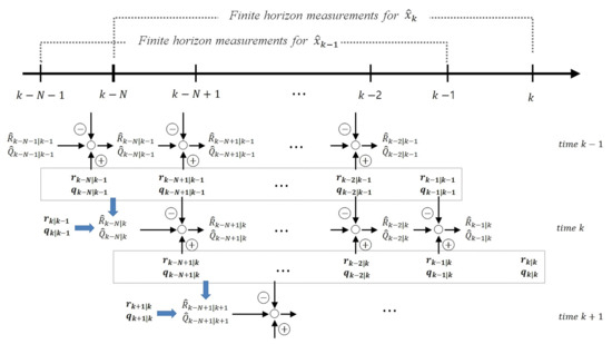
Figure 2. The concept of modified sequential noise statistics estimation in AFIR filter.

Firtly, consider the linear measurement state relationship to estimate the measurement noise statistics. On the horizon $[k-N-1k-1]$, i-th approximation sample of the measurement noise, $r_{k-N+i\mid k-1}$ can be represented as

$$\begin{array}{ccc}\hfill r_{k-N+i\mid k-1}& =& y_{k-N+i}-C_{k-N+i}{A}_{k-N+i}{\widehat{x}}_{k-N+i-1\mid k-1}.\hfill \end{array}$$

(53)

An unbiased estimate of the initial mean of the measurement noise at time k can be defined as

$$\begin{array}{c}\hfill {\widehat{r}}_{k-N\mid k}=\frac{1}{N}\sum _{i=1}^N{r}_{k-i+1\mid k-1},\end{array}$$

(54)

where $r_{k\mid k-1}=y_k-C_k{A}_k{\widehat{x}}_{k-1\mid k-1}$.

Then, the unbiased estimation of initial variance $C_{r,k-N\mid k}$ can be obtained as

$$\begin{array}{ccc}\hfill {\widehat{C}}_{r,k-N\mid k}& =& \frac{1}{N-1}\sum _{i=1}^N(r_{k-i\mid k-1}-{\widehat{r}}_{k-N\mid k}){(r_{k-i\mid k-1}-{\widehat{r}}_{k-N\mid k})}^T.\hfill \end{array}$$

(55)

By using the expectation of $C_{r,k-N\mid k}$ as

$$\begin{array}{c}\hfill E\left({\widehat{C}}_{r,k-N\mid k}\right)=\frac{1}{N}\sum _{i=1}^N{\gamma }_{k-i\mid k-1}+R_{k-N},\end{array}$$

(56)

the unbiased estimate of the initial measurement noise covariance ${\widehat{R}}_{k-N\mid k}$ can be obtained as

$$\begin{array}{ccc}\hfill {\widehat{R}}_{k-N\mid k}& =\hfill & \frac{1}{N-1}\sum _{i=1}^N((r_{k-i\mid k-1}-{\widehat{r}}_{k-N\mid k}){(r_{k-i\mid k-1}-{\widehat{r}}_{k-N\mid k})}^T\hfill \\ \hfill & \hfill & -\frac{N-1}{N}{\gamma }_{k-i\mid k-1}),\hfill \end{array}$$

(57)

where ${\gamma }_{k-i\mid k-1}=C_{k-i}{P}_{k-i\mid k-1}{C}_{k-i}^T$.

The mean and covariance of the measurement noise can be obtained on the horizon $[k-Nk]$ as

$$\begin{array}{ccc}\hfill {\widehat{r}}_{k-N+i\mid k}& =& {\widehat{r}}_{k-N+i-1\mid k}+\frac{1}{N}(r_{k-N+i\mid k}-r_{k-N+i\mid k-1}),\hfill \end{array}$$

(58)

$$\begin{array}{ccc}\hfill {\widehat{R}}_{k-N+i\mid k}& =\hfill & {\widehat{R}}_{k-N+i-1\mid k}+\frac{1}{N-1}((r_{k-N+i\mid k}-{\widehat{r}}_{k-N+i\mid k})\hfill \\ \hfill & \hfill & \times {(r_{k-N+i\mid k}-{\widehat{r}}_{k-N+i\mid k})}^T-(r_{k-N+i\mid k-1}-{\widehat{r}}_{k-N+i\mid k})\hfill \\ \hfill & \hfill & \times {(r_{k-N+i\mid k-1}-{\widehat{r}}_{k-N+i\mid k})}^T+\frac{1}{N}(r_{k-N+i\mid k}-r_{k-N+i\mid k-1})\hfill \\ \hfill & \hfill & \times {(r_{k-N+i\mid k}-r_{k-N+i\mid k-1})}^T-\frac{N-1}{N}({\gamma }_{k-N+i\mid k}-{\gamma }_{k-N+i\mid k-1})),\hfill \end{array}$$

(59)

for $1\le i\le N-1$. For $i=N$, ${\widehat{r}}_{k\mid k}$ and ${\widehat{R}}_{k\mid k}$ can be obtained by replacing $r_{k-N+i\mid k-1}$ and ${\gamma }_{k-N+i\mid k-1}$ in (58) and (59) with $r_{k-N\mid k-1}$ and ${\gamma }_{k-N\mid k-1}$, respectively.

Secondly, for the process noise statistics, define the approximation of state noise sample on the horizon $[k-N-1k-1]$ as

$$\begin{array}{ccc}\hfill q_{k-N+i\mid k-1}& =& {\widehat{x}}_{k-N+i\mid k-1}-A_{k-N+i}{\widehat{x}}_{k-N+i-1\mid k-1},\hfill \end{array}$$

(60)

where $q_{k-N+i\mid k-1}$ is defined as the i-th process noise sample at time k. In the same way as the process of measurement noise statistics, an unbiased estimate for horizon initial sampled mean ${\widehat{q}}_{k-N\mid k}$ at time k can be represented as

$$\begin{array}{ccc}\hfill {\widehat{q}}_{k-N\mid k}& =& \frac{1}{N}\sum _{i=1}^N{q}_{k-i+1\mid k-1},\hfill \end{array}$$

(61)

where $q_{k\mid k-1}={\widehat{x}}_{k\mid k-1}-A_k{\widehat{x}}_{k-1\mid k-1}$.

Then, the unbiased estimation of the initial process noise covariance ${\widehat{Q}}_{k-N\mid k}$ can be represented as

$$\begin{array}{ccc}\hfill {\widehat{Q}}_{k-N\mid k}& =\hfill & \frac{1}{N-1}\sum _{i=1}^N((q_{k-i\mid k}-{\widehat{q}}_{k-N\mid k}){(q_{k-i\mid k}-{\widehat{q}}_{k-N\mid k})}^T\hfill \\ \hfill & -\hfill & \frac{N-1}{N}{\mathsf{\Delta }}_{k-N+i\mid k-1}),\hfill \end{array}$$

(62)

where ${\mathsf{\Delta }}_{k-i\mid k-1}=A_{k-i}{P}_{k-i-1\mid k-1}{A}_{k-i}^T-P_{k-i\mid k-1}$. Then, the mean and covariance of the process noise on the horizon $[k-Nk]$ can be calculated sequentially as

$$\begin{array}{ccc}\hfill {\widehat{q}}_{k-N+i\mid k}& =& {\widehat{q}}_{k-N+i-1\mid k}+\frac{1}{N}(q_{k-N+i\mid k-1}-q_{k-N+i\mid k}),\hfill \end{array}$$

(63)

$$\begin{array}{ccc}\hfill {\widehat{Q}}_{k-N+i\mid k}& =\hfill & {\widehat{Q}}_{k-N+i-1\mid k}+\frac{1}{N-1}((q_{k-N+i\mid k}-{\widehat{q}}_{k-N+i\mid k})\hfill \\ \hfill & \hfill & \times {(q_{k-N+i\mid k}-{\widehat{q}}_{k-N+i\mid k})}^T-(q_{k-N+i\mid k-1}-{\widehat{q}}_{k-N+i\mid k})\hfill \\ \hfill & \hfill & \times {(q_{k-N+i\mid k-1}-{\widehat{q}}_{k-N+i\mid k})}^T+\frac{1}{N}(q_{k-i\mid k}-q_{k-i\mid k-1})\hfill \\ \hfill & \hfill & \times {(q_{k-i\mid k}-q_{k-i\mid k-1})}^T-\frac{N-1}{N}({\mathsf{\Delta }}_{k-N+i\mid k}-{\mathsf{\Delta }}_{k-N+i\mid k-1})),\hfill \end{array}$$

(64)

With the above sequential noise statistics esitmates, the AFIR filter can be obtained on the horizon $[k-Nk]$ as:

$$\begin{array}{ccc}\hfill {\widehat{x}}_{k-N+i+1\mid k}& =\hfill & A_{k-N+i}(I-K_{k-N+i}{C}_{k-N+i}){\widehat{x}}_{k-N+i\mid k}+A_{k-N+i}\hfill \\ \hfill & \hfill & \times K_{k-N+i}(y_{k-N+i}-{\widehat{r}}_{k-N+i\mid k})+{\widehat{q}}_{k-N+i\mid k},\hfill \end{array}$$

(65)

where the filter gain and prediction covariance matrix are obtained as

$$\begin{array}{ccc}\hfill K_{k-N+i}& =& P_{k-N+i\mid k}{C}_{k-N+i}^T{(C_{k-N+i}{P}_{k-N+i\mid k}{C}_{k-N+i}^T+{\widehat{R}}_{k-N+i\mid k})}^{-1},\hfill \end{array}$$

(66)

$$\begin{array}{ccc}\hfill P_{k-N+i+1\mid k}& =\hfill & A_{k-N+i}{P}_{k-N+i\mid k}{A}_{k-N+i}^T+{\widehat{Q}}_{k-N+i\mid k}-A_{k-N+i}{K}_{k-N+i}\hfill \\ \hfill & \hfill & \times (C_{k-N+i}{P}_{k-N+i\mid k}{C}_{k-N+i}^T+{\widehat{R}}_{k-N+i})K_{k-N+i}^T{A}_{k-N+i}^T,\hfill \end{array}$$

(67)

where the optimal unbiased estimate of the horizon initial state ${\widehat{x}}_{k-N\mid k}$ and the state covariance $P_{k-N\mid k}$ are obtained by (25) and (26) with estimated noise statistics ${\widehat{R}}_{·\mid k-1}$ and ${\widehat{Q}}_{·\mid k-1}$ in (59) and (64), respectively.

Since the noise statistics estimated in the AFIR filter are obtained by using the measurements a step ahead of the estimation time, the modified sequential noise statistics estimation method in the proposed AFIR filter may provide more adaptive estimation results than results given by previous sequential noise statistics estimation methods in adaptive Kalman filtering.

3. Simulation Results and Discussion

To demonstrate the validity of the proposed filters, the estimation performance of the proposed algorithms are compared with the conventional Kalman filter, modified Sage-Husa adaptive Kalman (SHAK) filters [22], and limited memory adaptive Kalman (LMAK) filter [23] for the F-404 gas turbine aircraft engine model in [19]. The discrete-time nominal F-404 gas turbine aircraft engine model can be represented as follows:

$$\begin{array}{ccc}\hfill x_{k+1}& =\hfill & A{x}_k+{\omega }_k\hfill \\ \hfill & =\hfill & \left[\begin{array}{ccc}0.9305& 0& 0.1107\\ 0.0077& 0.9802& -0.0173\\ 0.0142& 0& 0.8953\end{array}\right]x_k+w_k,\hfill \end{array}$$

(68)

$$\begin{array}{ccc}\hfill y& =\hfill & C{x}_k+v_k\hfill \\ \hfill & =\hfill & \left[\begin{array}{ccc}1& 0& 0\\ 0& 1& 0\end{array}\right]x_k+v_k,\hfill \end{array}$$

(69)

where covariances matrices of the process noise and measurement noise are set as $Q=0.02\ast I_{3\times 3}$ and $R=0.01\ast I_{2\times 2}$, respectively.

Even if dynamic systems and signals are well-represented in the state-space model, it may undergo unpredictable changes, such as jumps in frequency, phase, and velocity. These effects typically occur over a short time horizon, so they are called temporary uncertainties. Although these effects typically occur over a short time interval, the filter should be robust enough to diminish the effects of the temporary uncertainty. Due to its structure and measurement processing manner, an FIR estimator is believed to be robust against numerical errors and temporary modeling uncertainties that may cause a divergence phenomenon in the case of the IIR filter. To illustrate this fact and the fast convergence, the proposed filters and Kalman filter are compared for the following temporarily uncertain model, where temporary uncertainties are added to the nominal models (68) and (69), as

$$\begin{array}{ccc}\hfill x_{k+1}& =& \overline{A}{x}_k+{\overline{\omega }}_k=\left(A+\mathsf{\Delta }A\right)x_k+{\overline{\omega }}_k,\hfill \end{array}$$

(70)

$$\begin{array}{ccc}\hfill y& =& \overline{C}{x}_k+{\overline{v}}_k=\left(C+\mathsf{\Delta }C\right)x_k+{\overline{v}}_k,\hfill \end{array}$$

(71)

where

$$\begin{array}{c}\hfill \mathsf{\Delta }A=0.1{\delta }_k\ast I_{3\times 3},\mathsf{\Delta }C=\left[\begin{array}{ccc}0.01{\delta }_k& 0& 0\\ 0& 0.01{\delta }_k& 0\end{array}\right],{\delta }_k=\left\{\begin{array}{cc}1,& 200\le k\le 250,\\ 0,& otherwise,\end{array}\right.\end{array}$$

and process and measurement noise covariance matrices are taken as $\overline{Q}=0.25\ast I_{3\times 3}$ and $\overline{R}=0.02\ast I_{2\times 2}$, respectively.

Filters are designed for the nominal state-space models (68) and (69), then they are applied to the temporarily uncertain system (70) and (71). Additionally, the horizon length is taken as $N=15$ and $N=12$ for the proposed FIR filters and LMAK filter, respectively, and the forgetting factor of SHAK filter is set as $\alpha =0.3$.

Figure 3, Figure 4 and Figure 5 show estimation errors for the states $x_1$, $x_2$, and $x_3$, respectively, for five filters. In addition, mean relative estimation errors (MREE) are also compared in Table 1, Table 2 and Table 3. The MREE is defined as

$$\begin{array}{c}\hfill e_r=\frac{1}{N_f-N_s}\sum _{k=N_s}^{N_f}\frac{|x_k-{\widehat{x}}_k|}{\left|\frac{1}{N_f-N_s}{\sum }_{k=N_s}^{N_f}{x}_k\right|},\end{array}$$

(72)

where $x_k$ is the real state, ${\widehat{x}}_k$ is the estimate of the filter, $N_s$ and $N_f$ are the initial time and the end time of simulation, respectively.

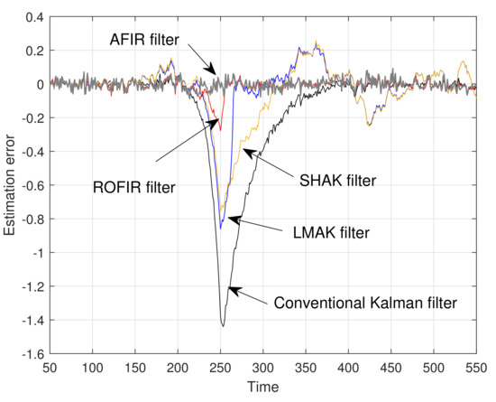
Figure 3. Estimation error for the first state $x_{1,k}$ ($e_{1,k}=x_{1,k}-{\widehat{x}}_{1,k}$).

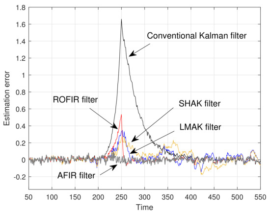
Figure 4. Estimation error for the second state $x_{2,k}$ ($e_{2,k}=x_{2,k}-{\widehat{x}}_{2,k}$).

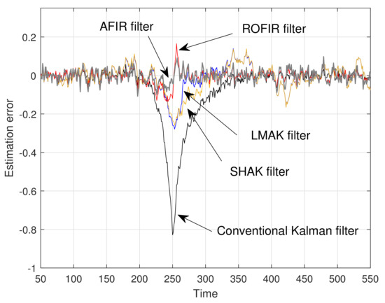
Figure 5. Estimation error for the third state $x_{3,k}$ ($e_{3,k}=x_{3,k}-{\widehat{x}}_{3,k}$).

Table 1. Comparison of the MREE for the first state ($e_{1,r}$).

Time Interval	$\left[50550\right]$	$\left[50200\right]$	$\left[201400\right]$	$\left[401550\right]$
Kalman filter	$0.7567$	$0.2157$	$2.6138$	$0.1789$
SHAK filter	$0.4107$	$0.4852$	$1.3432$	$0.7997$
LMAK filter	$0.3760$	$0.4394$	$1.2185$	$0.7809$
ROFIR filter	$0.1038$	$0.2469$	$0.3141$	$0.1965$
AFIR filter	$0.0872$	$0.2927$	$0.1546$	$0.2476$

Table 2. Comparison of the MREE for the second state ($e_{2,r}$).

Time Interval	$\left[50550\right]$	$\left[50200\right]$	$\left[201400\right]$	$\left[401550\right]$
Kalman filter	$0.2709$	$0.1933$	$0.4839$	$0.1579$
SHAK filter	$0.0642$	$0.2431$	$0.0998$	$0.5697$
LMAK filter	$0.0558$	$0.2387$	$0.0894$	$0.4248$
ROFIR filter	$0.0552$	$0.2314$	$0.0947$	$0.1779$
AFIR filter	$0.0216$	$0.2490$	$0.0240$	$0.2011$

Table 3. Comparison of the MREE for the third state ($e_{3,r}$).

Time Interval	$\left[50550\right]$	$\left[50200\right]$	$\left[201400\right]$	$\left[401550\right]$
Kalman filter	$0.7973$	$0.3574$	$3.3627$	$0.2304$
SHAK filter	$0.3510$	$0.6860$	$1.2738$	$0.6468$
LMAK filter	$0.3355$	$0.6675$	$1.2022$	$0.6429$
ROFIR filter	$0.1808$	$0.4205$	$0.6386$	$0.2776$
AFIR filter	$0.1756$	$0.5891$	$0.4568$	$0.4040$

Since the conventional Kalman filter provides optimal estimates, the estimation errors of the conventional Kalman filter are smaller than those of other filters during the time interval $\left[50200\right]$, when there are no system uncertainties. However, from the simulation results in time intervals $\left[50550\right]$ and $\left[201400\right]$, it can be seen that the proposed ROFIR and AFIR filters have smaller estimation errors and faster convergence speed than the conventional Kalman filter and adaptive Kalman filters. These results show that when model uncertainties exist, the proposed ROFIR and AFIR filters can work well and have better performance than the Kalman filters due to their FIR structure.

By comparing the simulation results of adaptive filters in time interval $\left[201400\right]$, it can be easily shown that the estimation errors of the proposed AFIR filter are remarkably smaller than those of LMAK filter, even though the horizon length of the proposed AFIR filter is larger than that of LMAK filter. In addition, the estimation errors of the proposed AFIR filter rapidly converge to zero after temporary model uncertainty disappears, whereas those of adaptive Kalman filters do not. Moreover, the estimation errors of adaptive Kalman filters fluctuate and oscillate during time interval $\left[401550\right]$, which are caused by accumulation of estimation errors. From these results, it can be assumed that the modified sequential noise statistics estimation method and its combination with recursive FIR filtering make for more adaptive and faster convergence performance than the sequential noise statistics estimation with Kalman filtering.

4. Conclusions

In this paper, the optimal- and recursive-form FIR filter was proposed by employing the Kalman filtering technique, moving the horizon estimation strategy for discrete time-varying state-space models. The initial state and its error covariance were optimally estimated in the maximum likelihood sense over the horizon, then they initiated the finite horizon Kalman filter. The proposed recursive optimal FIR filter was designed without assumption of nonsingular transition system matrix and any a priori initial information. In addition, it was also proved that the proposed ROFIR filter is the best linear estimator on the finite estimation horizon. Furthermore, by applying the modified sequential noise statistics estimation method to the ROFIR filter, an AFIR filter was also proposed as an application of the ROFIR filter, which shows that many useful techniques of Kalman filtering could be applied to the proposed ROFIR filter for improving the estimation performance of FIR filters. To validate the proposed filters, computer simulation was performed and it was shown that the proposed filters were more accurate and robust than other conventional Kalman filters and adaptive Kalman filters.

References

- Fitzgerald, R.J. Divergence of the Kalman filter. IEEE Trans. Autom. Control 1971, 6, 736–747. [Google Scholar] [CrossRef]
- Sangsuk-Iam, S.; Bullock, T.E. Analysis of discrete-time Kalman filtering under incorrect noise covariances. IEEE Trans. Autom. Control 1990, 35, 1304–1309. [Google Scholar] [CrossRef]
- Grewal, M.S.; Anderews, A.P. Kalman Filtering—Theory and Practice; Prentice-Hall: Englewood Cliffs, NJ, USA, 1993. [Google Scholar]
- Kwon, W.H.; Lee, K.S.; Kwon, O.K. Optimal FIR Filters for Time-Varying State-Space Models. IEEE Trans. Aerosp. Electron. Syst. 1990, 26, 1011–1021. [Google Scholar] [CrossRef]
- Kwon, B.; Quan, Z.; Han, S. A robust fixed-lag receding horizon smoother for uncertain state space models. Int. J. Adapt. Control Signal Process. 2015, 29, 1354–1366. [Google Scholar] [CrossRef]
- Kwon, B.; Han, S.; Han, S. Improved Receding Horizon Fourier Analysis for Quasi-periodic Signals. J. Electr. Eng. Technol. 2017, 12, 378–384. [Google Scholar] [CrossRef]
- Kwon, W.H.; Kim, P.S.; Park, P. A receding horizon Kalman FIR filter for discrete time-invariant systems. IEEE Trans. Autom. Control 1999, 44, 1787–1791. [Google Scholar] [CrossRef]
- Kwon, W.H.; Kim, P.S.; Han, S.H. A Receding Horizon Unbiased FIR Filter for Discrete-Time State Space Models. Automatica 2002, 38, 545–551. [Google Scholar] [CrossRef]
- Shmaliy, Y.S.; Munoz-Diaz, J.; Arceo-Miquel, L. Optimal horizons for a one-parameter family of unbiased FIR filter. Digit. Signal Process. 2008, 18, 739–750. [Google Scholar] [CrossRef]
- Shmaliy, Y.S. An iterative Kalman-like algorithm ignoring noise and initial conditions. IEEE Trans. Signal Process 2011, 59, 2465–2473. [Google Scholar] [CrossRef]
- Kou, Y.; Jiao, Y.; Xu, D.; Zhang, M.; Liu, Y.; Li, X. Low-cost precise measurement of oscillator frequency instability based on GNSS carrier observation. Adv. Space Res. 2012, 51, 969–977. [Google Scholar] [CrossRef]
- Pak, J.M.; Ahn, C.K.; Shmaliy, Y.S.; Shi, P.; Lim, M.T. Switching extensible FIR filter bank for adaptive horizon state estimation with application. IEEE Trans. Control Syst. Technol. 2016, 24, 1052–1058. [Google Scholar] [CrossRef]
- Shmaliy, Y.S.; Khan, S.; Zhao, S. Ultimate iterative UFIR filtering algorithm. Measurement 2016, 92, 236–242. [Google Scholar] [CrossRef]
- Zhao, S.; Shmaliy, Y.S.; Liu, F. Fast Kalman-Like Optimal Unbiased FIR Filtering with Applications. IEEE Trans. Signal Process. 2016, 64, 2284–2297. [Google Scholar] [CrossRef]
- Zhao, S.; Shmaliy, Y.S.; Ahn, C.K.; Liu, F. Adaptive-Horizon Iterative UFIR Filtering Algorithm with Applications. IEEE Trans. Ind. Electron. 2018, 65, 6393–6402. [Google Scholar] [CrossRef]
- Zhao, S.; Shmaliy, Y.S.; Ahn, C.K.; Liu, F. Self-Tuning Unbiased Finite Impulse Response Filtering Algorithm for Processes with Unknown Measurement Noise Covariance. IEEE Trans. Control Syst. Technol. 2021, 29, 1372–1379. [Google Scholar] [CrossRef]
- Pak, J.M.; Yoo, S.Y.; Lim, M.T.; Song, M.K. Weighted Average Extended FIR Filter Bank to Manage the Horizon Size in Nonlinear FIR Filtering. Int. J. Control Autom. Syst. 2014, 13, 138–145. [Google Scholar] [CrossRef]
- Pak, J.M.; Kim, P.S.; You, S.H.; Lee, S.S.; Song, M.K. Extended Least Square Unbiased FIR Filter for Target Tracking Using the Constant Velocity Motion Model. Int. J. Control Autom. Syst. 2017, 15, 947–951. [Google Scholar] [CrossRef]
- Kim, P.S. Selective Finite Memory Structure Filtering Using the Chi-Square Test Statistic for Temporarily Uncertain Systems. Appl. Sci. 2019, 9, 4257. [Google Scholar] [CrossRef]
- Kwon, B.; Han, S.; Lee, K. Robust Estimation and Tracking of Power System Harmonics Using an Optimal Finite Impulse Response Filter. Energies 2018, 11, 1811. [Google Scholar] [CrossRef]
- Kwon, B. An Optimal FIR Filter for Discrete Time-varying State Space Models. J. Inst. Control Robot. Syst. 2011, 17, 1183–1187. [Google Scholar] [CrossRef][Green Version]
- Akhlaghi, S.; Zhou, N.; Huang, Z. Adaptive Adjustment of Noise Covariance in Kalman Filter for Dynamic State Estimation. In Proceedings of the 2017 IEEE Power and Energy Society General Meeting, Chicago, IL, USA, 16–20 July 2017. [Google Scholar]
- Myers, K.; Tapley, B. Adaptive sequential estimation with unknown noise statistics. IEEE Trans. Autom. Control 1976, 21, 520–523. [Google Scholar] [CrossRef]
Publisher’s Note: MDPI stays neutral with regard to jurisdictional claims in published maps and institutional affiliations. |
© 2022 by the authors. Licensee MDPI, Basel, Switzerland. This article is an open access article distributed under the terms and conditions of the Creative Commons Attribution (CC BY) license (https://creativecommons.org/licenses/by/4.0/).