Data-Driven Adaptive Equivalent Consumption Minimization Strategy for Hybrid Electric and Connected Vehicles

Abstract

Advanced energy management strategies (EMS) are used to control the power flow through a vehicle’s powertrain. However, the cost of high-power computational hardware and lack of a priori knowledge of future road conditions poses difficult challenges for engineers attempting to implement globally optimal frameworks. One solution is to use advanced driver assistance systems (ADAS) and connectivity to obtain a prediction of future road conditions. This paper presents a look-ahead predictive EMS which combines approximate dynamic programming (ADP) methods and an adaptive equivalent consumption minimization strategy (A-ECMS) to obtain a near-optimal solution for a future prediction horizon. ECMS is highly sensitive to the equivalence factor (EF), making it necessary to adapt during a trip to account for disturbances. A novel adaptation method is presented in this work which uses an artificial neural network to learn the nonlinear relationship between a speed and the state of charge (SOC) trajectory prediction obtained from ADP to estimate the corresponding EF. A traffic uncertainty analysis demonstrates an approximately 10% fuel economy (FE) improvement over traditional A-ECMS. Using a data-driven adaptation method for A-ECMS informed by a dynamic programming (DP) based prediction results in an EMS capable of online implementation.

1. Introduction

Government regulations worldwide are pushing toward clean, renewable energy to reduce pollution levels and create a sustainable future. In response, the automotive industry has invested heavily in innovative technology such as electrified powertrains. Electrification of powertrains provides attractive benefits over conventional powertrains, including engine downsizing, electric motor assist, and engine start-stop. Similarly, the automation of driving promises safer driving; hence, the automotive industry is embracing connected and automated vehicle (CAV) technology. A CAV uses advanced on-board sensing technology to obtain information about surroundings (commonly referred to as look-ahead data) and make informed decisions about present and future actions. Perception and control algorithms, such as sensor fusion and adaptive cruise control (ACC), leverage this information to make vehicles safer and more efficient.

The integration of electrification and driving automation has the potential of extending the benefits of both these technologies. However, the additional degrees of freedom result in a complex system which demands more advanced control methods. To achieve maximum powertrain efficiency, researchers and automotive manufacturers have dedicated significant effort to the development and advancement of energy management strategies (EMS) [1]. For hybrid electric vehicle (HEV) powertrain control, an EMS is a set of algorithms that decide the power split between the internal combustion engine and the EM. The goal of the EMS is to improve fuel economy (FE) and optimize the performance of HEVs [2]. In [3], a discrete dynamic programming (DP) approach is used to optimize torque split, gear shifting, and velocity trajectory for a parallel HEV. A model predictive controller (MPC) is used in [4] to optimize the velocity profile and torque split with a gradient-based optimization. In [5], DP with an underlying adaptive equivalent consumption minimization strategy (ECMS) is used to optimize torque split and velocity trajectory. Although energy management of HEVs and CAVs has been the focus of many recent publications, the use of look-ahead data for optimal energy management remains an open research topic.

A key component of a look-ahead EMS is the use of vehicle-to-everything (V2X) communication. The authors in [6,7] showed how vehicle-to-infrastructure (V2I) and GPS signals can be used as inputs to a perception model to employ an artificial neural network (ANN) to characterize driving patterns in an optimal EMS for a plug-in HEV (PHEV). A traffic model was applied in [8] to predict future vehicle velocity with vehicle-to-vehicle (V2V) and V2I as inputs, and an optimal EMS was derived using Pontryagin’s minimum principle (PMP). In [9], traffic light signal phase and timing (SPaT) was used to give dynamic speed advice to the driver and demonstrated a FE improvement of 12–14%.

Although the main focus of recent development in optimal energy management has been on look-ahead data-based optimal control, the key concern stems from the computational requirements of global optimization algorithms. The implementation of global optimization algorithms on microprocessors available on board a typical passenger car is challenging due to various reasons, including the high cost of hardware [1]. Research programs such as FutureTruck, EcoCAR, and NEXTCAR were designed to address these issues. A team of students and faculty at Ohio State University (OSU) implemented ECMS on a model-year 2000 Chevrolet Suburban SUV as part of the FutureTruck 2000 competition and achieved approximately 1.5 times the FE of the production Suburban [10]. More recently, the OSU NEXTCAR team implemented a model predictive control framework on a test vehicle using principles of approximate dynamic programming (ADP) with various look-ahead data sources. Real-world testing was conducted on a test track and resulted in more than 20% FE improvement over the base vehicle control strategy [11].

Many different methods to overcome the challenges of implementing global optimization algorithms are proposed in the literature. In [12], a DP-based EMS is used in a predictive control scheme to feed a conventional cruise controller with new set points on a heavy duty truck. The authors demonstrate real-world fuel consumption reduction for highway driving. In [13], DP optimization is done using cloud computing for optimizing the velocity reference that is tracked by a human driver. The authors of [14] reduced computational cost by separately formulating the car-following control and energy management strategy and then coupling the control laws in a MPC framework. Online implementation was demonstrated in hardware-in-the-loop experiments.

In recent studies, the authors in [15] proposed an intelligent ECMS, where a Bayesian regularization neural network was used to predict the near-optimal equivalence factor (EF), and a back propagation neural network was used to forecast the engine on/off state to improve the quality of the EF prediction. In [16], a two-layer strategy was used where the upper layer extracts trip and vehicle information using CAV technology and solves DP on a remote server. The lower level controller was based on Q-learning and was used for real-time implementation of the optimal result obtained from DP. In [17], the authors developed a hybrid deep Q-learning and policy gradient method for vehicles driving along multi-lane urban signalized corridors to learn well-established longitudinal fuel-saving strategies. Numerical experiments demonstrate up to a 46% fuel reduction compared to their baseline model. The authors of [18] proposed a look-ahead horizon-based co-optimization of vehicle dynamics and powertrain operation to minimize energy consumption with the constraint of driving safety to avoid traffic collisions. The optimal solution was derived by PMP and verified in a traffic-in-the-loop simulation environment.

Most of the past literature assumes no stochastic uncertainties in the prediction of future events. However, with existing hardware limitations, it is unrealistic to implement the stochastic optimal control methods. The current work proposes a method of using CAV technology to improve the energy efficiency of HEVs with a clear path to on-board implementation. The novelty of the work lies in the approach that combines machine learning, optimal control and traditional ECMS and concurrently optimizes the vehicle speed profile as well as EMS. The proposed approach is computationally efficient and provides better FE gains than ECMS. The primary objective is to quantify the potential for FE improvements using a look-ahead predictive EMS. An approach is outlined for using look-ahead data to obtain a prediction of future vehicle state trajectories (e.g., vehicle speed and battery state of charge) for a single vehicle using a DP-based rollout algorithm. A novel EF adaptation technique for ECMS is introduced, and the effect of traffic uncertainty on FE is measured through statistical methods. In a simulation study, we demonstrate about $10\%$ FE gains over a baseline consisting of a combination of A-ECMS and the intelligent driver model. Recently, an MPC-based approach was shown to provide $20\%$ FE gains over a rule-based EMS [11] but required higher computation time. Considering that the baseline in [11] was inferior to A-ECMS and required more computational resources, the FE gains obtained in this study are significant.

The remainder of this paper first outlines the modeling framework and methodology used to formulate the proposed EMS. This is followed by a discussion of simulation results and key findings. Finally, a conclusion of the study is provided.

2. Materials and Methods

This section begins with the general architecture of the proposed EMS. The vehicle architecture and modelling used throughout this study are then described. Each block of the EMS is then explained in detail.

2.1. Proposed Architecture of EMS

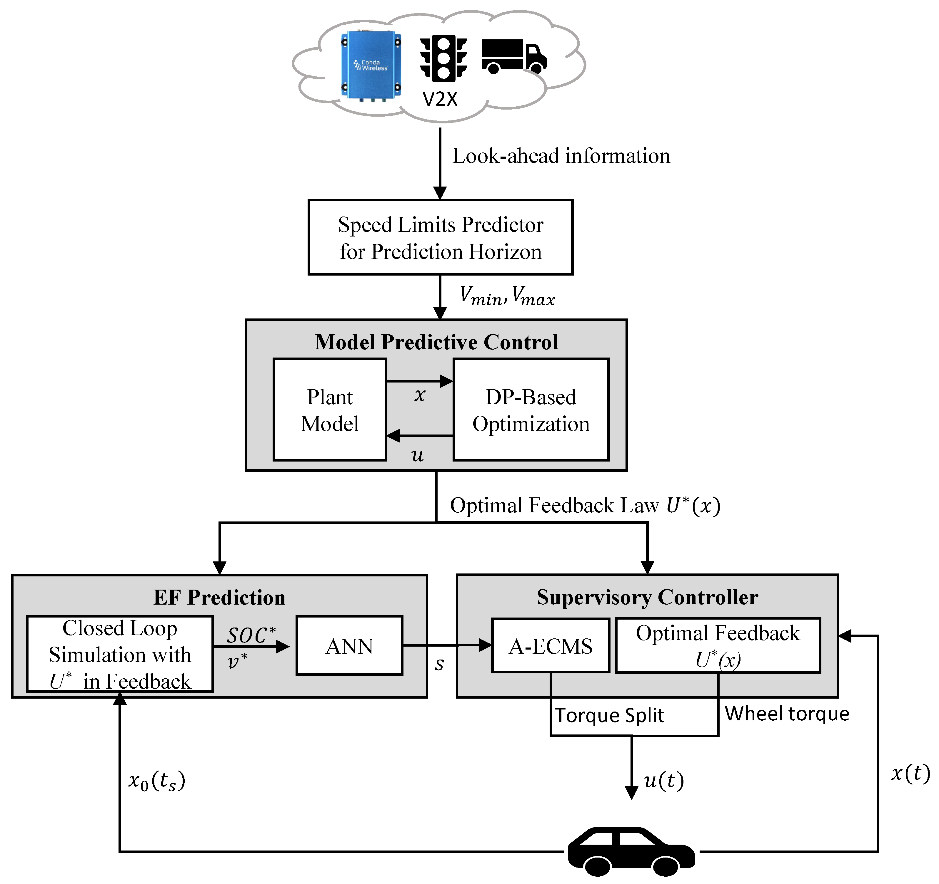
The overall structure of the EMS presented in this paper, referred to as DP-ECMS, is shown in Figure 1. It relies on principles of optimal control to minimize fuel consumption considering look-ahead data. For this research, look-ahead data is a combination of traffic flow control devices (i.e., traffic light location and SPaT, stop signs) and road characteristics (i.e., speed limits, average traffic flow speed) obtained from sensors, including radar, camera, dedicated short range communication (DSRC), and GPS. All the look-ahead data is simulated and therefore assumed to be available at all times with no delays in data transmission. All modeling and simulation in this study is done using MATLAB and Simulink R2019b.

Look-ahead data is used to obtain a speed limit prediction for the ego vehicle based on upcoming road conditions. This is done by layering different look-ahead data sources and finding the maximum safe speed. The average traffic flow speed is first compared to the legal speed limit. The effective speed limit is taken to be the minimum of the two. If the vehicle is in range of a connected intersection, SPaT is used to determine if the vehicle can pass on green. A simple rule-based method is used to find the speed needed to pass during a green window, where the speed is calculated by dividing the distance to the traffic light by the time left in the current phase. If the speed to pass on green does not violate the bounds set by traffic or the legal speed limit, it is taken as the effective speed limit. If speed constraints are violated, the effective speed limit at the traffic light is set to zero and the vehicle will be forced to stop. If there is no traffic and no traffic lights, the effective speed limit is simply the legal speed limit.

The EMS shown in Figure 1 uses a modular control structure, which can be broken down into three key phases: the rollout algorithm-based MPC, a supervisory control and an EF predictor. The MPC uses the future speed limits obtained from the road data, SPaT and traffic to optimize the vehicle speed and battery SOC. It generates an optimal feedback control law for each control input, namely the total wheel torque and the torque split between the EM and internal combustion (IC) engine. The nonlinear MPC that uses DP as a solver cannot be executed at the rate of the powertrain controller due to computation time limitations. Additionally, the feedback law is not robust to stochastic uncertainties due to traffic. Hence, a supervisory controller is designed that uses the optimal feedback law obtained from nonlinear MPC in combination with adaptive ECMS. The supervisory controller uses the optimal feedback law to compute total wheel torque, but uses ECMS to compute the torque split ratio. Since there is no optimization in the supervisory controller, it can be executed at the rate of a typical powertrain controller. The key issue is that the ECMS requires an optimal equivalency factor that depends on the speed profile. Hence, a data-driven EF predictor is used which is based on the optimal speed and SOC trajectories obtained from a closed-loop simulation over the prediction horizon. An ANN is trained to generate an optimal EF for the expected future speed profile. It should be noted that all three phases are executed at different time rates. The supervisory controller is executed at the rate of 100 Hz. The MPC is executed once every 10 s, and the EF prediction is executed once every 30 s.

2.2. Powertrain Model

The work presented in this paper is motivated by the EcoCAR Mobility Challenge (MC) competition objectives and is designed to serve as the primary energy management system for the OSU competition vehicle. 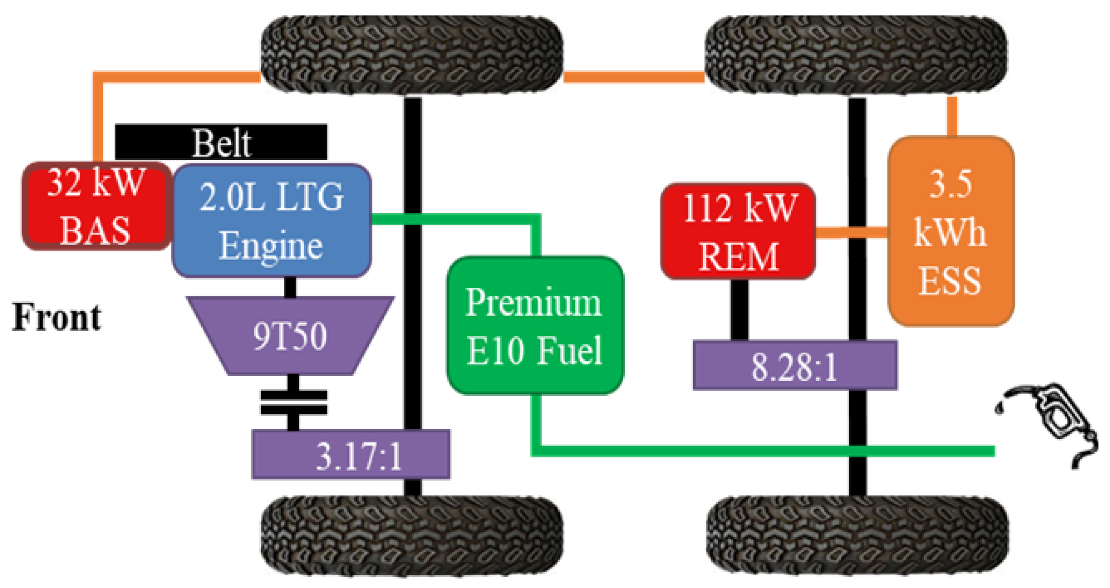EcoCAR MC is a 4-year competition which challenges university students to apply advanced propulsion systems, electrification, SAE Level 2 automation, and vehicle connectivity to improve the energy efficiency, safety and consumer appeal of the competition-provided vehicle [19]. The vehicle in consideration is a 2019 Chevrolet Blazer with a through-the-road parallel hybrid architecture consisting of a General Motors (GM) 2.0 L turbocharged gasoline engine coupled with a DENSO 32 kW belted alternator-starter (BAS) for front powertrain propulsion and a 90 kW Parker Hannifin GVM210-100 electric machine mated to a BorgWarner eGearDrive rear-axle single speed gearbox to power the rear axle. A custom 3.5 kW-h Li-ion battery pack provided by Hybrid Design Services (HDS) serves as the electrical energy storage system (ESS). The vehicle powertrain architecture is highlighted in Figure 2.

In this paper we assume SI units for all model parameters. For powertrain energy analysis, it is sufficient to model the vehicle as a point mass and express longitudinal dynamics as the equilibrium of forces acting on the vehicle. The equation of motion for a point mass can be derived from the equilibrium of forces acting on a vehicle:

$$\begin{array}{c}{M}_{veh}\frac{d{v}_{veh}}{dt}=\frac{T_{pwt}-T_{brake}}{R_{wh}}-c_{roll}{M}_{veh}gcos\delta -\frac{1}{2}{\rho }_{air}{A}_f{C}_d{v}_{veh}^2-M_{veh}gsin\delta \end{array}$$

(1)

where $M_{veh}$ is the effective vehicle mass, $v_{veh}$ is the longitudinal vehicle velocity, ${\rho }_{air}$ is the air density, $A_f$ is the vehicle frontal area, $C_d$ is the aerodynamic coefficient, g is the gravity acceleration, $\delta$ is the road slope angle, $c_{roll}$ is the rolling resistance coefficient, $T_{pwt}$ is the torque generated at the wheel shaft by the powertrain, $T_{brake}$ is the braking torque, and $R_{wh}$ is the wheel radius. Wheel speed is calculated using:

$$\begin{array}{c}{\omega }_{wh}=\frac{v_{veh}}{R_{wh}}.\end{array}$$

(2)

A simple transmission model is used which assumes a constant efficiency term:

$$\begin{array}{c}{\omega }_t=g_t{\omega }_{wh}\end{array}$$

(3)

$$T_t=\left\{\begin{array}{cc}\frac{{\eta }_t}{g_t}{T}_{wh}\hfill & \mathrm{if}{P}_{wh}=T_{wh}·{\omega }_{wh}\ge 0,\hfill \\ \frac{1}{{\eta }_t{g}_t}{T}_{wh}\hfill & \mathrm{if}{P}_{wh}=T_{wh}·{\omega }_{wh}<0\hfill \end{array}\right.$$

(4)

where ${\omega }_t$ is the transmission speed, $g_t$ is the transmission gear ratio, $T_t$ is the transmission torque, ${\eta }_t$ is the transmission efficiency, and $T_{wh}$ is the wheel torque, which is equal to the force at the wheels multiplied by the wheel radius.

A simple torque converter model is based on lookup tables created with experimental data for the pump and turbine torque ratio, capacity factor ($K_{tc}$), and speed ratio. The internal combustion engine model uses a static map-based approach which assumes that the engine is a perfect actuator with no response delays. Fuel consumption is calculated using an engine fuel map which is a function of engine speed and torque:

$$\begin{array}{c}{\dot{m}}_f=f_{FE}({\omega }_{ice},T_{ice})\end{array}$$

(5)

where ${\dot{m}}_f$ is the fuel flow rate, ${\omega }_{ice}$ is the engine speed, and $T_{ice}$ is the engine torque.

The rear electric motor (REM) uses a static map model based on torque and efficiency maps. The REM is treated as a perfect actuator where transient effects are assumed to be captured by the map. The governing equations, in terms of power, for the REM model are as follows:

$$P_{elec}=\left\{\begin{array}{cc}\frac{1}{{\eta }_{rem}({\omega }_{rem},P_{elec})}{\omega }_{rem}{T}_{rem}\hfill & \mathrm{if}{P}_{elec}\ge 0(\mathrm{motoring}\mathrm{mode}),\hfill \\ {\eta }_{rem}({\omega }_{rem},P_{elec})·{\omega }_{rem}{T}_{rem}\hfill & \mathrm{if}{P}_{elec}<0(\mathrm{generating}\mathrm{mode})\hfill \end{array}\right.$$

(6)

where ${\eta }_{rem}$, ${\omega }_{rem}$, and $T_{rem}$ are the REM efficiency, REM speed, and REM torque, respectively.

The battery pack is modeled by a 0^th order equivalent circuit model (ECM). SOC dynamics are given by:

$$\dot{SOC}\left(t\right)=\left\{\begin{array}{cc}\frac{-1}{{\eta }_{coul}}\frac{I\left(t\right)}{Q_{nom}}\hfill & \mathrm{if}I\left(t\right)>0\hfill \\ -{\eta }_{coul}\frac{I\left(t\right)}{Q_{nom}}\hfill & \mathrm{if}I\left(t\right)<0\hfill \end{array}\right.$$

(7)

where $Q_{nom}$ is the nominal charge capacity, I is the battery current and ${\eta }_{coul}$ is the Coulombic efficiency. The circuit equation, as a function of terminal power, is:

$$\begin{array}{c}{P}_{batt}=V_L·I=V_{OC}I-R_0{I}^2\end{array}$$

(8)

where $P_{batt}$ is the battery power, $V_L$ is the load voltage at the battery terminals, $V_{OC}$ is the open circuit voltage, and $R_0$ is the internal resistance. Accessory and auxiliary loads are assumed to be constant and modeled as a constant current draw from the battery pack. An explicit expression of current as a function of power is obtained:

$$\begin{array}{c}I=\frac{V_{OC}}{2R_0}-\sqrt{{\left(\frac{V_{OC}}{2R_0}\right)}^2-\frac{P_{batt}}{R_0}}.\end{array}$$

(9)

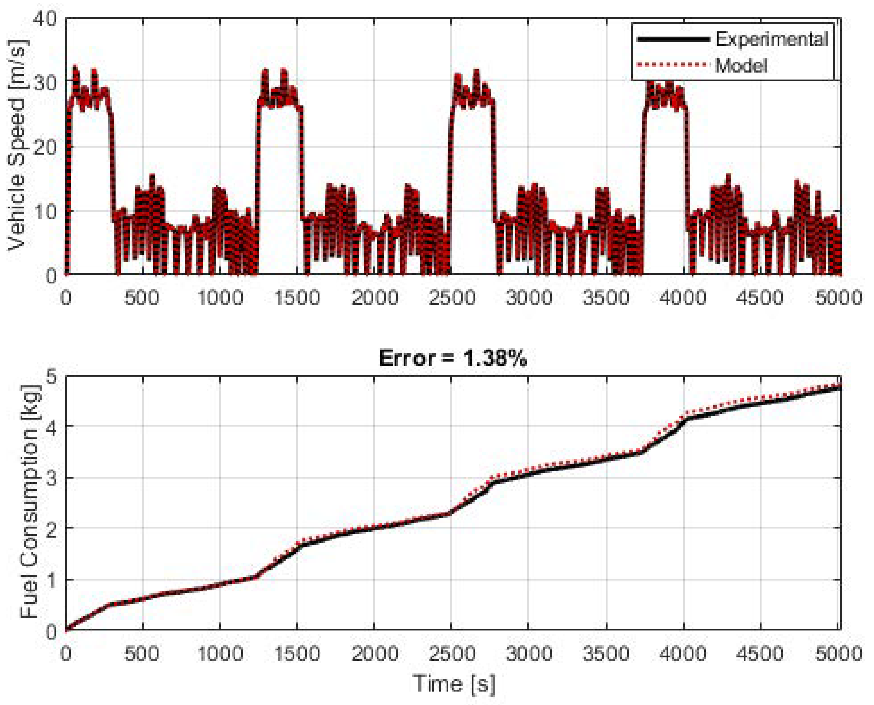
To validate model accuracy, the test vehicle was run over a team-developed drive cycle at the Transportation Research Center (TRC) in East Liberty, Ohio. Data were collected at a rate of 50 Hz using a dSPACE MicroAutoBox II with dSPACE experiment software, ControlDesk. Vehicle speed was obtained from the wheel speed sensor signal and fuel consumption from the fuel flow rate read from the engine control unit (ECU). Figure 3 shows the drive cycle and a comparison of the total fuel consumption. The final fuel consumption value obtained from the simulation is 1.38% higher than the experimental data, indicating that the model closely matches the test vehicle.

2.3. Nonlinear Model Predictive Control

The objective is to minimize fuel consumption as well as travel time. A rollout algorithm that is based on the concept of MPC is chosen due to the feedback inherently present in the controller architecture. Utilizing MPC allows the optimal policy to be updated at each time step. The feedback control structure and frequent updates add robustness to uncertainties in the predictions. DP is chosen as the optimization algorithm due to its ability to handle nonlinear constraints and its guaranteed optimal solution, given information about the road segment in the look-ahead horizon. The length of the look-ahead horizon is a design choice and a trade-off between computation time and optimality. A smaller look-ahead horizon has fewer steps, and hence is computationally more efficient, whereas a longer horizon uses more future information but requires more time to compute.

Assume that at time instance t the vehicle is at distance n from the origin. At this instance, using the future speed limits, DP provides the optimal feedback law $U^{*}$ for the segment of horizon length $N_h$. The optimal feedback controller is re-computed using DP at the update rate of 10 s.

Most of the look-ahead data (speed limits, SPaT, stop signs, etc.) are static, i.e., the location of these data sources is fixed with respect to the distance along the route, and they do not vary with time. For this reason, the optimal control problem is expressed in terms of distance as opposed to time. The objective function for MPC is a convex combination of fuel consumption and travel time.

At any distance step n along the route, the objective function can be written as:

$$\begin{array}{c}J=\underset{u_i\in U_i}{min}G\left(x_{n+N_h}\right)+\sum _{i=n}^{n+N_h}\left(\beta ·\frac{{\dot{m}}_{f,i}(x_i,u_i)}{{\dot{m}}_{f,norm}}+(1-\beta )\right)·\frac{\Delta s_i}{V_{veh,i}}\end{array}$$

(10)

where n is the first step (distance) for the current horizon at time j, $N_h$ is the horizon length, $\beta \in [0,1]$ represents the trade-off between fuel consumption and travel time, $\Delta s_i$ is the distance traveled over one step, ${\dot{m}}_{f,i}$ is the fuel flow rate, ${\dot{m}}_{f,norm}$ is a normalizing factor, $x_i={\left[\begin{array}{cc}{V}_{veh,i}& SO{C}_i\end{array}\right]}^T$ is the state vector, $u_i={\left[\begin{array}{cc}{T}_{whl,i}& {\tau }_i\end{array}\right]}^T$ is the control input vector, $V_{veh,i}$ is the vehicle speed, G is the terminal cost at distance $n+N_h$, and ${\tau }_i$ is the torque split ratio between REM torque and IC engine torque. Since the aim of this research is energy management, metrics such as driver comfort and tail pipe emissions are not explicitly considered in the objective function. The objective function is subject to the following constraints:

$$\begin{array}{c}\hfill \begin{array}{cc}\hfill SO{C}_{min}& \le SO{C}_i\le SO{C}_{max}\hfill \\ \hfill \left(V_{veh,min,i}\right){|}_n& \le V_{veh,i}\le \left(V_{veh,max,i}\right){|}_n\hfill \\ \hfill T_{ice,min}& \le T_{ice,i}\le T_{ice,max}\hfill \\ \hfill T_{rem,min}& \le T_{rem,i}\le T_{rem,max}\hfill \\ \hfill x_{i+1}& =f(x_i,u_i,\Delta s_i)\hfill \end{array}\end{array}$$

(11)

where $SO{C}_{min}$, $SO{C}_{max}$ and $SO{C}_i$ are the minimum, maximum, and current state of charge, respectively, $\left(V_{veh,min,i}\right){|}_n$ and $\left(V_{veh,max,i}\right){|}_n$ are the minimum and maximum allowable speeds determined from look-ahead data obtained when the vehicle is at distance n, $V_{veh,i}$ is current vehicle speed, $T_{ice,min}$,$T_{ice,max}$, $T_{ice,i}$, $T_{rem,min}$, $T_{rem,max}$, and $T_{rem,i}$ are the minimum, maximum, and current engine torque and REM torque, respectively, and f is the discrete powertrain model. The powertrain model is equivalently expressed such that the independent variable of the difference equation is distance and not time.

For the rollout algorithm, the terminal cost $G\left(x_{n+N_h}\right)$ in Equation (10) can be determined using a base policy. The method chosen for this work is based on the principles of approximate DP where a base policy is used to approximate the terminal cost in Equation (10). The base policy is obtained by solving the optimal control problem for the entire route with the speed limits available at the beginning of the trip. The full route optimal control problem is the same as described by Equations (10) and (11) but with $n=0$ and $N_h=N$, where N is the total number of steps for the full route. The terminal cost $G\left(x_N\right)$ is such that the SOC at the end of the trip is equal to the SOC at the start of the trip, i.e.,

$$G\left(x_N\right)=\left\{\begin{array}{cc}0\hfill & SO{C}_N=SO{C}_0\hfill \\ inf\hfill & otherwise\hfill \end{array}\right.$$

(12)

where $inf$ could be a very large number as compared to the expected value function [20]. The full route optimal control problem is solved using DP to obtain the optimal cost-to-go or value function $G^{*}(x,i)$ for all $i=0,1,...,N$. The terminal cost for a horizon n to $n+N_h$ is then $G\left(x_{n+N_h}\right)=G^{*}(·,n+N_h)$. In the rollout algorithm, at each step n, the optimal control problem given by Equations (10) and (11) is solved using DP. The key difference between the base policy and the rollout is that the latter receives updated speed limits at every step n. The rollout algorithm further provides many benefits including a closed-loop optimal policy that matches the full-route optimization in the case where no disturbances are experienced, and it eliminates the need to define terminal constraints on the SOC while ensuring approximately charge-sustaining behavior over the entirety of the trip [21]. If SOC constraints are instead defined for every horizon length, the result is a conservative strategy which attempts to drive the SOC back to the initial value for each segment. This limits the SOC range and could potentially decrease optimality since the vehicle will not be able to take advantage of the entire usable battery range.

2.4. A-ECMS

The main purpose of the supervisory controller is to perform instantaneous optimization informed by the predictions obtained from the rollout algorithm. Inside of the supervisory controller is A-ECMS, where a novel adaptation method is accomplished by an ANN referred to as the EF predictor. A-ECMS is expressed as:

$$\begin{array}{c}\underset{{\tau }_i^{*}}{min}{\dot{m}}_{f,i}(x_i,{\tau }_i^{*})+\frac{s}{Q_{lhv}}{P}_{batt}(x_i,{\tau }_i^{*})·p\left(SOC\right)\end{array}$$

(13)

where ${\tau }_i^{*}$ is the optimal torque split at each instant, s is the EF which serves as a conversion factor from electrical power to equivalent fuel consumption, $Q_{lhv}$ is the fuel lower heating value, $P_{batt}$ is battery power, and $p\left(SOC\right)$ is a multiplicative penalty function that ensures SOC boundaries are not violated [10]. A-ECMS was chosen for its simplicity, ease of online implementation, and ability to adapt to different driving scenarios. Extracting features from the speed and SOC trajectories allows the EF predictor to estimate the s, which results in a near optimal torque split over $N_h$. Since the rollout algorithm recalculates the state predictions many times throughout the route, s can be consistently updated to ensure that it is as close as possible to the optimal value without needing a priori route information.

2.5. EF Predictor

The EF predictor uses a regression ANN to simultaneously identify the drive cycle type and estimate s based on future state trajectory predictions obtained using look-ahead data. The expected output of this ANN is the optimal EF for the upcoming driving segment, and

Table 1. A List of 16 selected features for EF estimation.

List of Features
Trip distance	Maximum, minimum and mean SOC
Maximum, minimum and mean vehicle speed	Standard deviation SOC
Maximum, minimum and mean acceleration	Maximum, minimum and mean SOC change
Speed standard deviation	Fuel consumed

tabulates the features extracted from the data, which includes a selection used by the authors in [22] and additional features related to the SOC variation. These features are used as the input vector for the ANN.

The rationale behind using an ANN to estimate s originates from the concept that a well-tuned EF results in near-optimal behavior [23,24,25]. In its traditional formulation, ECMS relies on full route information which is impossible to know in the real world. However, using the look-ahead data available at the beginning of the trip, the full route speed limits can be predicted. Since the proposed approach uses DP to obtain the optimal speed, this optimal speed could be used to compute the optimal EF. The idea is that if s can be determined for every $N_h$ such that the torque split obtained from ECMS matches that determined by DP, the fuel consumption should closely match the optimal result, since each recalculation is influenced by the full route solution. By doing so, A-ECMS can now be adapted based on look-ahead information as opposed to reacting to an SOC difference or relying solely on past information.

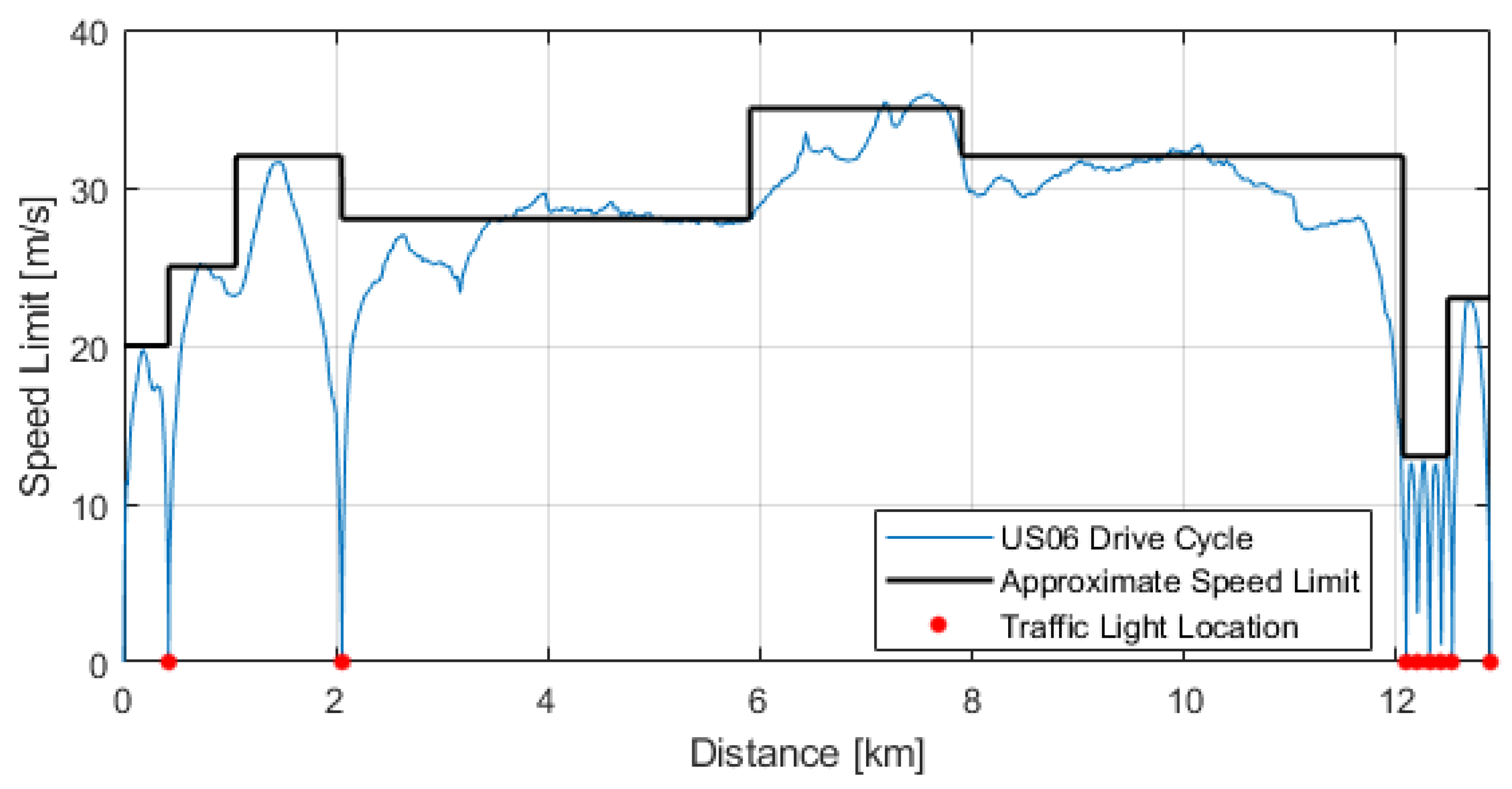
The ANN training data is generated using the optimal speed and SOC trajectories determined using DP over many trips. The speed limits and traffic light positions for the trips were generated using typical drive cycles that captured common driving types, such as highway, urban, and mixed driving. They are based off of five standard drive cycles with some modifications, namely the US06, HWFET, UDDS, NYCC, and LA92 cycles [26]. This ensures that the ANN training data is representative of realistic driving. Each drive cycle was first converted from a speed versus time plot to speed versus distance. The speed limit was approximated by matching the drive cycle with distance coordinates. Traffic lights were placed at locations where the drive cycle slows down to zero or closely approaches zero. Figure 4 shows an example of the speed limits constructed from drive cycles.

The speed profile not only depends on the speed limits and traffic lights but also on surrounding traffic. For each of the drive cycles, five iterations are created where the speed limit is randomized within a certain range to model changes in average traffic flow speed. Traffic light positions remain fixed, but the SPaT is random for each iteration to simulate real-world traffic. The result is a large number of trips defined by speed limits as a function of distance and SPaT. These trips are further divided into road segments of length $N_h$, which are representative of what the vehicle will encounter on the road. For each segment of each trip, DP provides optimal speed and SOC trajectories. The result is a large data set of optimal speed and SOC trajectories over a horizon of length $N_h$. The actual training data set which is fed into the ANN consists of the calculated features shown in Table 1 for each speed and SOC trajectory found by DP.

To obtain the optimal s for each training data entry, a traditional ECMS with a constant s is used. The optimal s is found using the shooting method, where s is varied until the SOC trajectory terminates at the desired final SOC, $SO{C}_f$, starting from an initial SOC, $SO{C}_i$. Therefore, $SO{C}_i$ and $SO{C}_f$ are chosen to be the initial SOC and final SOC for each data entry in the training data. Since the base heuristic is available, matching both the speed and SOC trajectory determined by DP for each horizon will force ECMS to provide charge sustainability without explicitly accounting for the error between the desired final SOC and current SOC. This allows DP-ECMS to take advantage of the entire battery SOC range. Alternative methods which force ECMS to approach the target final SOC after every segment limit the range of SOC and result in more fuel use.

After finding the optimal s for each entry in the data set, the data was split as such: 70% used for training, 15% for validation, and 15% for testing. The ANN was trained using the MATLAB Deep Learning Toolbox [27]. The network contains 2 hidden layers with 25 neurons each and uses the Levenberg–Marquardt method as the training function and a hyperbolic tangent sigmoid transfer function.

2.6. Real-Time Implementation and Synchronization

It is important to note that the objective function for MPC is expressed in distance, while in the supervisory controller, it is in time. Careful choice of horizon length, prediction update rate ($t_c$), and EF update rate ($t_s$) is crucial for real-time implementation. A long horizon window is not practical due to the substantial computational load. Additionally, longer-term predictions are more uncertain due to uncertain future traffic. It was found that the nonlinear MPC with DP as solver can complete one optimization over 600 m in well under 10 s. Hence, the prediction horizon window is set to 600 m, and DP is recalculated every 10 s. For $t_s$, an update rate that is too rapid will react to every minor change and may cause oscillations in the torque demand. On the other hand, updating too slow can cause the adaptation to become unstable and cause SOC to deviate far from the reference value. Based on this reasoning and studies found in the literature [28], $t_s=30$ s is chosen. 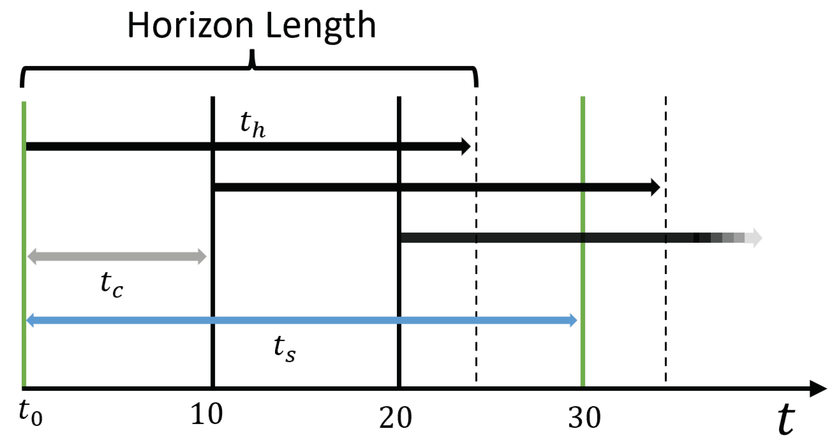Figure 5 shows a timing diagram of the DP-ECMS energy management system. The horizon length is converted to time, $t_h$. This time is not fixed and depends on the horizon length (600 m) and the speed of the vehicle. The horizon length was chosen to be long enough so that $t_c$ will always be much shorter than $t_h$ regardless of the ego vehicle speed. This ensures that the vehicle will never travel further than the horizon length before updating the prediction.

2.7. Baseline FE

To quantify the improvement due to the DP-ECMS solution over a baseline, a human driver model is used based on the well-known intelligent driver model (IDM) [29,30] modified to make the ego vehicle stop at stop signs and traffic lights. This is called the enhanced driver model (EDM) [31] and is expressed by the following equations:

$$\frac{dv}{dt}=\left\{\begin{array}{cc}a\left[1-{\left(\frac{v}{v_0-{\theta }_{offset}}\right)}^{\delta }\right]\hfill & \mathrm{if}v<v_0[\mathrm{Freeway}\mathrm{Driving}]\hfill \\ -b\left[1-{\left(\frac{v_0-{\theta }_{offset}}{v}\right)}^{\delta }\right]\hfill & \mathrm{if}v>v_0[\mathrm{Freeway}\mathrm{Driving}]\hfill \\ a\left[1-{\left(\frac{v}{v_{leader}}\right)}^{\delta }\right]\hfill & \mathrm{if}v<v_{leader}[\mathrm{Car}\mathrm{Following}]\hfill \\ -b\left[1-{\left(\frac{v_{leader}}{v}\right)}^{\delta }\right]\hfill & \mathrm{if}v>v_{leader}[\mathrm{Car}\mathrm{Following}]\hfill \\ -\frac{1}{b}\left(\frac{v^2}{2s}\right)\hfill & \left[\mathrm{Stop}\right]\hfill \end{array}\right.$$

(14)

$$\begin{array}{cc}\hfill s& =x_{leader}-x_{ego}-x_{safe}\hfill \end{array}$$

(15)

$$\begin{array}{cc}\hfill s_{brake}& =\left(1+\frac{c_1}{\delta }\right)\frac{v^2}{2b}\hfill \end{array}$$

(16)

where $v,v_0,\mathrm{and}{v}_{leader}$ are the ego vehicle speed, speed limit, and lead vehicle speed, respectively, a and b are the maximum acceleration and deceleration, respectively, $\delta$ defines driver aggressiveness, ${\theta }_{offset}$ further models driver behavior where a relaxed driver would choose to drive slightly below the speed limit and an aggressive driver will get as close as possible to the speed limit, the term $\left(\frac{c_1}{\delta }\right)$ is a calibration term which captures the dependence of braking distance on aggressiveness, $x_{leader},x_{ego},\mathrm{and}{x}_{safe}$ are the lead, ego, and safe distance, respectively. The safe distance ensures a safe gap to the lead vehicle.

The EDM is used as a benchmark to compare the energy consumption over a trip driven by a human driver to a vehicle driven by the EMS developed in this research. The driver is calibrated to match the aggressiveness of the optimal speed prediction to ensure that the comparison is fair. The term representing the trade-off between fuel consumption and travel time ($\beta$ in Equation (10)) can be thought of as the driver aggressiveness since the vehicle will tend to either drive faster or slower, depending on the value chosen for $\beta$. For the results presented in this research, a value of $\beta =0.65$ is chosen which represents a moderate driver.

The EDM calibration parameters are $[a,b,\delta ,c_1,{\theta }_{offset}]$ and are determined using a genetic algorithm to solve a least squares optimization problem which minimizes the root mean square error:

$$\begin{array}{c}RMS=\sqrt{\frac{1}{N}\sum _{j=1}^N{\left(V_{ED{M}_j}-V_{dat{a}_j}\right)}^2}\end{array}$$

(17)

where N is the number of samples, j is the current sample, $V_{ED{M}_j}$ is the velocity calculated by the EDM and $V_{dat{a}_j}$ is the experimental value. The experimental data used to calibrate the driver model is obtained by running DP, assuming that the vehicle stops at every traffic light along the route. This allows the calibration process to capture acceleration and deceleration to match the behavior of the DP solution.

Table 2. Calibrated EDM parameters.

Parameters	Optimized Values
a [m/s2]	$2.96$
b [m/s2]	$1.54$
$c_1$ [-]	$3.75$
$\delta$ [-]	$1.44$
${\theta }_{offset}$ [m/s2]	$0.82$

shows the optimized parameter values.

The EMS used for the baseline is A-ECMS, where the adaptation is done via PI control based on SOC feedback. The controller adjusts s to minimize the difference between the current SOC and the target SOC with the goal of maintaining charge sustainability. The formulation is as follows:

$$\begin{array}{c}s\left(t\right)=s_0+k_p(x_{ref}-x\left(t\right))+k_I{\int }_0^t(x_{ref}-x\left(\tau \right))d\tau ,\end{array}$$

(18)

where $s_0$ is the EF at $t=0$, $k_p$ and $k_I$ are the proportional and integral gains, respectively, $x\left(t\right)$ is the SOC at time t, and $x_{ref}$ is the reference SOC.

3. Results and Discussion

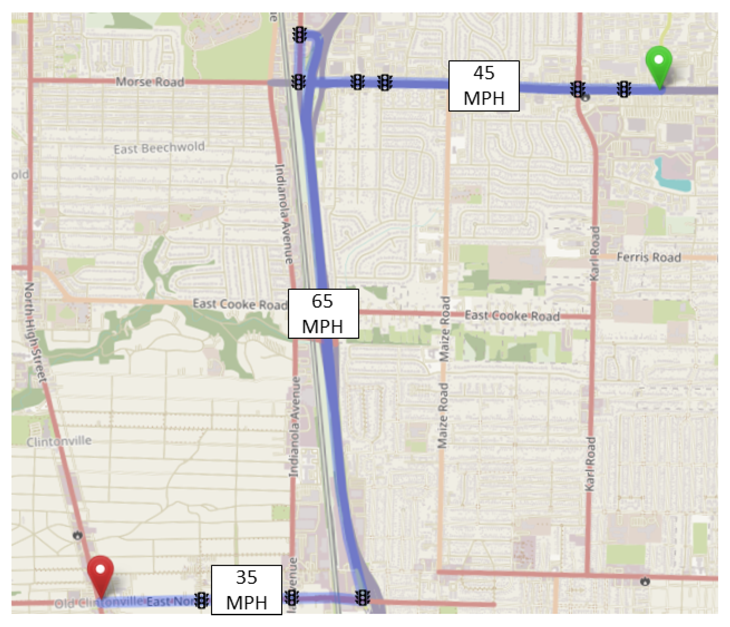
A test route chosen for a simulation study consists of both highway and city driving on local roads in Columbus, Ohio. Figure 6 shows the route on a map along with traffic light locations and speed limits.

Table 3. Route characteristics.

Trip Length	Max. Speed	Avg. Speed	Traffic Lights
8.4 km	30 m/s	23.3 m/s	9

shows relevant route characteristics.

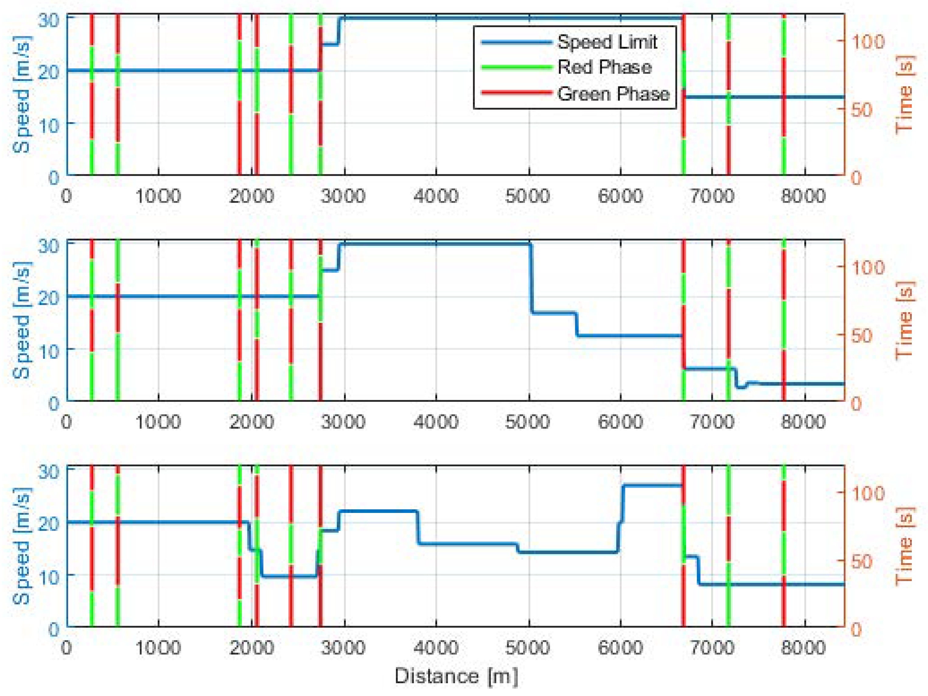
Beginning with the fixed speed limit along the route, traffic patterns typical of daily driving are randomly generated by choosing a random location along the route, a random speed which is less than or equal to the original speed limit, and a random length of speed limit variation. Along the selected route, there are nine traffic lights. A similar approach is used to randomly set the traffic light phase and timing. Examples of randomly generated speed limits over the chosen route are shown in Figure 7, where colored (green or red) vertical lines indicate the traffic light location and the phase the light is in. The size of each vertical colored segment indicates how long the phase lasts.

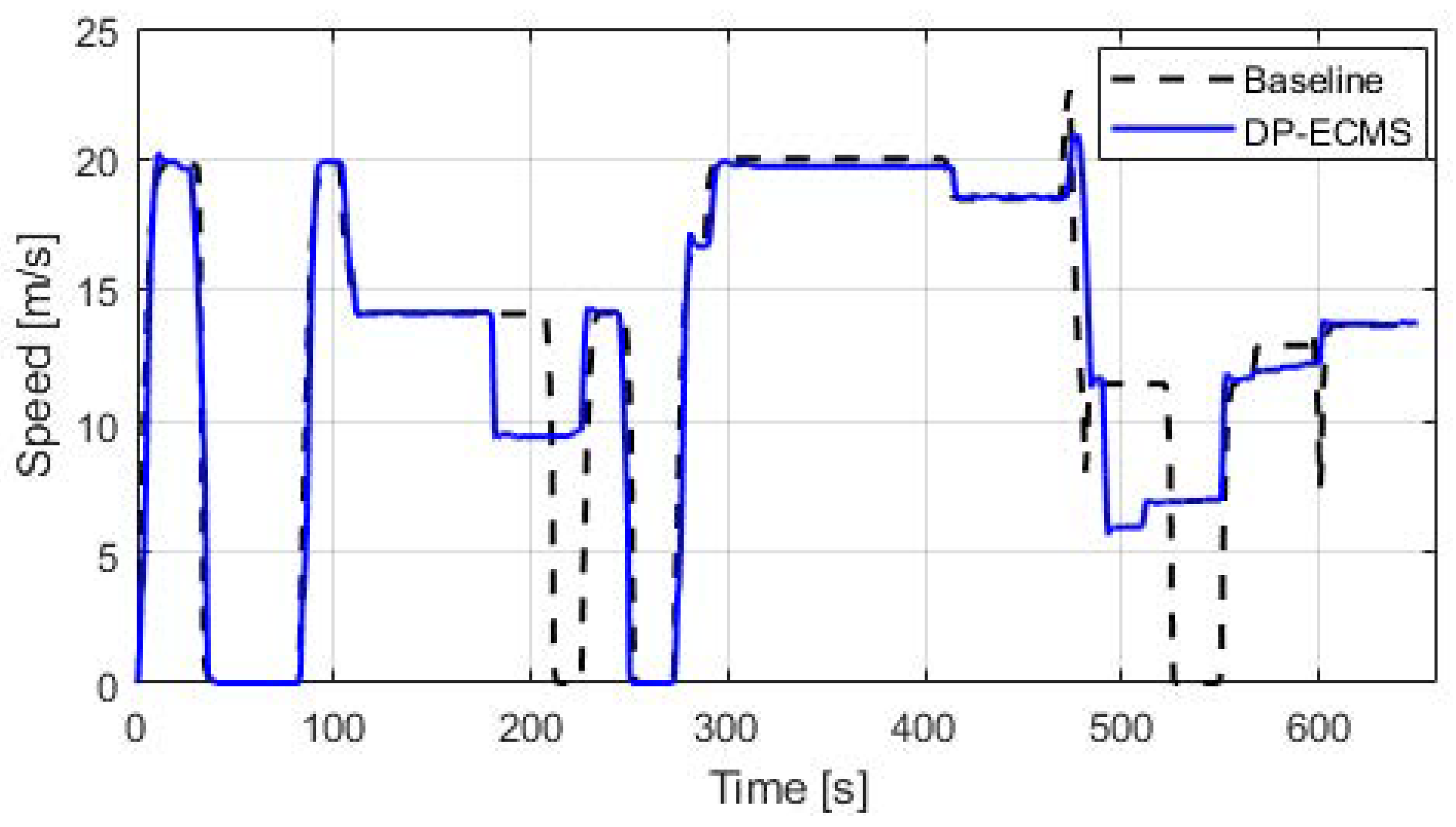
The ability of the MPC to avoid red lights and the corresponding FE benefit from the EMS is shown first, followed by the FE distribution over several randomly generated traffic and SPaT patterns.

Figure 8 shows the speed profiles for both DP-ECMS and the baseline for one trip. When the vehicle is approaching an intersection during its red phase, the baseline driver initiates the stop sequence in anticipation of the red light. Since it has no knowledge of the signal timing, there is no way to determine if the light will turn green before the vehicle reaches the intersection. DP-ECMS is able to use available look-ahead data to calculate the appropriate speed to arrive at the light on green and adjusts accordingly. For all simulations, the DSRC range is assumed to be 500 m based on studies found in the literature [11,32,33]. 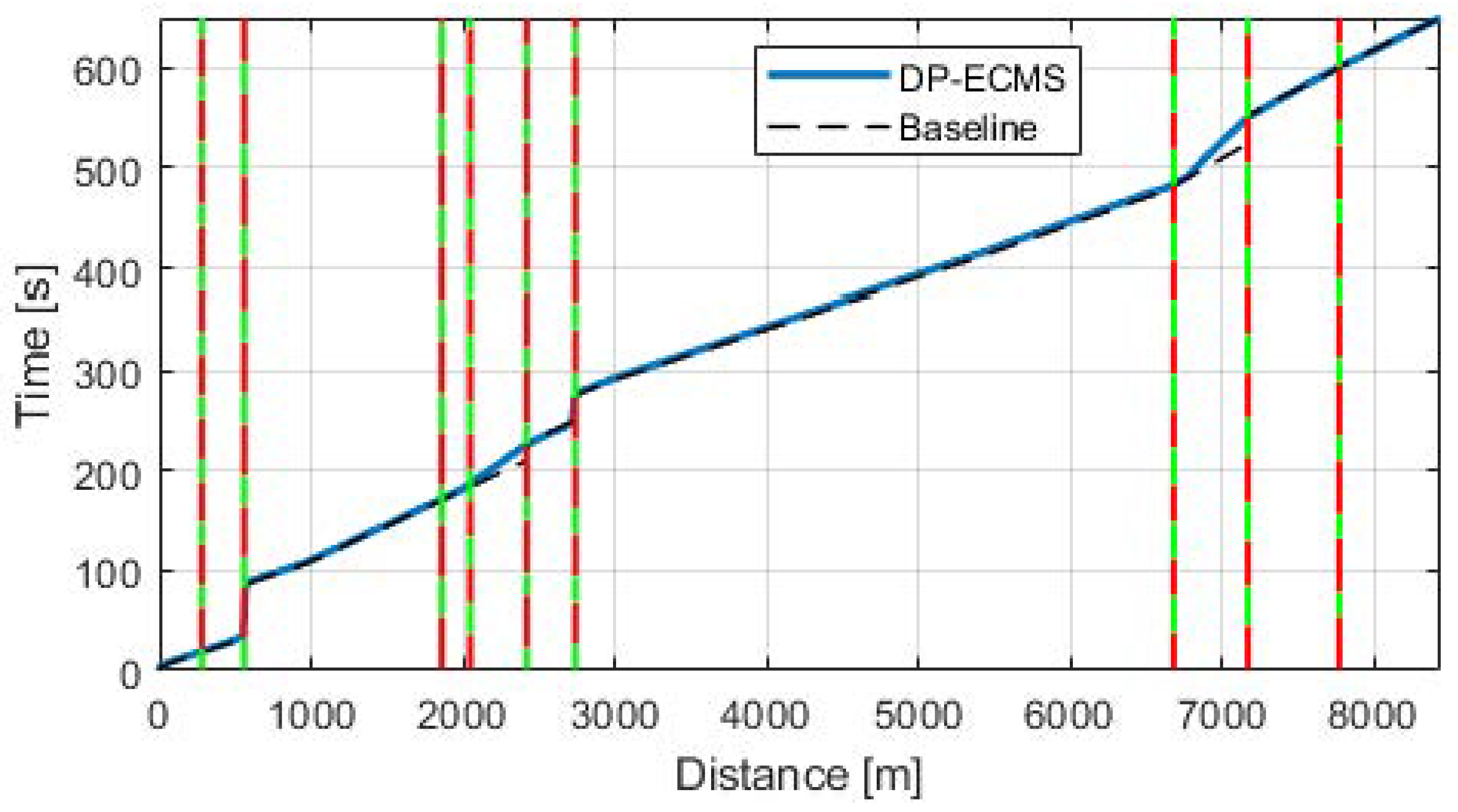Figure 9 shows the travel time versus the distance traveled. DP-ECMS slows the vehicle down just enough to pass through the green window when possible, while the baseline will always initiate a stop if the light is red. The travel time is approximately equal for both methods.

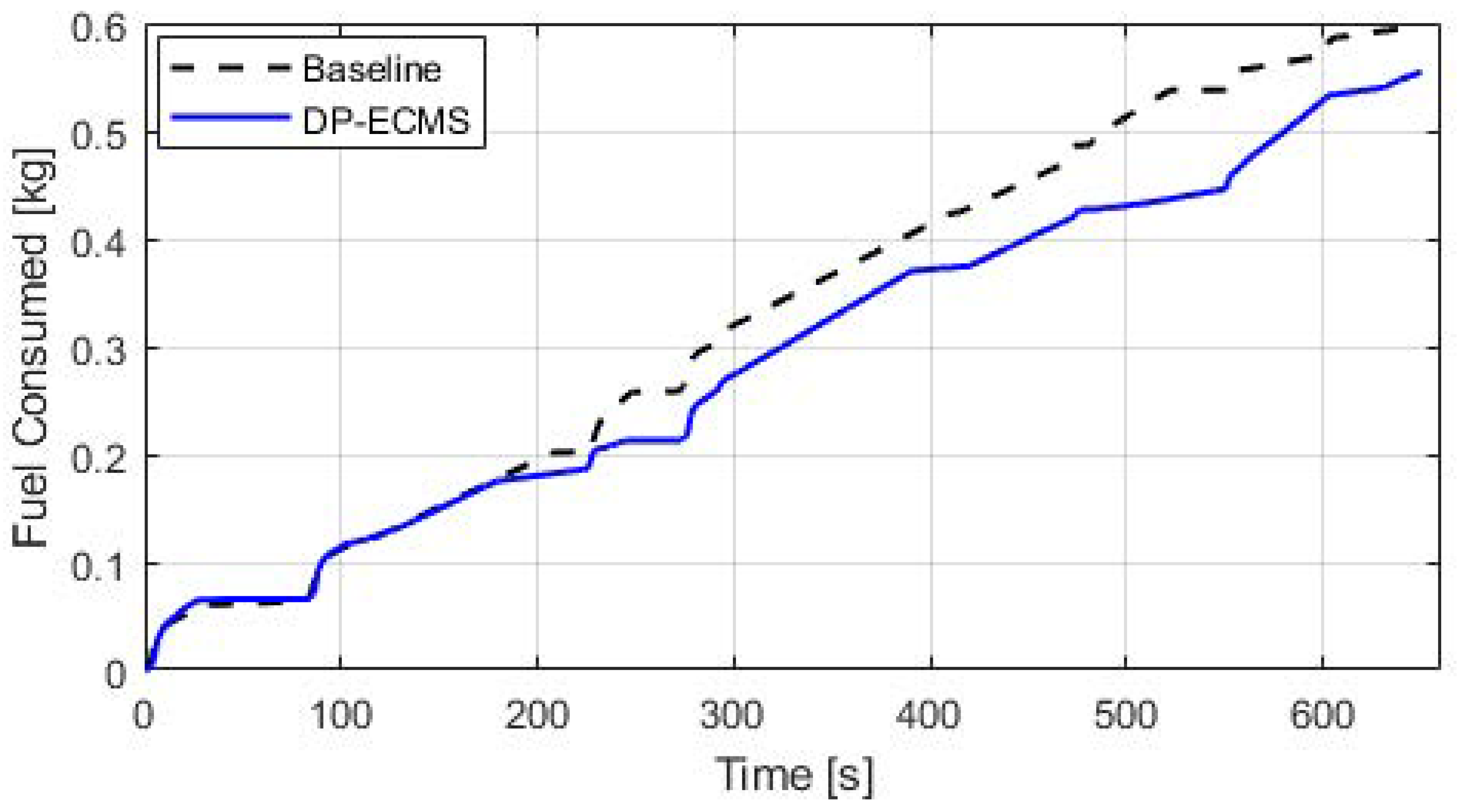
Figure 10 compares the fuel consumption for the two systems. DP-ECMS achieves a 7.1% reduction in fuel consumed compared to the baseline. The use of DP over the full route, assuming prior knowledge of the vehicle instantaneous speed for the entire trip, provides an ideal fuel consumption. When compared to this DP solution (0.53 kg total fuel consumed), the baseline consumes 13% more fuel than DP (0.59 kg total fuel) and the proposed method uses 5% more fuel (0.56 kg total fuel) than DP. 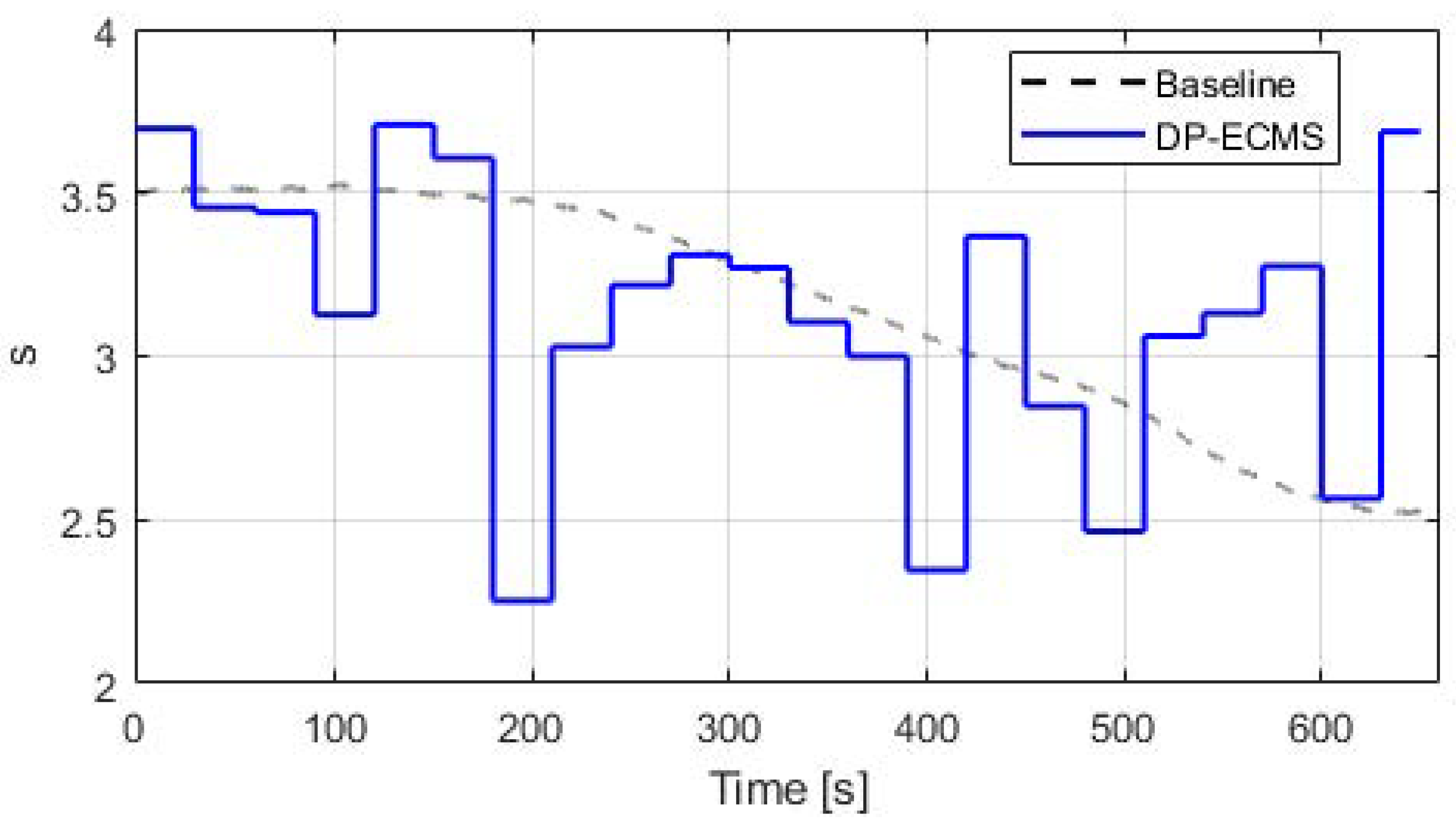It is also shown in Figure 11 that both strategies are approximately charge-sustaining, and the corresponding adapted EFs are shown in Figure 12. Although tailpipe emissions are not directly considered in the objective function, reducing the number of traffic light stops provides the added benefit of emissions reduction [34]. Therefore, it is expected that the proposed EMS will reduce emissions along with fuel consumption. A direct way of addressing tailpipe emissions is to incorporate the emissions in the cost function and after-treatment system dynamics in the dynamic constraints [35].

A Monte Carlo analysis is conducted with a sample size of 85, where the random variables are SPaT and average traffic speed. Both the baseline and DP-ECMS are run using the same traffic and SPaT patterns to ensure that the results are directly comparable. Considering that the vehicle in question has an electrified powertrain, it is important to keep track of the battery SOC. A common way to account for differences in the final and initial SOC is to apply a correction factor to fuel consumption based on the magnitude of the deviation [36]. However, this process can be imprecise and is difficult to properly apply to a large number of samples. To simplify the process, each trip was repeated 10 times and the FE (MPG) was computed for the duration of the 10 cycles. By doing so, the small deviations in the SOC are negligible over the energy consumed by burning fuel over 10 trips. 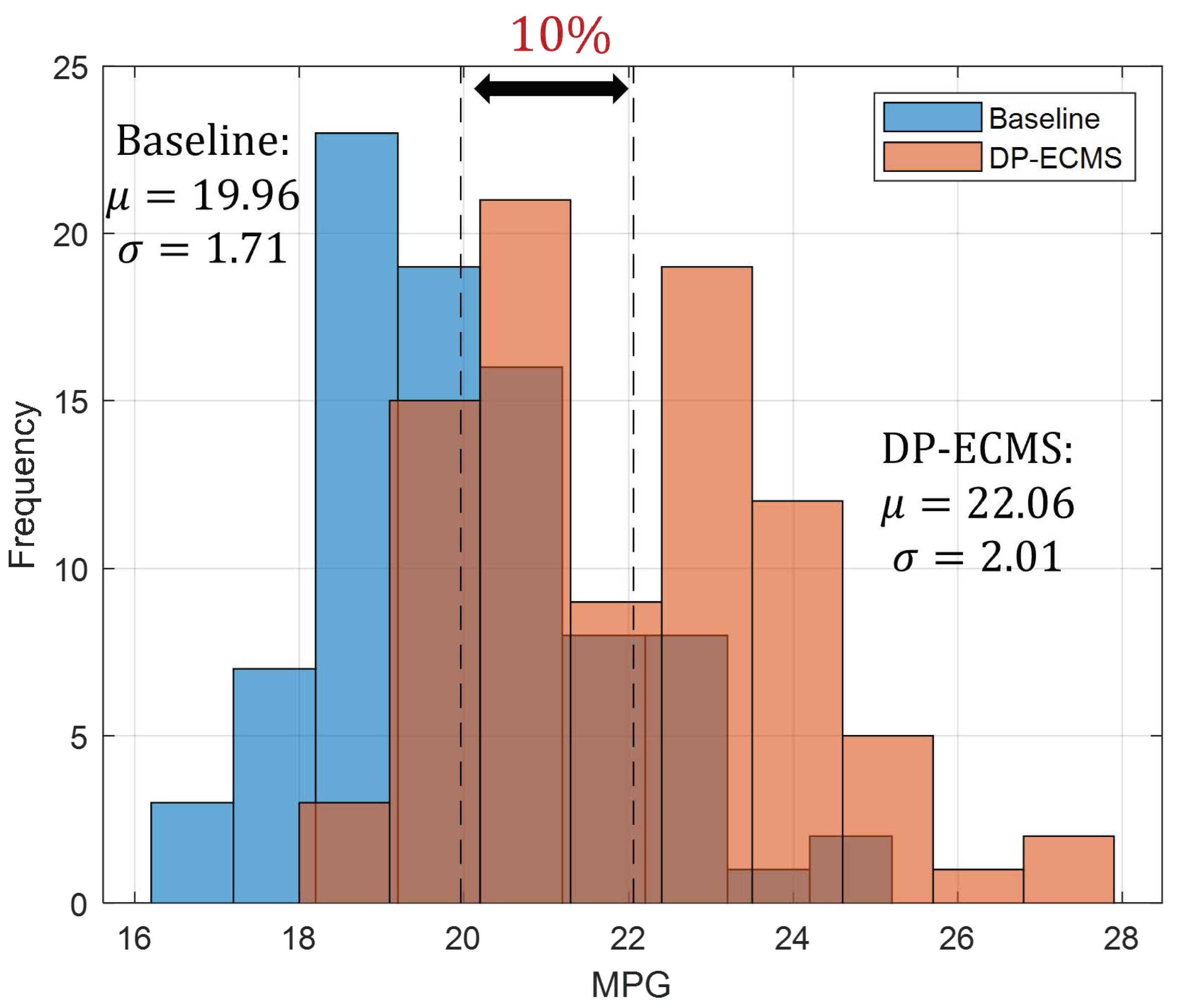Figure 13 shows the Monte Carlo simulation results with overlaid histograms for both DP-ECMS and the baseline along with the mean and standard deviation.

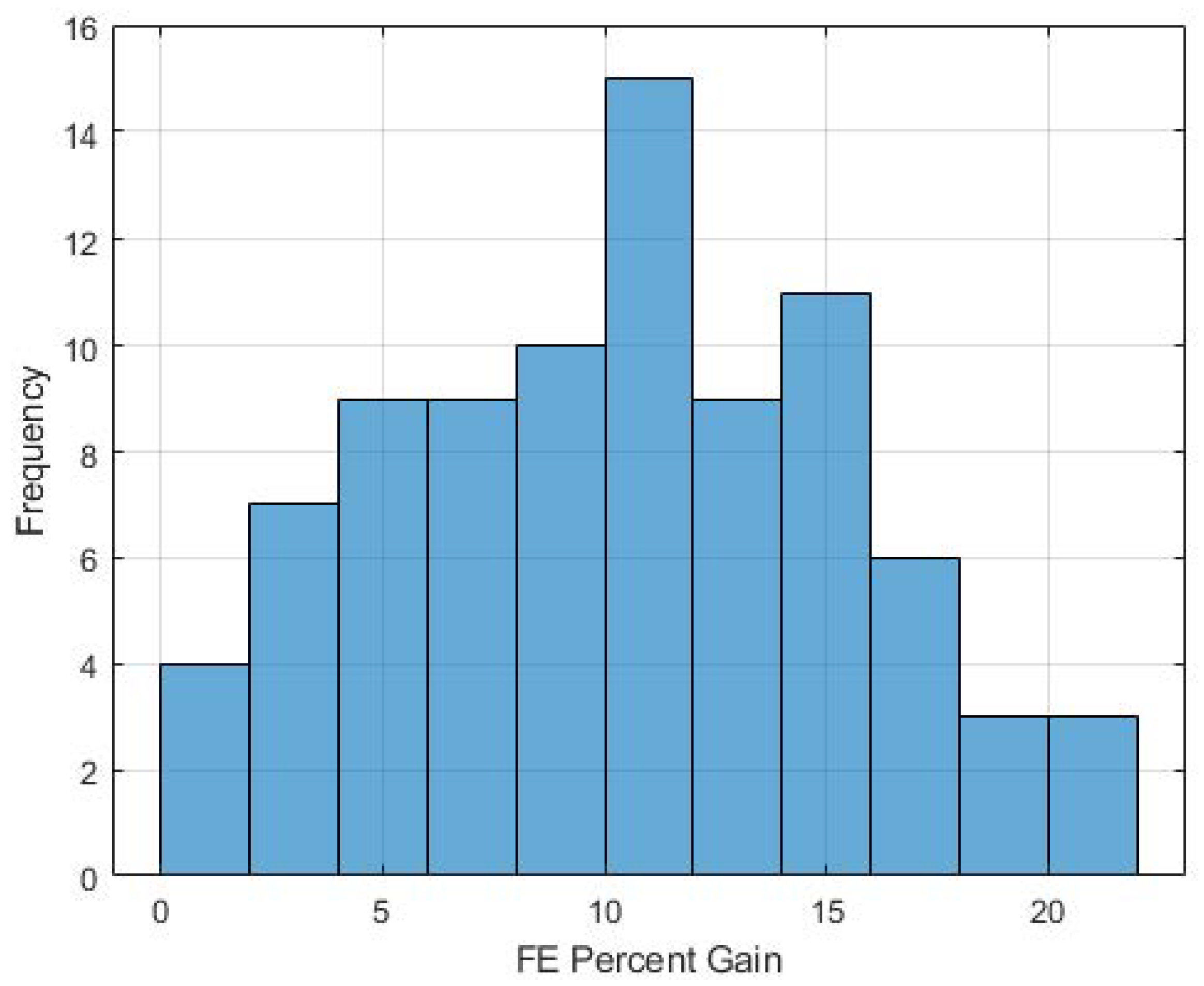
The DP-ECMS method yields MPG values which range from about 18 to 28 MPG, while the baseline ranges from 16.1 to 25 MPG. The median bin for the baseline is 18.2 to 19.2 MPG, whereas for DP-ECMS, it is 20.2 to 21.3 MPG. DP-ECMS yields an average FE of 22.06 MPG, while the baseline is 19.96 MPG. The results show that, on average, the DP-ECMS provided a 10% FE increase over baseline. A histogram of the percent gain in FE is shown in Figure 14, which shows gains in FE for each trip.

By plotting the percent gain, it can be seen that the algorithm always performs either the same as or better than the baseline. It is expected that there will be cases where DP-ECMS will have similar FE to the baseline. Since the biggest advantage of DP-ECMS is the use of look-ahead data, if there are cases where there is no traffic and all green lights, there will most likely not be much benefit to having look-ahead data. Likewise, if the traffic is so heavy that the vehicle is not able to leverage the future knowledge, it will behave similar to the baseline.

4. Conclusions

This paper presented a novel approach for integrated EMS and speed control using A-ECMS considering look-ahead data. A data-driven approach using ANN was developed to predict the optimal EF for ECMS. A unique combination of a DP-based optimal control solution for speed profiling and ECMS with an optimal EF predictor was shown to be capable of online implementation on vehicle hardware. It was shown that a simple rule-based approach to handling the traffic light signal phase and timing avoids unnecessary stops at red lights and consequently reduces fuel consumption. A receding horizon optimal control framework was used to adapt to disturbances along the route and predict the future speed and SOC trajectories. A data-driven EF adaptation approach was shown to be beneficial, since the neural network is able to learn the nonlinear relationship between the input features extracted from optimal future trajectories and the corresponding optimal EF. This further allows ECMS to compute the optimal torque split ratio for each future horizon as opposed to simply reacting to the information available at each instant. A statistical analysis showed that DP-ECMS always performs equal to or better than the baseline, and an average 10% FE improvement was achieved while maintaining an approximately equal travel time. The steps towards implementing the proposed methods on vehicles should include various levels of x-in-the-loop testing, I/O considerations like CAN delay, errors and synchronization, and optimization of the code for the target hardware.