Cardiac Magnetic Resonance Left Ventricle Segmentation and Function Evaluation Using a Trained Deep-Learning Model

Abstract

Cardiac MRI is the gold standard for evaluating left ventricular myocardial mass (LVMM), end-systolic volume (LVESV), end-diastolic volume (LVEDV), stroke volume (LVSV), and ejection fraction (LVEF). Deep convolutional neural networks (CNNs) can provide automatic segmentation of LV myocardium (LVF) and blood cavity (LVC) and quantification of LV function; however, the performance is typically degraded when applied to new datasets. A 2D U-net with Monte-Carlo dropout was trained on 45 cine MR images and the model was used to segment 10 subjects from the ACDC dataset. The initial segmentations were post-processed using a continuous kernel-cut method. The refined segmentations were employed to update the trained model. This procedure was iterated several times and the final updated U-net model was used to segment the remaining 90 ACDC subjects. Algorithm and manual segmentations were compared using Dice coefficient (DSC) and average surface distance in a symmetric manner (ASSD). The relationships between algorithm and manual LV indices were evaluated using Pearson correlation coefficient (r), Bland-Altman analyses, and paired t-tests. Direct application of the pre-trained model yielded DSC of 0.74 ± 0.12 for LVM and 0.87 ± 0.12 for LVC. After fine-tuning, DSC was 0.81 ± 0.09 for LVM and 0.90 ± 0.09 for LVC. Algorithm LV function measurements were strongly correlated with manual analyses (r = 0.86–0.99, p < 0.0001) with minimal biases of −8.8 g for LVMM, −0.9 mL for LVEDV, −0.2 mL for LVESV, −0.7 mL for LVSV, and −0.6% for LVEF. The procedure required ∼12 min for fine-tuning and approximately 1 s to contour a new image on a Linux (Ubuntu 14.02) desktop (Inter(R) CPU i7-7770, 4.2 GHz, 16 GB RAM) with a GPU (GeForce, GTX TITAN X, 12 GB Memory). This approach provides a way to incorporate a trained CNN to segment and quantify previously unseen cardiac MR datasets without needing manual annotation of the unseen datasets.

1. Introduction

Quantification of left ventricular (LV) function is crucial for risk stratification, diagnosis, and treatment of cardiac disease [1]. Cardiac magnetic resonance imaging (MRI) has been established as the gold standard for evaluating left ventricular function [2], including LV myocardial mass (LVMM), end-diastolic volume (LVEDV), end-systolic volume (LVESV), stroke volume (LVSV), and ejection fraction (LVEF). To generate these measurements, segmentation of the LV structures is required as a first step. Manual segmentation of cardiac MRI requires intensive efforts from users, depends on the experience of observers, introduces user variability, and is not compatible with efficient and high throughput cardiac imaging workflow [3].

Various methods have been developed for cardiac MR image analysis and demonstrated utility for use in research and clinical settings. Non-learning based methods [4,5] heavily rely on hand-crafted features with limited representation capability and generally provide suboptimal performance [6]. Recently, the development and use of deep convolutional neural networks (CNN) has achieved remarkable success for numerous cardiac imaging tasks [7]. With the availability of large annotated datasets and powerful computational platforms, these learning-based methods can automatically learn highly discriminative features through feature abstraction in a hierarchical manner. Recent studies [3,8,9] showed significant promise of using neural networks for heart segmentation in cardiac cine MRI, as recently reviewed [10]. Although promising, these studies mainly trained and tested CNNs on datasets acquired using the same scanner or at the same healthcare center, which represents a limited number of applications of deep learning in most research and clinical settings. Unfortunately, these [3,8] and other investigations [11] also demonstrated that deep-learning models trained on one domain (source) do not generalize well to a new domain (target) and direct application of a pre-trained model to a new dataset often yields degraded performance because of the well-known domain shift issue facing the community.

To facilitate translation of this important tool for widespread use in research and clinical care, it is urgently required to improve the generalizability of deep-learning methods to datasets collected using different imaging settings on different systems at various locations in patients with distinct diseases. Domain adaptation [12] aims to address this issue by fine-tuning a pre-trained model using a small amount of labeled data from a target domain, or by learning domain-invariant features or transforming data from the target domain to resemble the source domain. For example, previous studies [8,13] fine-tuned a pre-trained model using manually annotated datasets for new cardiac MRI segmentation tasks in a supervised manner. Other studies employed adversarial learning to transform data in a one domain (source) to resemble data in another domain (target) at the image level [14] or image-and-feature level [15] for unsupervised domain-adaptation-based cardiac image segmentation. Data augmentation [16] represents a very different approach to solving this problem by artificially enlarging the training datasets through extensive transformations to train a model that is robust to potential variations in new domains. Although commonly used classical data augmentation techniques (e.g., geometrical transformation, noise, contrast and blurring perturbation, histogram equalization and matching) have been widely used in various applications, other advanced and extensive augmentation techniques have also demonstrated effectiveness in addressing the domain shift issue [17,18]. In particular, recent studies using advanced data augmentation techniques demonstrated higher performance than several adversarial learning-based domain-adaptation methods for several medical image segmentation tasks [17,18].

Although the previous studies demonstrated some promise in tackling the domain shift issue for medical image segmentation, these algorithms have limitations. For example, domain adaptation using labeled data from a target domain requires a substantial amount of time and expertise for manual annotation and is not compatible with efficient research and clinical workflow. Adversarial learning that transforms a dataset from a source domain to resemble a target domain typically requires a large dataset from the target domain and a long time for re-training/fine-tuning. Data augmentation aims to learn non-domain specific features by performing extensive transformations to change the appearance of training datasets and often generates non-realistic datasets that do not resemble real world cases, which may or may not adversely affect the performance. Another potential issue associated with these techniques is the increased difficulty of algorithm interpretability because of the “black box” nature of deep-learning methods. Here, we proposed a different approach to tackling the domain shift issue. In particular, we employed a machine-learning method to automatically segment a subset of an unseen dataset without manual annotations to fine-tune a pre-trained deep-learning model to segment cardiac MRI datasets from a different domain. The proposed approach required 12 min to segment a relatively small dataset of 10 subjects for fine-tuning and to update the pre-trained model without affecting algorithm interpretability. Importantly, our approach yielded several commonly used and clinically relevant LV function measurements that are in strong agreement with expert manual analyses; this was not demonstrated in the previous studies. A preliminary version of this work has been published in conference proceedings [19] and there are substantial differences between the current work and the previous version [19]. In the current version, we reviewed some commonly used techniques (e.g., domain adaptation and data augmentation) that are developed to tackle the domain shift issue and discussed the advantages/limitations of these techniques. We also provided some details regarding the mathematical formulation and upper bound-based iterative optimization of the proposed continuous kernel-cut method. In addition, we implemented several state-of-the-art deep-learning segmentation models (DeepLabV3+ and an optimized style-intensity augmentation method) and performed comprehensive comparison between these methods and our approach. Furthermore, we discussed the study limitations and proposed some future work directions. These elements were not included in our previous work [19] and represents some of the major differences in the current work.

2. Methods

2.1. Cardiac MRI Datasets

We investigated two cine cardiac MR datasets from the Left Ventricle Segmentation Challenge (LVSC) held in 2009 [20] and the 2017 Automated Cardiac Diagnosis Challenge (ACDC) [9]. The LVSC dataset (https://www.cardiacatlas.org/studies/sunnybrook-cardiac-data/, accessed 20 March 2021) consists of 45 subjects (mean age = 61 ± 15 years, age range = [23, 88] years; 32 male) enrolled in clinical studies at Sunnybrook Health Sciences Centre (Canada), including healthy volunteers (n = 9) and patients with hypertrophy (n = 12), or with heart failure with (n = 12) and without (n = 12) infarction. Two-dimensional short-axis cine images of the whole heart were obtained with as SSFP sequence (voxel size = 1.25–1.56 mm${}^2$, slice thickness = 8–10 mm, inter-slice gap = 8 mm, 6–12 slices, 20 phases per cardiac cycle) on a 1.5T scanner (Signa, GE Healthcare, Milwaukee, WI, USA). For each subject, both the myocardium (LVM) and blood cavity (LVC) of the left ventricle in the cine images at the end-diastole were manually segmented by a cardiologist, and only the LV cavity was manually segmented at the end-systolic phase. Therefore, only the cine MRI datasets at the end-diastolic phase (n = 45 images) were used in this study.

The ACDC dataset (https://www.creatis.insa-lyon.fr/Challenge/acdc/, accessed 20 March 2021) comprises 100 participants (mean weight = 75 ± 17 kg; mean height = 171 ± 10 cm) acquired in clinical routine at the University Hospital of Dijon (France). The dataset covers five categories of well-defined pathologies (n = 20 subjects in each category): heart failure with myocardial infarction, dilated cardiomyopathy, hypertrophic cardiomyopathy, and abnormal right ventricle, as well as healthy subjects. Two-dimensional short-axis cine images covering the entire LV were acquired on 1.5T or 3.0T scanners (Siemens Aera and Siemens Trio, Siemens Medical Solutions, Germany) using an SSFP sequence (voxel size = 1.34–1.68 mm${}^2$, slice thickness = 5–10 mm, inter-slice gap = 5 mm (sometimes), 6–18 slices, 28–40 phases per cardiac cycle). The dataset had substantial variability in image quality, including noise, motion and banding artefacts, MR low-frequency intensity fluctuation, and varying field-of-view. Manual segmentation of the LVM and LVC was performed on the cine images at both end-diastolic and end-systolic phases, which were double-checked by two independent experts to reach consensus.

We note that the manual segmentation of the LVSC dataset is not very consistent between subjects and there is substantial “noise” in manual annotations. In addition, the LVSC dataset contains cine images with LV cavity and myocardium segmentation only at the end-diastolic phase. We used the LVSC dataset for CNN pre-training, which provides additional opportunity to explore the tolerance to annotation noise and generalizability from end-diastolic phase to end-systolic phase for a deep-learning segmentation algorithm. The ACDC dataset was randomly divided into 10 and 90 subjects for CNN fine-tuning and testing, respectively. All data used in this study were anonymized and ethics approval for using these public datasets was exempted.

2.2. Algorithm Workflow

We used a 2D U-net [21] that comprised a symmetric contracting and expanding path with five levels. Each level consists of two blocks of 3 × 3 convolution and a rectified linear unit, followed by max-pooling in the contracting path or up-sampling in the expanding path; the number of feature maps was 16 in the top level and increased to 256 in the bottom level. The network was pre-trained on 45 images from the LVSC dataset for 200 epochs by minimizing the cross-entropy between model prediction and manual reference segmentation using an ADAM optimizer (learning rate = 10${}^{-4}$). Spatial data augmentation, including translation (−50–50 pixels), random rotation (−50–50${}^{\circ }$), voxel size and intensity scaling (0.75–1.25 times), and elastic deformation, was performed in parallel. To further minimize overfitting and improve CNN segmentation generalizability, Monte-Carlo dropout [22] (MCD, dropout rate = 0.5) was applied to each block in the bottom three levels of the 2D U-net. These settings were adopted for the following fine-tuning procedure.

Figure 1 provides the schematic of our proposed algorithm. Briefly, the trained U-net was applied to the 10 ACDC fine-tuning subjects. For each subject, test-time MCD was applied to generate 50 segmentation samples ($s_1\left(x\right),s_2\left(x\right),\dots ,s_{50}\left(x\right)$, $x\in \mathrm{\Omega }$); the mean of the associated probability maps were calculated to derive the “mean” segmentation $\overline{s}\left(x\right)$. In addition, the standard deviation of the 50 segmentation samples was calculated for each pixel and used as pixel-wise U-net segmentation uncertainty $\omega \left(x\right)$, i.e., $\omega \left(x\right)\propto \frac{1}{std\left(\right\{s1\left(x\right),s2\left(x\right)\dots ,s50\left(x\right)\left\}\right)}$, $x\in \mathrm{\Omega }$. The derived “mean" segmentation $\overline{s}\left(x\right)$ was post-processed using a recently developed continuous kernel-cut (CKC) segmentation method, which demonstrated effectiveness in post-processing cardiac MRI CNN segmentation outputs [3,23,24]. The CKC segmentation algorithm employs normalized cut for balanced pair-wise feature clustering and continuous regularization on image grids to generate spatially smooth contours. In addition, we proposed to use the derived CNN “mean” segmentation as descent initialization of the CKC algorithm such that in regions with high U-net segmentation uncertainty (i.e., $\omega \left(x\right)$ is relatively low), the final segmentation $u\left(x\right)$ can be more different from the “mean” segmentation $\overline{s}\left(x\right)$ and vice versa. To this end, we derived the deep-learning uncertainty-guided CKC segmentation algorithm by minimizing the following function:

$$\sum _{l\in L}-\frac{u_l^{T}X{u}_l}{\mathbf{1}X{u}_l}+{\int }_{\mathsf{\Omega }}g\left(x\right)\left|\nabla u_l\left(x\right)\right|dx+{\int }_{\mathsf{\Omega }}\omega \left(x\right)·\left|u_l\left(x\right)-\overline{s_l}\left(x\right)\right|dx,u_l\in \{0,1\},$$

(1)

subject to ${\sum }_{l\in L}{u}_l\left(x\right)=1$, $\forall x\in \mathrm{\Omega }$. In Equation (1), $u_l\left(x\right)\in \{0,1\}$ is decomposed from the final segmentation $u\left(x\right)$ and indicates if voxel x is in region $l\in L=\{LVM,LVC,background\}$, X is a matrix where each element $X(i,j)$ indicates if voxel j is within the K-nearest neighbor of voxel i, 1 is an all-ones matrix, $g\left(x\right)$ is a boundary weight function based on image contrast edges, and $\omega \left(x\right)$ enforces the similarity of CNN initial segmentation $\overline{s_l}\left(x\right)$ and CKC final segmentation $u_l\left(x\right)$ for each region l. Of note, $\overline{s_l}$ was decomposed from $\overline{s_l}$ similar to $u_l\left(x\right)$. The CKC algorithm in Equation (1) integrates the advantages of balanced portioning of image features in high-dimensional space and spatially smooth segmentation that mimics the behavior of manual delineation [3,24,25].

Direct optimization of the high-order and non-smooth function in Equation (1) is particularly challenging. Following the previous work [3,23,26], we adopted an upper bound optimization technique to simplify the optimization of Equation (1) by deriving and optimizing a series of upper bound functions of Equation (1), assuming that the upper bound function is easier to minimize than the original formulations. Briefly, for any given segmentation ${\widehat{u}}_l$, $l\in L$, $x\in \mathrm{\Omega }$, previous studies [26] showed that the following is an upper bound function of Equation (1):

$$\sum _{l\in L}〈\frac{X\mathbf{1}{\widehat{u}}_l^{T}X{\widehat{u}}_l}{{\left(1X{\widehat{u}}_l\right)}^2}-\frac{2X{\widehat{u}}_l}{\mathbf{1}X{\widehat{u}}_l},u_l〉+{\int }_{\mathsf{\Omega }}g\left(x\right)\left|\nabla u_l\left(x\right)\right|dx+{\int }_{\mathrm{\Omega }}\omega \left(x\right)·\left|u_l\left(x\right)-\overline{s_l}\left(x\right)\right|dx,u_l\in \{0,1\},$$

(2)

where $〈,〉$ and ${}^T$ denote inner product and transpose, respectively; the first term in Equation (2) is linear with respect to $u_l$ that we aim to solve. Through convex relaxation, i.e., by relaxing $u_l\in \{0,1\}$ to $u_l\in [0,1]$, we can derive a convex relaxed formulation of Equation (2), which can be efficiently and globally optimized using a continuous min-cut/max-flow algorithm on a graphics card [27,28]. We refer readers to the previous studies [27,28] for the details of the continuous min-cut/max-flow algorithm. Please note that Equation (1) was optimized iteratively; for each iteration, we derived an upper bound using Equation (2) and minimized the upper bound to generate a solution ${\widehat{u}}_l$, which was used to update the upper bound for the next iteration. In particular, for the first iteration we used the derived CNN “mean” segmentation ${\overline{s}}_l$l as the given solution ${\widehat{u}}_l$. This process was iterated several times until convergence (we observed convergence typically within five iterations in this study) to derive the final solution to Equation (1). We refer readers to previous studies [3,24] for the details of minimizing the CKC segmentation model in Equation (1). Upon CKC algorithm convergence, the final segmentation of the fine-tuning dataset (without manual labels) was saved and used to update the trained U-net model for another 20 epochs in ∼10 min. This procedure was iterated until convergence and the final U-net model was tested on the remaining 90 ACDC subjects for LV indices quantification. We also implemented several commonly used methods for comparison, including:

• A naive method (Naive): The trained U-net was used to segment the 90 ACDC test subjects directly.
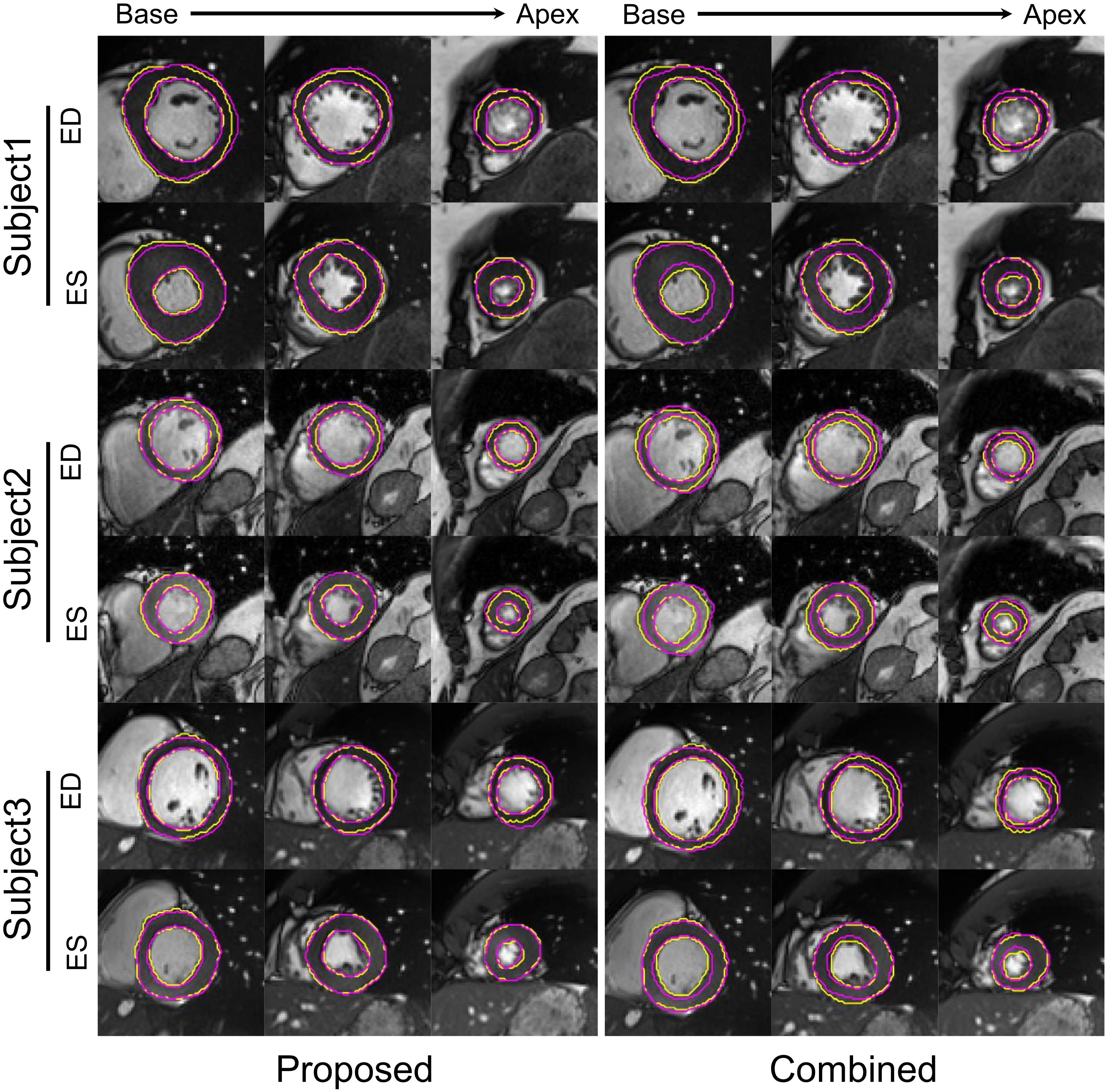
• A combined method (Combined) that integrated MCD, spatial augmentation, and style-intensity augmentation method. We explored the effects of MCD, spatial augmentation, and advanced style-intensity augmentation for U-net training; the optimal combination of the three components constitutes the combined method. A recent study [17] proposed style-intensity augmentation during network training to tackle the domain shift issue and demonstrated state-of-the-art performance in breast segmentation in MRI datasets from a different domain. Style-intensity augmentation comprises style transfer and intensity remapping, which produce non-realistic looking MR scans while preserving the image shapes. The style transfer procedure uses features extracted from style images to augment the training images, randomizing the color, texture and contrast but preserving the geometry [29]. The intensity remapping technique generates a random mapping function to map the original image signal intensities to new values. This method is based on the assumption that by considerably changing the appearance of training images, the network will focus on non-domain specific features, e.g., the geometric shape of breast that is preserved in different breast MR datasets [17]. The optimized combined method was applied to the ACDC test dataset.
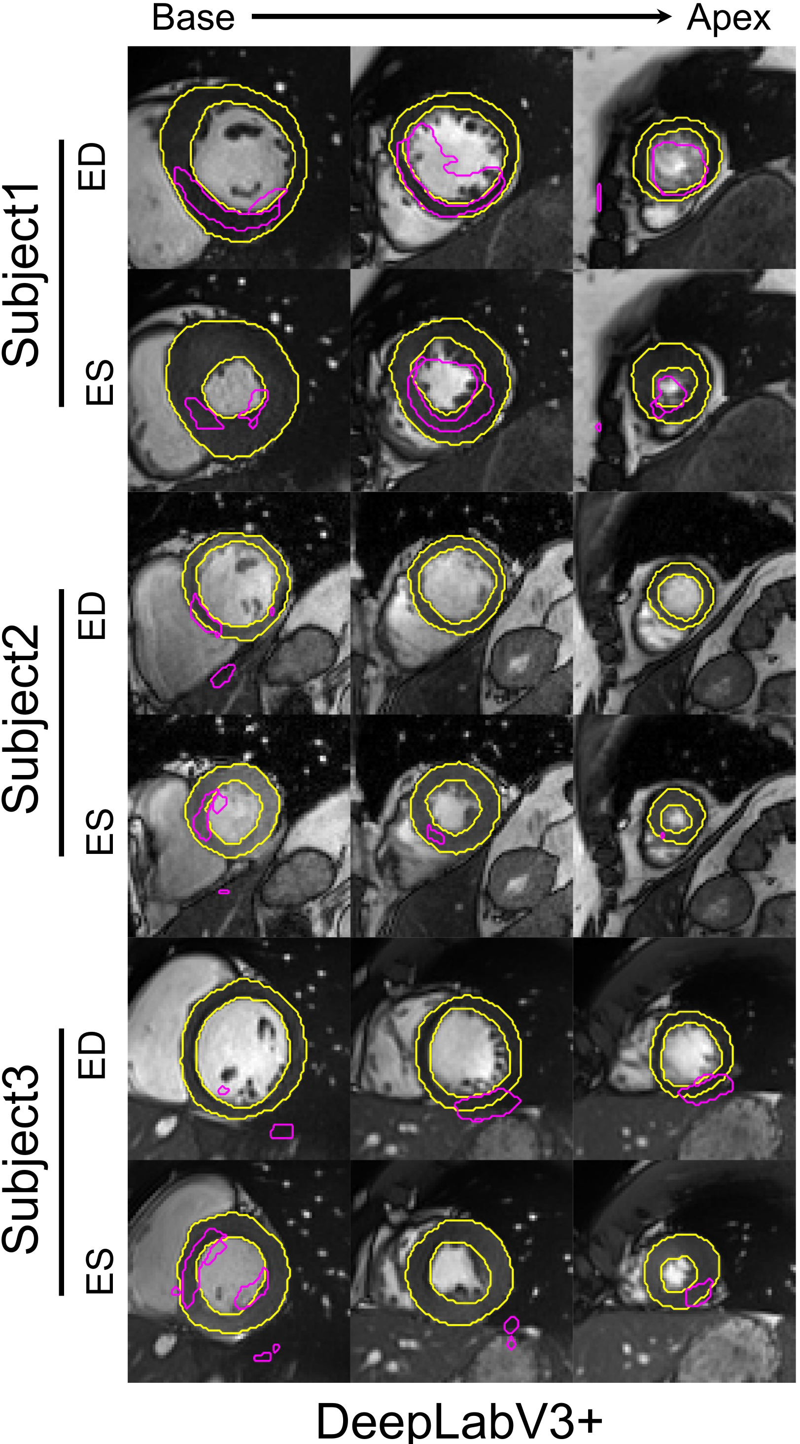
• DeepLab: DeepLabV3+ [30], a top performing neural network in several medical image segmentation challenges, was trained on the LVSC dataset and tested on the ACDC test dataset.

Of note, the proposed algorithm and the naive method were implemented based on the same settings, i.e., MCD+spatial augmentation, and the proposed algorithm incorporated the fine-tuning procedure. The proposed algorithm, the naive and the combined methods were implemented using TensorFlow 1.4.0; DeepLabV3+ was implemented with Keras 2.2.4. All were run on Python 2.7.14 platforms on a GPU (Tesla P100, NVIDIA Corp., Santa Clara, CA, USA). The CKC segmentation algorithm was implemented using MATLAB 2013a (MathWorks, Natick, MA, USA) and CUDA (CUDA v8.0, NVIDIA Corp., Santa Clara, CA, USA) on a Ubuntu 14.02 desktop with a GPU (GeForce, GTX TITAN X, Santa Clara, CA, USA).

2.3. Evaluation Methods

Algorithm performance was evaluated for LV segmentation and function measurements. LV segmentation accuracy was evaluated using Dice coefficient (DSC) and average surface distance in a symmetric manner (ASSD) by comparing algorithm and manual segmentation masks [24,31]. We denote $R_a$ and $R_m$ the algorithm and manual segmentation, respectively. DSC measures the overlap of $R_a$ and $R_m$ and is calculated as: $\frac{2\left|R_a\cap R_m\right|}{\left|R_a\right|+\left|R_m\right|}$, where $\left|.\right|$ represents the size of a mask. ASSD evaluates the closeness between the algorithm and manual segmentation boundaries and is given as: $\frac{1}{2}\{\frac{1}{\left|\partial R_a\right|}{\sum }_{p\in \partial R_a}d(p,\partial R_m)+\frac{1}{\left|\partial R_m\right|}{\sum }_{p\in \partial R_m}d(p,\partial R_a)\}$, where $\partial R_a$ represents the algorithm segmentation boundary and $d(p,\partial R_a)$ is the shortest Euclidean distance from a vertex p (e.g., a vertex from the manual segmentation boundary $\partial R_m$) to $\partial R_a$. $\partial R_m$ and $d(p,\partial R_m)$ are defined the same way. Please note that traditional classification accuracy metrics, including true/false positives, true/false negatives and their combinations, can also be used to evaluate image segmentation accuracies [32] and DSC can be derived based on the four basic cardinalities when evaluating Boolean data. In fact, DSC, ASSD, and volume errors are widely used overlap, volume, and distance-based metrics for comprehensive evaluation of segmentation algorithms [33], and here we adopted the same or similar metrics consistent with most image segmentation studies.

In addition, the derived algorithm segmentation masks were used to determine LVMM, LVEDV, LVESV, LVSV, and LVEF For LVMM calculation, a density of 1.05 g/mL for myocardium [34] was used.

2.4. Statistical Analysis

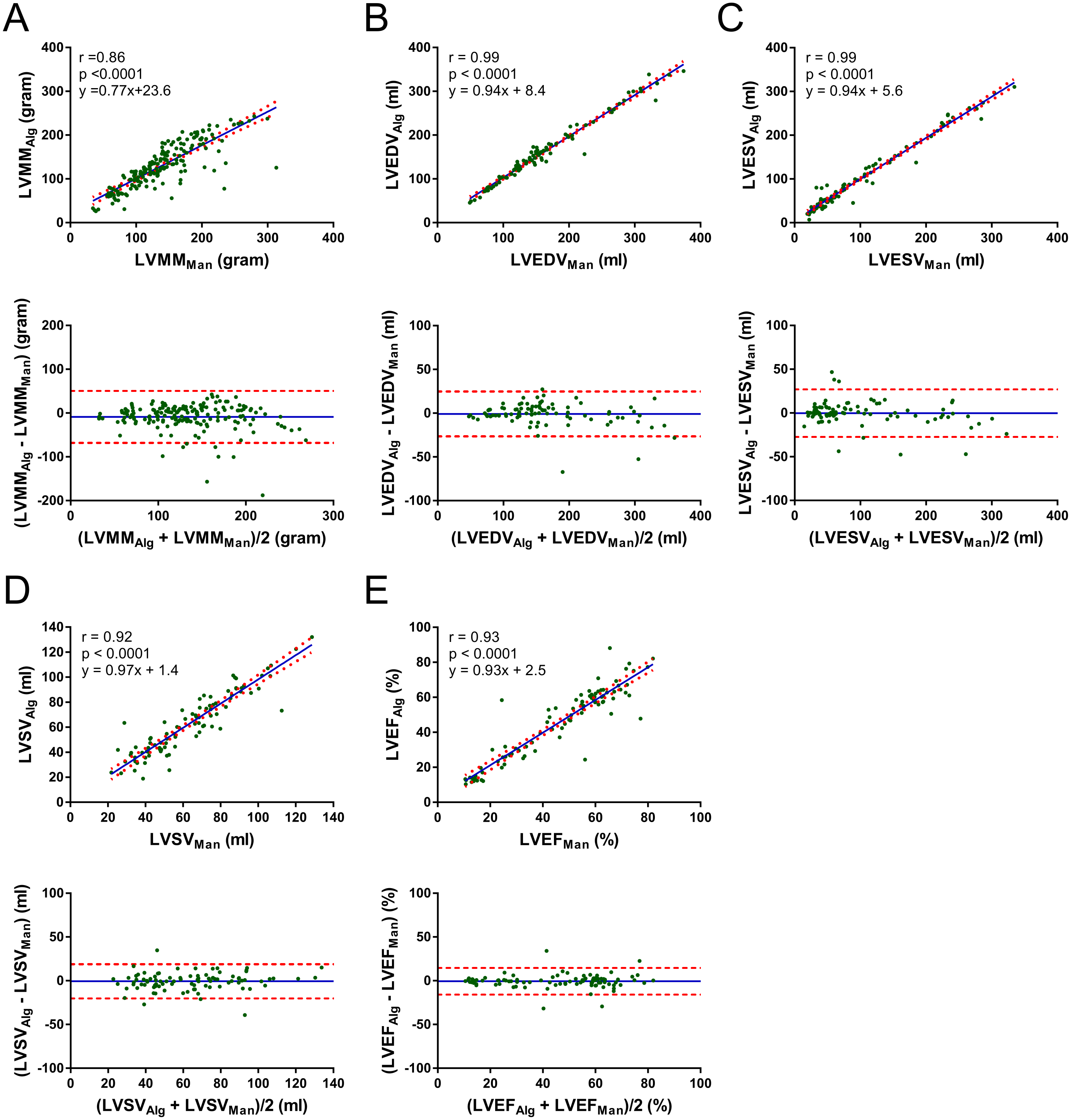
Continuous variables were expressed as mean ± standard deviation (Mean ± SD). DSC provided by the proposed approach was compared with the other comparative methods using paired t-tests. Algorithm LV function measurement errors were compared using paired t-tests. Relationships and agreement for algorithm vs. manual LV indices were assessed using Pearson correlation coefficients (r, 95% confidence intervals [CI]) and Bland-Altman analyses (with 95% limits of agreement [LOA]). Fisher’s z-transformation [35] was used to compare the correlation coefficients provided by each algorithm vs. manual analyses. Shapiro–Wilk tests were used to assess if the data can be modeled by a normal distribution and when data were not normally distributed, nonparametric tests were performed. We used GraphPad Prism v7.00 (GraphPad Software Inc., San Diego, CA, USA) for all the statistical analyses. Results were considered significant when the probability of making a two-tailed type I error was less than 5% (p < 0.05).

3. Results

Figure 2 shows segmentation of different regions of the heart at end-diastole and end-systole for three ACDC test subjects using the proposed algorithm (left) and the combined method (right).

We observed that direct application of the trained model to the 10 fine-tuning subjects yielded DSC of 0.77, 0.90 and ASSD of 2.32 mm, 2.88 mm for LVM, LVC; these accuracies were improved to 0.82, 0.92 for DSC and 1.97 mm, 1.91 mm for ASSD by the proposed CKC algorithm (data not shown), which were used to fine-tune the pre-trained model. As shown in

Table 1. LV myocardium and cavity segmentation accuracy (mean ± SD) for n = 180 images from 90 previously unseen ACDC test subjects.

	DSC ([0, 1])		ASSD (mm)
Methods	LVM	LVV	LVM	LVC
Proposed	0.81 ± 0.09	0.90 ± 0.09	2.04 ± 1.77	1.82 ± 2.18
Naive	0.74 ± 0.12 *	0.87 ± 0.12 *	2.43 ± 2.16 *	2.40 ± 2.58 *
Combined	0.78 ± 0.08 *	0.87 ± 0.12 *	2.71 ± 2.50 *	2.87 ± 2.61 *
DeepLab	0.26 ± 0.18 *	0.32 ± 0.27 *	18.60 ± 17.48 *	17.33 ± 12.37 *

DSC: Dice-similarity-coefficient, ASSD: average-symmetric-surfaced-distance; LVM: left ventricle myocardium, LVC: left ventricle cavity; *: p < 0.0001 when compared with the proposed algorithm.

, for the 90 test subjects the proposed algorithm yielded DSC of 0.81 ± 0.09 for LVM and 0.90 ± 0.09 for LVC. Meanwhile, the combined method generated DSC of 0.78 ± 0.08 and 0.87 ± 0.12 for the two regions, higher than the naive method and DeepLabV3+. Similarly, the proposed algorithm yielded substantially lower ASSD compared with the naive method, which further outperformed the combined method and DeepLabV3+. Of note, the DSC and ASSD provided by our approach were significantly different from each of the other algorithms (p < 0.0001), and the naive method demonstrated higher overall segmentation accuracy than the combined method and DeepLabV3+. As shown in

Table A1. Effects of Monte-Carlo dropout, spatial augmentation, and style-intensity augmentation on U-net training using the LVSC dataset. The three components were combined during U-net training (optimal implementation) and the trained U-net models were directly applied to the 90 ACDC test subjects (n = 180 images) for DSC and ASSD (mean ± SD) calculation.

			DSC ([0, 1])		ASSD (mm)
MCD	Spa. Aug.	Sty.-Int. Aug.	LVM	LVC	LVM	LVC
ine ✗	✗	✗	0.33 ± 0.22	0.46 ± 0.30	16.85 ± 21.52	15.28 ± 18.02
✗	✗	✓	0.49 ± 0.18	0.68 ± 0.22	8.38 ± 7.33	8.55 ± 8.69
✗	✓	✗	0.73 ± 0.12	0.85 ± 0.14	2.92 ± 2.86	3.34 ± 3.48
✗	✓	✓	0.77 ± 0.07	0.87 ± 0.11	2.39 ± 2.05	2.80 ± 2.49
✓	✗	✗	0.34 ± 0.21	0.49 ± 0.29	11.30 ± 16.93	9.97 ± 15.36
✓	✗	✓	0.55 ± 0.17	0.71 ± 0.21	7.47 ± 7.00	7.37 ± 8.22
✓	✓	✗	0.75 ± 0.11	0.87 ± 0.12	2.30 ± 1.64	2.39 ± 1.85
✓	✓	✓	0.78 ± 0.08	0.87 ± 0.12	2.71 ± 2.50	2.87 ± 2.61

✗: a component is not used., ✓: a component is used. DSC: Dice-similarity-coefficient, ASSD: average-symmetric-surfaced-distance; LVM: left ventricle myocardium; LVC: left ventricle cavity; MCD: Monte-Carlo dropout; Spa. Aug.: spatial augmentation; Sty.-Int. Aug.: style-intensity augmentation.

in Appendix A, MCD, spatial augmentation, and style-intensity augmentation each improved the segmentation accuracy and the combination of the three components, which constitutes the combined method, provided the highest segmentation accuracy among all the possible combinations.

Table 2. Algorithm and manual LV function measurements (mean ± SD) for n = 180 images from 90 previously unseen ACDC test subjects.

	Manual	Proposed	Naive	Combined	DeepLab
LVMM (g) ¥	138.1 ± 54.3	129.3 ± 49.8${}_{0.1976}$	110.8 ± 48.2${}_{<0.0001}$	154.4 ± 83.6${}_{0.0023}$	46.4 ± 34.7${}_{<0.0001}$
LVEDV (mL)	163.8 ± 75.2	162.9 ± 72.0${}_{0.8015}$	174.6 ± 74.5${}_{<0.0001}$	175.8 ± 72.8${}_{<0.0001}$	71.8 ± 69.3${}_{<0.0001}$
LVESV (mL)	99.4 ± 80.4	99.2 ± 76.7${}_{0.8631}$	108.2 ± 80.0${}_{<0.0001}$	118.4 ± 76.2${}_{<0.0001}$	58.3 ± 62.1${}_{<0.0001}$
LVSV (mL)	64.4 ± 24.6	63.7 ± 25.8${}_{0.6617}$	66.5 ± 31.5${}_{0.0734}$	57.4 ± 25.9${}_{<0.0001}$	13.5 ± 24.2${}_{<0.0001}$
LVEF (%)	46.2 ± 20.4	45.5 ± 20.5${}_{0.2495}$	43.0 ± 23.6${}_{0.0059}$	36.7 ± 18.4${}_{<0.0001}$	−4.4 ± 142.2${}_{<0.0001}$

VMM: LV myocardium mass (g); LVEDV: LV end-diastolic volume (mL); LVESV: LV end-systolic volume (mL); LVSV: LV stroke volume (mL); LVEF: LV ejection fraction (%); ^¥: n = 180 images from 90 subject; p-values for comparison of algorithm vs. manual LV indices are shown in subscripts.

summarizes the LV functional parameters generated by manual and algorithm segmentation, illustrating that LV function measurements provided by the proposed approach are closer to manual results compared with the other methods. For example, paired t-tests showed that LV indices provided by the proposed approach were not significantly different from manual measurements, whereas the measurements generated by the naive and combined method were significantly different from manual LVMM (Proposed: p = 0.1976; Naive: p < 0.0001; Combined: p = 0.0023), LVEDV (Proposed: p = 0.8015; Naive: p < 0.0001; Combined: p < 0.0001), LVESV (Proposed: p = 0.8631; Naive: p < 0.0001; Combined: p < 0.0001), LVSV (Proposed: p = 0.6617; Naive: p = 0.0734; Combined: p < 0.0001), and LVEF (Proposed: p = 0.2495; Naive: p = 0.0059; Combined: p < 0.0001).

Table 3. Relationships (Pearson r and []=95% CI) for algorithm vs. manual LV function measurements for n = 180 images from 90 previously unseen ACDC test subjects.

Pearson (r, 95% CI)	Proposed vs. Manual	Naive vs. Manual	Combined. vs. Manual	DeepLab vs. Manual
ine LVMM (g) ¥	0.86 ([0.80, 0.90])	0.79 ([0.73, 0.84])	0.41 ([0.28, 0.52])	0.47 ([0.35, 0.58])
LVEDV (mL)	0.99 ([0.98, 0.99])	0.98 ([0.97, 0.99])	0.99 ([0.99, 0.99])	0.57 ([0.41, 0.69])
LVESV (mL)	0.99 ([0.98, 0.99])	0.98 ([0.97, 0.99])	0.97 ([0.96, 0.98])	0.65 ([0.51, 0.75])
LVSV (mL)	0.92 ([0.88, 0.95])	0.84 ([0.76, 0.89])	0.83 ([0.75, 0.89])	0.13 ([−0.08, 0.33])
LVEF (%)	0.93 ([0.89, 0.95])	0.75 ([0.65, 0.83])	0.76 ([0.65, 0.83])	0.08 ([−0.13, 0.28])

VMM: LV myocardium mass (g); LVEDV: LV end-diastolic volume (mL); LVESV: LV end-systolic volume (mL); LVSV: LV stroke volume (mL); LVEF: LV ejection fraction (%); ^¥: n = 180 images from 90 subject.

and Figure 3 show that there were strong and significant correlations between the proposed algorithm and the naive method vs. manual analyses of LVMM (Proposed: r = 0.86, p < 0.0001; Naive: r = 0.79, p < 0.0001), LVEDV (Proposed: r = 0.99, p < 0.0001; Naive: r = 0.98, p < 0.0001), LVESV (Proposed: r = 0.99, p < 0.0001; Naive: r = 0.98, p < 0.0001), LVSV (Proposed: r = 0.92, p < 0.0001; Naive: r =0.84, p < 0.0001), and LVEF (Proposed: r = 0.93, p < 0.0001; Naive: r = 0.75, p < 0.0001). Please note that the correlations between the naive and combined methods vs. manual measurements were very similar for all the LV indices except for LVMM. Fisher’s z-transformations showed that the correlations for the proposed algorithm and the naive method vs. manual measurements were significantly different for LVMM (p = 0.0366), LVEDV (p = 0.0214), LVESV (p = 0.0214), LVSV (p = 0.0151), and LVEF (p < 0.0001). Similar results were observed when comparing the correlations yielded by the proposed algorithm and the combined method.

Figure 3 also shows the quantitative agreement between the proposed algorithm and manual LV indices. Bland-Altman analyses indicated that there was promising agreement between the proposed algorithm and manual LVMM (bias = −8.8 ± 30.3 g, 95% LOA = [−68.1, 50.5] g), LVEDV (bias = −0.9 ± 13.1 mL, 95% LOA = [−26.6, 24.8] mL), LVESV (bias = −0.2 ± 13.8 mL, 95% LOA = [−27.3, 26.9] mL), LVSV (bias = −0.7 ± 10.0 mL, 95% LOA = [−20.2, 18.9] mL), and LVEF (bias = −0.6 ± 7.8%, 95% LOA = [−15.9%, 14.6%]). In contrast, the naive and combined methods yielded greater biases and wider 95% LOAs for LVMM (Naive: bias = −27.3 ± 33.3 g, 95% LOA = [−92.5, 37.9] g; Combined: bias =16.4 ± 79.0 g, 95% LOA = [−138.5, 171.3] g); LVEDV (Naive: bias=10.9 ± 14.5 mL, 95% LOA = [−17.5, 39.2] mL; Combined: bias = 12.0 ± 11.2 mL, 95% LOA = [−10.0, 34.0] mL), LVESV (Naive: bias = 8.8 ± 16.7 mL, 95% LOA = [−24.0, 41.5] mL; Combined: bias = 19.0 ± 18.1 mL, 95% LOA = [−16.4, 54.4] mL), LVSV (Naive: bias = 2.1 ± 17.4 mL, 95% LOA = [−31.9, 36.1] mL; Combined: bias = −7.0 ± 14.7 mL, 95% LOA = [−35.8, 21.8] mL), and LVEF (Naive: bias = −3.1 ± 15.8%, 95% LOA = [−34.0%, 27.7%]; Combined: bias = −9.5 ± 13.6%, 95% LOA = [−36.1%, 17.2%]).

For the proposed algorithm and the naive method, U-net training/pre-training was completed in approximately 5 h. The fine-tuning procedure required an additional ∼12 min, including 10 s to post-process each image using the CKC algorithm and 10 min to update the U-net parameters. The combined method required ∼15 h for training and DeepLabV3+ required ∼5 h. For all the trained/fine-tuned models, inference of a new 2D cine image stack required ∼1 s.

4. Discussion

Deep learning is emerging to potentially transform cardiac imaging workflow and clinical patient care. Here, we developed an approach to employing a trained CNN for LV segmentation and function evaluation in an independent cardiac cine MRI dataset. For a dataset of 180 cine MR images from 90 subjects with various cardiac disease, we made the following observations: (1) improved segmentation accuracy in the independent dataset; (2) strong correlations between the proposed approach and manual analyses of LV indices; and (3) rapid and fully automated fine-tuning procedure without needing manual labels for the independent dataset.

Cine MRI has been routinely performed for evaluation of LV structure and function in cardiovascular MR exams. Deep learning and machine leaning have demonstrated promise in several aspects of the cardiac research and clinical workflow, including but not limited to prediction of cardiac left ventricular kinematics and boundaries [36], classification of cardiac arrhythmias from electrocardiogram [37], and detection of cardiac structure and structural abnormalities [38]. However, direct application of a trained model to a previously unseen dataset often yields suboptimal performance [3,8,39]. For example, direct application of a CNN trained on a large cine MRI dataset of 4275 subjects [8] to 20 patients in a previously unseen ACDC dataset yielded DSC of 0.65 for LVM and 0.74 for LVC. Previous studies showed that DSC is usually sensitive to small differences when the segmented object is relatively small and not very sensitive to errors when the object is relatively large [40]. We note that the size of LVM is generally smaller than the LVC at end-diastole although the differences between the two regions are smaller at end-systole. A recent study [9] investigated the variabilities of intra and inter-observer manual segmentation. The authors reported greater DSC of 0.956–0.967 for LVC and 0.870–0.900 for LVM at end-diastole, and similarly, these were 0.898–0.941 and 0.891–0.917 at end-systole. The robustness of manual segmentation and the substantially lower algorithm DSC [8] than repeated manual analyses (0.65 vs. 0.870–917) suggest that manual segmentation errors have a minimal effect in this case. In addition, the training and testing datasets used by Bai et al. [8] differ substantially as the training dataset mainly consists of healthy volunteers whereas the testing dataset comprise patients with diverse cardiac pathologies, which affect the appearance of the myocardium in MR images. Based on the literature and our experience, we think that the relatively low DSC for LVM than LVC (0.65 vs. 0.74) reported by Bai et al. [8] is mainly caused by the combined effects of the large differences between training and testing datasets, the relatively small size, hollow shape, and image signal intensity inhomogeneity in the LVM compared with LVC. However, this warrants further investigation. Nonetheless, the initial suboptimal accuracies [8] were later improved by employing 80 manually segmented subjects in the ACDC dataset for fine-tuning. Previous studies [4,41] and our efforts have shown that manual segmentation of a 3D cardiac MR volume with 10–15 slices typically requires 20–30 min. This lengthy procedure requires experience and expertise from examiners, introduces user variability, and is not compatible with efficient research and clinical workflow. Similarly, another study [3] applied a pre-trained state-of-the-art CNN (1st place winner in the ACDC segmentation challenge) to 40 ACDC subjects and achieved DSC of 0.78 for LVM and 0.86 LVC. Compared with these previous works, our approach yielded greater DSC of 0.81 for LVM and 0.90 for LVC without requiring manual segmentation of the fine-tuning datasets. In our future work, we will compare the results from this study with that by fine-tuning the proposed algorithm framework using manually segmented unseen dataset in terms of segmentation accuracy and time. In addition, the derived LV function measurements provided by our approach were strongly correlated with expert manual analyses with no significant differences between the techniques (p = 0.1976–0.8631, Table 2). This is important because our approach implemented fully automated transfer learning to segment an independent cardiac cine MR dataset acquired using a different MR system at a different location in patients with different cardiac diseases without requiring manual segmentation of the target dataset, potentially enabling efficient clinical workflow and facilitating broader use of deep learning for a wide range of applications.

We also implemented a combined method that employed state-of-the-art style-intensity augmentation techniques [17] to address the domain shift issue, which had performed well for breast segmentation in different MRI datasets. Compared with our approach, the optimized implementation of the combined method yielded lower DSC of 0.78 for LVM and 0.87 for LVC with substantially greater ASSD, as shown in Table 1. In another study [18], the authors tackled a similar problem by developing a series of stacked transformations that performed extensive data augmentation (sharpening, blurring, adding noise, changing brightness/contrast, intensity perturbation, rotation, scaling, deformation) during network training. For eight public MRI/ultrasound datasets, the authors achieved improved segmentation accuracy with the use of the proposed data augmentation techniques. These studies [17,18] showed that advanced and extensive data augmentation techniques yielded higher segmentation performance than adversarial learning-based domain-adaptation techniques. Surprisingly, the naive method generally outperformed the combined method for segmentation accuracy measurements (except for DSC for LVM) but the correlations of LV function measurements with manual results were comparable. This warrants further investigation. Of note, the well-known DeepLabV3+ algorithm [30] performed poorly in this work (see Figure A1), further highlighting the challenges of domain shift for medical image segmentation. In fact, we previously trained the DeepLabV3+ model on 50 subjects from the UK Biobank dataset and applied the model to segment 50 previously unseen ACDC subjects. We achieved DSC of 0.437 for LVM and 0.568 for LVC. Similarly, we trained the DeepLabV3+ model on 50 ACDC subjects and tested the model on 50 subjects from the UK Biobank dataset. We obtained DSC of 0.745 for LVM AND 0.813 for LVC. Please note that these results are excluded in the final version of our previous paper [3] as suggested by the reviewers. In a recent study of lung MRI segmentation [23], we achieved DSC of 0.872 and 0.701 by training the DeepLabV3+ model on one dataset and testing the model on another different dataset. Collectively, these and other studies suggest the inability of deep learning, including DeepLabV3+ and other state-of-the-art models, to deal with the domain shift issue for medical image segmentation. Our approach outperformed the naive method and a combined method that used state-of-the-art data augmentation techniques [17] and differs from the other methods [18,31] in that in addition to comprehensive data augmentation, we implemented Monte-Carlo dropout to mitigate overfitting and a CKC algorithm to automatically update the “annotations" of the fine-tuning subjects. Previous studies [3,24] demonstrated the effectiveness of using CKC to improve CNN initial segmentation and here we substantially extended the previous work by demonstrating its utility in a new application, whereby the CKC post-processing results were incorporated to effectively tune the trained model to segment an independent cardiac cine MRI dataset. The proposed framework is relatively independent from commonly used domain adaptation and data augmentation techniques. Therefore, we think that our approach could be combined with these methods to address the domain shift issue, which represents an advantage of our approach that will be further investigated in future work.

Although our approach was based on a U-net implemented with Monte-Carlo dropout and a recently developed CKC algorithm, this work differs from other cardiac image segmentation methods developed to tackle a similar issue with higher performance for LV segmentation and biomarker quantification. In addition, the promise of our approach was demonstrated in the context of a U-net, which has been widely used for numerous applications, suggesting the generalizability of our framework for a broad range of segmentation tasks that involve a U-net. The improved segmentation generalizability may stem from the combination of the advantages of deep-learning and machine-learning methods without a deep architecture. As a result, both deep and shallow image features can be learned or employed, and the power of data-driven and rule-based segmentation methods was aggregated, potentially mitigating the limitations of the individual methods. However, further investigation of this is warranted. Efforts that can further improve the performance of our proposed approach including: (1) applying the CKC algorithm only to the fine-tuning subjects with problematic segmentation; (2) automatically selecting the datasets with acceptable CKC segmentation for CNNfine-tuning; and (3) adding a few more new unlabeled datasets for each iteration. We think that these strategies may be optimized and implemented in parallel to for potentially greater robustness. Regardless, the results realized here suggest that our approach provides a way to improve deep-learning segmentation generalizability without increasing the difficulties of algorithm interpretability, a major concern facing the community [42], and may facilitate broader use and translation of deep-learning techniques for research and clinical care.

We acknowledge several study limitations. First, the segmentation accuracy of our approach is lower than CNNs trained and tested on the same datasets. However, here we focus on adapting a trained CNN for segmentation of previously unseen cardiac MRI datasets, which is particularly challenging and requires urgent solution. Importantly, we achieved segmentation accuracies higher than two state-of-the-art segmentation methods (a combined method that employed style-intensity augmentation and DeepLabV3+) and LV function measurements that were strongly correlated with manual results. We note that the basal and apical slices of the heart are difficult to segment due to poor image qualities and the complexity of cardiac structures, which represent some of the major challenges facing the community. In addition, the proposed algorithm was validated on a retrospective dataset and the effectiveness of this approach warrants a prospective evaluation with datasets from different centers, MR scanners, imaging protocols, and disease phenotypes.

5. Conclusions

In conclusion, we developed a way to employ a pre-trained neural network to segment previously unseen cardiac MR datasets without requiring manual annotations of the unseen datasets for fine-tuning. For a clinical dataset of patients with diverse cardiac disease, we achieved LV segmentation and function evaluation accuracy and precision that may be suitable for research and clinical use. As such, our approach may facilitate the translation and use of deep learning in cardiac imaging workflow.

References

1. Flachskampf, F.A.; Biering-Sørensen, T.; Solomon, S.D.; Duvernoy, O.; Bjerner, T.; Smiseth, O.A. Cardiac imaging to evaluate left ventricular diastolic function. JACC Cardiovasc. Imaging 2015, 8, 1071–1093. [Google Scholar] [CrossRef] [PubMed] [Green Version]
2. Members, W.C.; Hundley, W.G.; Bluemke, D.A.; Finn, J.P.; Flamm, S.D.; Fogel, M.A.; Friedrich, M.G.; Ho, V.B.; Jerosch-Herold, M.; Kramer, C.M.; et al. ACCF/ACR/AHA/NASCI/SCMR 2010 expert consensus document on cardiovascular magnetic resonance: A report of the American College of Cardiology Foundation Task Force on Expert Consensus Documents. Circulation 2010, 121, 2462–2508. [Google Scholar] [CrossRef] [PubMed]
3. Guo, F.; Ng, M.; Goubran, M.; Petersen, S.E.; Piechnik, S.K.; Neubauer, S.; Wright, G. Improving cardiac MRI convolutional neural network segmentation on small training datasets and dataset shift: A continuous kernel cut approach. Med. Image Anal. 2020, 61, 101636. [Google Scholar] [CrossRef] [PubMed]
4. Petitjean, C.; Dacher, J.N. A review of segmentation methods in short axis cardiac MR images. Med. Image Anal. 2011, 15, 169–184. [Google Scholar] [CrossRef] [Green Version]
5. Peng, P.; Lekadir, K.; Gooya, A.; Shao, L.; Petersen, S.E.; Frangi, A.F. A review of heart chamber segmentation for structural and functional analysis using cardiac magnetic resonance imaging. Magn. Reson. Mater. Phys. Biol. Med. 2016, 29, 155–195. [Google Scholar] [CrossRef] [PubMed] [Green Version]
6. Shen, D.; Wu, G.; Suk, H.I. Deep learning in medical image analysis. Annu. Rev. Biomed. Eng. 2017, 19, 221–248. [Google Scholar] [CrossRef] [Green Version]
7. Leiner, T.; Rueckert, D.; Suinesiaputra, A.; Baeßler, B.; Nezafat, R.; Išgum, I.; Young, A.A. Machine learning in cardiovascular magnetic resonance: Basic concepts and applications. J. Cardiovasc. Magn. Reson. 2019, 21, 1–14. [Google Scholar] [CrossRef] [Green Version]
8. Bai, W.; Sinclair, M.; Tarroni, G.; Oktay, O.; Rajchl, M.; Vaillant, G.; Lee, A.M.; Aung, N.; Lukaschuk, E.; Sanghvi, M.M.; et al. Automated cardiovascular magnetic resonance image analysis with fully convolutional networks. J. Cardiovasc. Magn. Reson. 2018, 20, 65. [Google Scholar] [CrossRef] [Green Version]
9. Bernard, O.; Lalande, A.; Zotti, C.; Cervenansky, F.; Yang, X.; Heng, P.A.; Cetin, I.; Lekadir, K.; Camara, O.; Ballester, M.A.G.; et al. Deep learning techniques for automatic MRI cardiac multi-structures segmentation and diagnosis: Is the problem solved? IEEE Trans. Med. Imaging 2018, 37, 2514–2525. [Google Scholar] [CrossRef]
10. Chen, C.; Qin, C.; Qiu, H.; Tarroni, G.; Duan, J.; Bai, W.; Rueckert, D. Deep Learning for Cardiac Image Segmentation: A Review. Front. Cardiovasc. Med. 2020, 7, 25. [Google Scholar] [CrossRef]
11. Yan, W.; Wang, Y.; Gu, S.; Huang, L.; Yan, F.; Xia, L.; Tao, Q. The Domain Shift Problem of Medical Image Segmentation and Vendor-Adaptation by Unet-GAN. In International Conference on Medical Image Computing and Computer-Assisted Intervention; Springer: Cham, Switzerland, 2019; pp. 623–631. [Google Scholar]
12. Tzeng, E.; Hoffman, J.; Saenko, K.; Darrell, T. Adversarial discriminative domain adaptation. In Proceedings of the IEEE Conference on Computer Vision and Pattern Recognition, Honolulu, HI, USA, 21–26 July 2017; pp. 7167–7176. [Google Scholar]
13. Zhu, Y.; Fahmy, A.S.; Duan, C.; Nakamori, S.; Nezafat, R. Automated Myocardial T2 and Extracellular Volume Quantification in Cardiac MRI Using Transfer Learning—Based Myocardium Segmentation. Radiol. Artif. Intell. 2020, 2, e190034. [Google Scholar] [CrossRef] [PubMed]
14. Huo, Y.; Xu, Z.; Moon, H.; Bao, S.; Assad, A.; Moyo, T.K.; Savona, M.R.; Abramson, R.G.; Landman, B.A. Synseg-net: Synthetic segmentation without target modality ground truth. IEEE Trans. Med. Imaging 2018, 38, 1016–1025. [Google Scholar] [CrossRef] [PubMed]
15. Chen, C.; Dou, Q.; Chen, H.; Qin, J.; Heng, P.A. Unsupervised bidirectional cross-modality adaptation via deeply synergistic image and feature alignment for medical image segmentation. IEEE Trans. Med. Imaging 2020, 39, 2494–2505. [Google Scholar] [CrossRef] [PubMed] [Green Version]
16. Krizhevsky, A.; Sutskever, I.; Hinton, G.E. Imagenet classification with deep convolutional neural networks. Commun. ACM 2017, 60, 84–90. [Google Scholar] [CrossRef]
17. Hesse, L.S.; Kuling, G.; Veta, M.; Martel, A. Intensity augmentation to improve generalizability of breast segmentation across different MRI scan protocols. IEEE Trans. Biomed. Eng. 2020, 68, 759–770. [Google Scholar] [CrossRef]
18. Zhang, L.; Wang, X.; Yang, D.; Sanford, T.; Harmon, S.; Turkbey, B.; Wood, B.J.; Roth, H.; Myronenko, A.; Xu, D.; et al. Generalizing deep learning for medical image segmentation to unseen domains via deep stacked transformation. IEEE Trans. Med. Imaging 2020, 39, 2531–2540. [Google Scholar] [CrossRef]
19. Guo, F.; Ng, M.; Roifman, I.; Wright, G. Cardiac MRI Left Ventricular Segmentation and Function Quantification Using Pre-trained Neural Networks. In International Conference on Functional Imaging and Modeling of the Heart; Springer: Cham, Switzerland, 2021; pp. 46–54. [Google Scholar]
20. Radau, P.; Lu, Y.; Connelly, K.; Paul, G.; Dick, A.; Wright, G. Evaluation framework for algorithms segmenting short axis cardiac MRI. MIDAS J.-Card. MR Left Ventricle Segmentation Chall. 2009, 49. [Google Scholar] [CrossRef]
21. Ronneberger, O.; Fischer, P.; Brox, T. U-net: Convolutional networks for biomedical image segmentation. In International Conference on Medical Image Computing and Computer-Assisted Intervention; Springer: Cham, Switzerland, 2015; pp. 234–241. [Google Scholar]
22. Gal, Y.; Ghahramani, Z. Dropout as a bayesian approximation: Representing model uncertainty in deep learning. In Proceedings of the 33rd International Conference on Machine Learning, New York, NY, USA, 20–22 June 2016; pp. 1050–1059. [Google Scholar]
23. Guo, F.; Capaldi, D.P.; McCormack, D.G.; Fenster, A.; Parraga, G. Ultra-short Echo-time Magnetic Resonance Imaging Lung Segmentation with Under-Annotations and Domain Shift. Med. Image Anal. 2021, 72, 102107. [Google Scholar] [CrossRef]
24. Guo, F.; Ng, M.; Wright, G. Cardiac cine MRI left ventricle segmentation combining deep learning and graphical models. In Medical Imaging 2020: Image Processing; International Society for Optics and Photonics: Bellingham, WA, USA, 2020; Volume 11313. [Google Scholar]
25. Guo, F.; Krahn, P.R.; Escartin, T.; Roifman, I.; Wright, G. Cine and late gadolinium enhancement MRI registration and automated myocardial infarct heterogeneity quantification. Magn. Reson. Med. 2021, 85, 2842–2855. [Google Scholar] [CrossRef]
26. Tang, M.; Ben Ayed, I.; Marin, D.; Boykov, Y. Secrets of grabcut and kernel k-means. In Proceedings of the IEEE International Conference on Computer Vision, Santiago, Chile, 7–13 December 2015; pp. 1555–1563. [Google Scholar]
27. Yuan, J.; Bae, E.; Tai, X.C. A study on continuous max-flow and min-cut approaches. In Proceedings of the 2010 IEEE Computer Society Conference on Computer Vision and Pattern Recognition, San Francisco, CA, USA, 13–18 June 2010; pp. 2217–2224. [Google Scholar]
28. Guo, F.; Yuan, J.; Rajchl, M.; Svenningsen, S.; Capaldi, D.P.; Sheikh, K.; Fenster, A.; Parraga, G. Globally optimal co-segmentation of three-dimensional pulmonary 1H and hyperpolarized 3He MRI with spatial consistence prior. Med. Image Anal. 2015, 23, 43–55. [Google Scholar] [CrossRef]
29. Jackson, P.T.; Abarghouei, A.A.; Bonner, S.; Breckon, T.P.; Obara, B. Style augmentation: Data augmentation via style randomization. In Proceedings of the CVPR Workshops, Long Beach, CA, USA, 16–21 June 2019; pp. 83–92. [Google Scholar]
30. Chen, L.C.; Zhu, Y.; Papandreou, G.; Schroff, F.; Adam, H. Encoder-decoder with atrous separable convolution for semantic image segmentation. In Proceedings of the European conference on computer vision (ECCV), Munich, Germany, 8–14 September 2018; pp. 801–818. [Google Scholar]
31. Guo, F.; Ng, M.; Wright, G. Cardiac MRI left ventricle segmentation and quantification: A framework combining U-Net and continuous max-flow. In International Workshop on Statistical Atlases and Computational Models of the Heart; Springer: Cham, Switzerland, 2018; pp. 450–458. [Google Scholar]
32. Nai, Y.H.; Teo, B.W.; Tan, N.L.; O’Doherty, S.; Stephenson, M.C.; Thian, Y.L.; Chiong, E.; Reilhac, A. Comparison of metrics for the evaluation of medical segmentations using prostate MRI dataset. Comput. Biol. Med. 2021, 134, 104497. [Google Scholar] [CrossRef]
33. Maier-Hein, L.; Eisenmann, M.; Reinke, A.; Onogur, S.; Stankovic, M.; Scholz, P.; Arbel, T.; Bogunovic, H.; Bradley, A.P.; Carass, A.; et al. Why rankings of biomedical image analysis competitions should be interpreted with care. Nat. Commun. 2018, 9, 1–13. [Google Scholar] [CrossRef] [PubMed] [Green Version]
34. Grothues, F.; Smith, G.C.; Moon, J.C.; Bellenger, N.G.; Collins, P.; Klein, H.U.; Pennell, D.J. Comparison of interstudy reproducibility of cardiovascular magnetic resonance with two-dimensional echocardiography in normal subjects and in patients with heart failure or left ventricular hypertrophy. Am. J. Cardiol. 2002, 90, 29–34. [Google Scholar] [CrossRef]
35. Kirby, M.; Svenningsen, S.; Owrangi, A.; Wheatley, A.; Farag, A.; Ouriadov, A.; Santyr, G.E.; Etemad-Rezai, R.; Coxson, H.O.; McCormack, D.G.; et al. Hyperpolarized 3He and 129Xe MR imaging in healthy volunteers and patients with chronic obstructive pulmonary disease. Radiology 2012, 265, 600–610. [Google Scholar] [CrossRef]
36. Damen, F.W.; Newton, D.T.; Lin, G.; Goergen, C.J. Machine Learning Driven Contouring of High-Frequency Four-Dimensional Cardiac Ultrasound Data. Appl. Sci. 2021, 11, 1690. [Google Scholar] [CrossRef]
37. Lee, H.; Yoon, T.; Yeo, C.; Oh, H.; Ji, Y.; Sim, S.; Kang, D. Cardiac Arrhythmia Classification Based on One-Dimensional Morphological Features. Appl. Sci. 2021, 11, 9460. [Google Scholar] [CrossRef]
38. Komatsu, M.; Sakai, A.; Komatsu, R.; Matsuoka, R.; Yasutomi, S.; Shozu, K.; Dozen, A.; Machino, H.; Hidaka, H.; Arakaki, T.; et al. Detection of cardiac structural abnormalities in fetal ultrasound videos using deep learning. Appl. Sci. 2021, 11, 371. [Google Scholar] [CrossRef]
39. Tao, Q.; Yan, W.; Wang, Y.; Paiman, E.H.; Shamonin, D.P.; Garg, P.; Plein, S.; Huang, L.; Xia, L.; Sramko, M.; et al. Deep learning–based method for fully automatic quantification of left ventricle function from cine MR images: A multivendor, multicenter study. Radiology 2019, 290, 81–88. [Google Scholar] [CrossRef] [Green Version]
40. Wong, K.C.; Moradi, M.; Tang, H.; Syeda-Mahmood, T. 3D segmentation with exponential logarithmic loss for highly unbalanced object sizes. In International Conference on Medical Image Computing and Computer-Assisted Intervention; Springer: Cham, Switzerland, 2018; pp. 612–619. [Google Scholar]
41. Wang, Y.; Zhang, Y.; Xuan, W.; Kao, E.; Cao, P.; Tian, B.; Ordovas, K.; Saloner, D.; Liu, J. Fully automatic segmentation of 4D MRI for cardiac functional measurements. Med. Phys. 2019, 46, 180–189. [Google Scholar] [CrossRef] [Green Version]
42. Rudin, C. Stop explaining black box machine learning models for high stakes decisions and use interpretable models instead. Nat. Mach. Intell. 2019, 1, 206–215. [Google Scholar] [CrossRef] [Green Version]
Figure 1. Schematic of the proposed algorithm pipeline for cardiac MR image segmentation using pre-trained CNNs. A trained CNN was applied to 10 previously unseen subjects; the initial segmentation was post-processed and post-processed using a kernel-cut algorithm. The resulting segmentation was used to update the trained CNN. This procedure was iterated till convergence to derive the final CNN model, which was applied to the unseen test dataset for LV function evaluation. Please note that no manual annotation of the unseen dataset was required in this procedure.
Applsci 12 02627 g001
Figure 2. Representative segmentation of different regions of the heart at end-systole and end-diastole for three unseen ACDC test subjects (Subject1, Subject2, and Subject3) using the proposed (left) and the combined (right) methods. Algorithm and manual segmentation are shown in purple and yellow, respectively. ED: end-diastole; ES: end-systole.
Applsci 12 02627 g002
Figure 3. Relationships and agreement between the proposed algorithm vs. manual measurements of LVMM (A), LVEDV (B), LVESV (C), LVSV (D), and LVEF (E) (n = 180 images from 90 subjects). Linear regression and Bland-Altman analyses of algorithm vs. manual LV indices are shown in the top and bottom plots, respectively. A l g : algorithm results; M a n : manual results. Solid lines (blue) indicate the biases and dotted lines (red) represent the 95% limits of agreement.
Applsci 12 02627 g003