Longitudinal Mode System Identification of an Insect-like Tailless Flapping-Wing Micro Air Vehicle Using Onboard Sensors

Featured Application

This paper presents the development of a longitudinal mode dynamic model via experiments of insect-like tailless flapping-wing micro air vehicles (FWMAVs).

Abstract

In this paper, model parameter identification results are presented for a longitudinal mode dynamic model of an insect-like tailless flapping-wing micro air vehicle (FWMAV) using angle and angular rate data from onboard sensors only. A gray box model approach with indirect method was utilized with adaptive Gauss–Newton, Levenberg–Marquardt, and gradient search identification methods. Regular and low-frequency reference commands were mainly used for identification since they gave higher fit percentages than irregular and high-frequency reference commands. Dynamic parameters obtained using three identification methods with two different datasets were similar to each other, indicating that the obtained dynamic model was sufficiently reliable. Most of the identified dynamic model parameters had similar values to the computationally obtained ones, except stability derivatives for pitching moment with forward velocity and pitching rate variations. Differences were mainly due to certain neglected body, nonlinear dynamics, and the shift of the center of gravity. Fit percentage of the identified dynamic model (~49%) was more than two-fold higher than that of the computationally obtained one (~22%). Frequency domain analysis showed that the identified model was much different from that of the computationally obtained one in the frequency range of 0.3 rad/s to 5 rad/s, which affected transient responses. Both dynamic models showed that the phase margin was very low, and that it should be increased by a feedback controller to have a robustly stable system. The stable dominant pole of the identified model had a higher magnitude which resulted in faster responses. The identified dynamic model exhibited much closer responses to experimental flight data in pitching motion than the computationally obtained dynamic model, demonstrating that the identified dynamic model could be used for the design of more effective pitch angle-stabilizing controllers.

1. Introduction

Nature provides investigators with abundant insights and inspirations that aid in solving engineering problems and creating new inventions [1,2]. With the advancement of science, engineering, and technology, a growing number of robots have been designed in different shapes and sizes to mimic biological systems [3,4]. These biomimetic robots mimic animals, such as four-legged animals (quadrupeds) [5], monkeys [6], snakes [7], fish [8,9], bats [10,11], and various birds and insects [12,13,14]. These robots have diverse potential applications, ranging from simple toys to exploration robots in dangerous and hazardous environments. They have the potential to perform tasks that conventional robots cannot accomplish, such as climbing steep surfaces [15,16], maneuvering through rubble [17], and walking on uneven terrains [5]. These unique capabilities that only animals can perform have motivated many researchers to develop biomimetic robots.

The flapping-wing micro air vehicle (FWMAV) is one such type of robot. It has been popular for more than a decade [12,18,19,20]. With birds and insects as the main source of inspiration for designing robots, FWMAVs are typically categorized into bird- or insect-inspired FWMAVs. Alternatively, they are differentiated into tailed or tailless FWMAVs based on the existence of the control surface on their tails, by which the differentiation agrees with the physical configurations of birds or insects, respectively [21,22,23,24,25]. In general, birds and insects have unique flight characteristics, which can be observed from the manner in which their wings are manipulated and modulated. Compared to birds, insects normally flap with higher flapping frequency and larger stroke amplitude to produce sufficient force to fly. The flapping stroke plane of insects is nearly horizontal, which causes similar lift force to be produced during a downstroke and an upstroke, whereas the flapping stroke plane of birds is practically vertical, which causes most of the lift force to be produced during downstroke [23,24]. These flight characteristics are mimicked by FWMAVs using various approaches and engineering designs, especially for producing wing flapping motion and other kinematics to generate force and moment [19,20,26].

Unlike tailed FWMAVs, tailless FWMAVs can exhibit steady hover and high maneuverability during a flight [27], indicating their potential applications in restricted spaces. To date, several tailless FWMAV designs have successfully performed stable flight, including the Nano Hummingbird [27], RoboBee [28], Delfly Nimble [29], KUBeetle [30,31,32,33,34,35], robotic hummingbird [36], Colibri [37], NUS-Robobird [38], and Purdue Hummingbird [39]. There are some similarities between each design. Nano Hummingbird, KUBeetle, robotic hummingbird, and Colibri use only one DC motor to generate thrust through one pair of wings and a few servos to manipulate the wing kinematics for control moment generation. They are mainly different in system integration and various transmission mechanisms, such as combination of string and crankshaft [27], combination of 4-bar linkage and pulley-string [30], and combination of slider-crank and 4-bar linkage [37]. In comparison, Delfly Nimble and NUS-Robobird use two DC motors to manipulate the flapping of two pairs of wings to generate thrust and roll moments. Servos are used to adjust the relative angle of two flapping mechanisms for pitch and yaw moment generation. A different control strategy was found in Purdue Hummingbird where each wing, one left and one right, is controlled by a DC motor to realize fully decoupled and independent wing kinematics manipulation. In this way, no servos are needed because control moments are generated by changing the wing flapping range and speed. While most tailless FWMAVs with successful flights use DC motors and servos, RoboBee uses piezoelectric actuators driven with high voltage. Stabilizing tailless FWMAVs is a significantly important objective in the development of tailless FWMAVs for flying. Owing to the inherent instability of tailless FWMAVs, feedback controllers are required to stabilize them during flight. In comparison, tailed FWMAVs, such as the Microbat [40], Delfly II [41], TL-Flowerfly [42], Konkuk University Biomimetic Ornithopter [43], H2Bird Ornithopter [44], and Robird [45], have an inherent stability [46] so that they can maintain equilibrium without any active manipulation of wing or tail kinematics. Recent findings on Hawkmoth [47] have indicated that the vibration of flapping wings potentially contributes to the improved stability of large insects and FWMAVs through a passive vibrational stabilization mechanism.

Owing to their feasibility and simplicity, proportional–integral–derivative (PID) feedback controllers and their simple variants are often implemented, particularly during the early development of tailless FWMAVs [19,30,37,38]. More complex variants of PID feedback controllers incorporating different strategies (such as neural network [48], particle swarm optimization [49], and dominant pole placement [50]) and autotuning algorithms (such as optimal approach [51,52] and fuzzy adaptive [53]) are being developed for various applications. As with many biomimetic robots, tailless FWMAVs have less complicated body structures and control mechanisms than their biological counterparts. Thus, they can be considered as simplified versions of insects. However, owing to the nonlinear, time-varying, and periodic nature of these systems, describing the mechanics of tailless FWMAVs is still a considerable challenge. In addition, as tailless FWMAVs have different wing configurations [54,55,56,57], actuators, and control mechanisms [19,27,28,29,30,31,32,33,34,35,36,37,38,39], they cannot be fully generalized. Many efforts have been made to model the flapping kinematics, aerodynamics, and flight dynamics of flyers and FWMAVs. They are derived computationally or experimentally with various assumptions, ranging from time-invariant linear to nonlinear time-periodic models [58,59,60]. One of the main purposes of obtaining a dynamic model is to design a flight controller with various control techniques and schemes, such as PID [34,61], linear–quadratic–Gaussian [62], state feedback [63,64], nonlinear [65,66,67], sliding mode [68,69], robust [70,71], adaptive [72], adaptive neural network [73,74], and model-free [75]. While many dynamic models and controllers have been successfully developed, only a limited number have been implemented on tailless FWMAVs because some tailless FWMAVs cannot generate sufficient lift to perform free flight for implementation and verification.

In this study, the system identification of a tailless FWMAV called KUBeetle was conducted to improve the previously derived longitudinal mode extended dynamic model [34] and obtain a more accurate dynamic model to design a controller. The fabrication of tailless FWMAVs with successful flight makes it possible for system identification based on measured input and output data to be conducted [65,76,77,78,79,80,81,82]. This approach can potentially identify real dynamics and address the design changes of tailless FWMAVs to obtain a dynamic model with a high degree of similarity to actual systems. In a previous study [65], three single-axis closed-loop system identifications of the robotic hummingbird were conducted using a gimbal system and a Vicon motion tracking system with step reference command as the input. A second-order system was used to describe the pitch, roll, and yaw dynamic. A theoretical linear model for the piezo actuator positioning of Robobee wings’ [76] was developed using an off-board displacement laser sensor. The identified model had an error of around 5%, but it was restricted to the wing driving system. A longitudinal gray box model system identification using open-loop system identification procedures was conducted on Delfly Nimble [77]. Data were obtained using the OptiTrack motion tracking system and the onboard system with doublet input as a reference command. The obtained linear time-averaged longitudinal dynamic models for hover and forward flight up to 1 m/s showed more than 80% fit.

The majority of system identification research uses high-speed camera systems with high data rates to obtain experimental flight data. High-speed camera systems are very expensive. In addition, the camera marker balls are relatively heavy compared to the small mass of the KUBeetle (only 17.7 g), which could affect the dynamics. Moreover, there exists little difference between the angle measured by a high-speed camera system and that obtained by an onboard sensor, due to misalignment, scale factor errors, and added measurement noises. So, the model obtained using the high-speed camera system should be modified to be used in a real feedback control system, while the dynamic model obtained using onboard sensors can be used directly without modification.

Many system identification methods have been developed. They are available for open-loop and closed-loop system identification [78,79,80,81,82]. Because KUBeetle flight is unstable, a closed-loop system identification was chosen. Considering prior knowledge of the dynamics of the KUBeetle and the PD feedback controller, a gray box model approach with indirect methods [79,82] was utilized. The longitudinal mode extended dynamic model of KUBeetle, categorized as a linear, time-invariant, and single-input multiple-output system with state space model structure, was refined with the help of system identification tools in MATLAB^®. Several variations of input and output data pairing and different identification methods on model refinement were investigated and compared. By investigating dynamic model parameters and time-domain responses, the most appropriate refined dynamic model was obtained. The main contributions of this paper are: (1) dynamic model parameters for the new KUBeetle using only low-cost onboard sensors outputs; and (2) stability and frequency domain analyses, which could be used for designing a closed-loop feedback controller.

The remainder of this paper is organized as follows. Section 2 describes the design and longitudinal mode dynamic model of the KUBeetle. Section 3 presents experimental flight, system identification setups, and the results. Finally, Section 4 provides conclusions and indicates towards future research topics.

2. KUBeetle

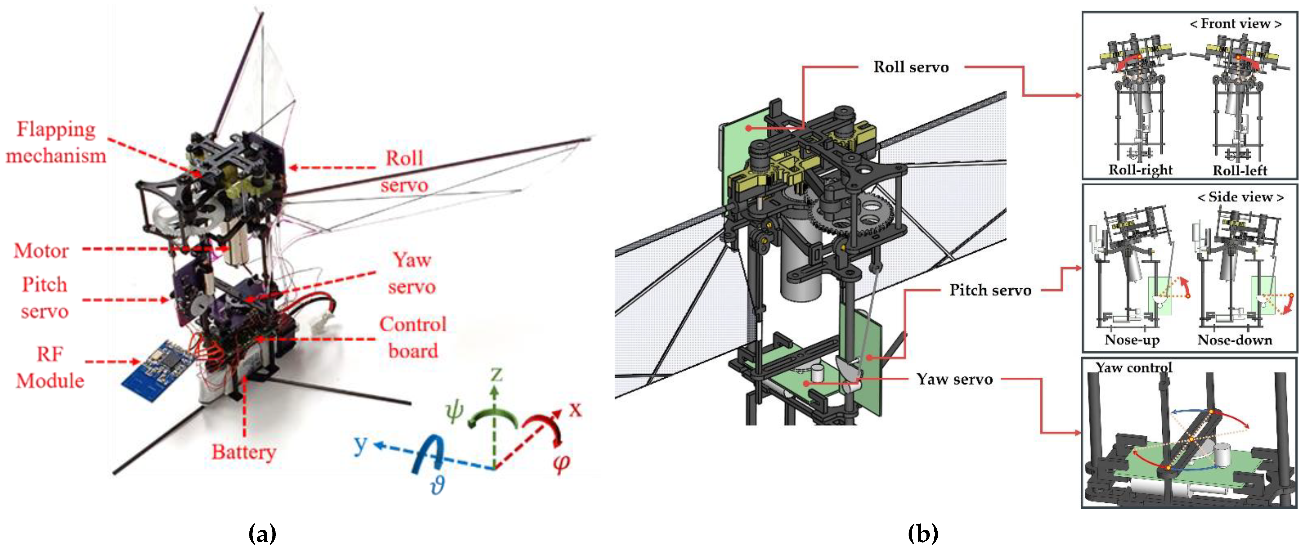
2.1. KUBeetle Design

Figure 1 shows the KUBeetle [30,31,32,33,34,35,83,84], a tailless FWMAV used for parameter identification in this study. The design of the KUBeetle in this study slightly differed from that of a previously developed KUBeetle [34]. They were mainly different in their flapping mechanisms and the location of the control board. One pair of wings of the KUBeetle were modulated by a DC motor using a rack and pinion mechanism to perform a high-amplitude flapping motion for thrust generation [85], whereas previous models used a pulley-string mechanism [30,31]. In the current KUBeetle, the control board was placed between the yaw servo motor and battery, which could lower the center of gravity (CG) position compared with the older version of the KUBeetle. The control board was designed to receive the reference command to control the FWMAV and transmit flight data in real time through a wireless communication RF module extension. A previous study [34] explains the detailed design and specifications of the control board. Figure 1b shows that the flight stability and control are maintained by manipulating the wing stroke plane using three servo motors to generate control moments for pitch, roll, and yaw.

2.2. Dynamic Model

System identification using a gray box model requires an initial dynamic model with starting parameters. The longitudinal mode dynamic model of the KUBeetle used in this study was based on Newton–Euler equations of motion at near-hover conditions [86,87,88,89]. The dynamic model was extended to include filters and servo motor dynamics [34]. Parameters (specifically, the moments of inertia and filter parameters) were updated according to the latest KUBeetle design.

Table 1. Stability and control derivatives.

$X_u$ [${\mathrm{N}\mathrm{s}\mathrm{m}}^{-1}$]	$X_w$ [${\mathrm{N}\mathrm{s}\mathrm{m}}^{-1}$]	$X_q$ [${\mathrm{N}\mathrm{s}\mathrm{rad}}^{-1}$]	$Z_u$ [${\mathrm{N}\mathrm{s}\mathrm{m}}^{-1}$]	$Z_w$ [${\mathrm{N}\mathrm{s}\mathrm{m}}^{-1}$]	$Z_q$ [${\mathrm{N}\mathrm{s}\mathrm{rad}}^{-1}$]
$-2.39\times {10}^{-2}$	$2.79\times {10}^{-4}$	$6.22\times {10}^{-4}$	$1.06\times {10}^{-3}$	$-1.34\times {10}^{-2}$	$1.15\times {10}^{-4}$
$M_u$ [$\mathrm{N}\mathrm{s}$]	$M_w$ [$\mathrm{N}\mathrm{s}$]	$M_q$ [${\mathrm{N}\mathrm{s}\mathrm{m}\mathrm{rad}}^{-1}$]	$X_{\gamma p}$ [${\mathrm{N}\mathrm{rad}}^{-1}$]	$Z_{\gamma p}$ [${\mathrm{N}\mathrm{rad}}^{-1}$]	$M_{\gamma p}$ [${\mathrm{N}\mathrm{m}\mathrm{rad}}^{-1}$]
$-8.3\times {10}^{-4}$	$-1.6\times {10}^{-5}$	$-6.2\times {10}^{-6}$	$1.32\times {10}^{-1}$	$-2.03\times {10}^{-2}$	$1.38\times {10}^{-2}$

shows the stability and control derivatives obtained from the computational fluid dynamics (CFD) analysis and force and moment measurements. Figure 1 shows the body frame of the KUBeetle. The extended longitudinal mode dynamic model is described below [34,86,87,88,89]:

$${\dot{x}}_{ext}=A_{ext} x_{ext}+B_{ext} u_{ext},$$

(1)

$$y_{ext}=C_{ext} x_{ext},$$

(2)

$$x_{ext}=\left[\begin{array}{c}\begin{array}{c}u\\ w\\ q\\ \vartheta \end{array}\\ {\widehat{q}}_{lpf}\\ {\widehat{\vartheta }}_{lpf}\\ {\widehat{\vartheta }}_{kf,angle}\\ {\widehat{\vartheta }}_{kf,bias}\\ u_{servo}\end{array}\right],$$

(3)

where $u$ and $w$ are velocities along the x- and z-axis, respectively; $q$ is the pitch rate (rad/s); $\vartheta$ is the pitch angle (rad); $u_{ext}$ is the control input in the form of pitch servo angle; $y_{ext}$ is the output or response of the KUBeetle; ${\widehat{q}}_{lpf}$ is the low-pass filtered pitch rate; ${\widehat{\vartheta }}_{lpf}$ is the low-pass filtered pitch angle; ${\widehat{\vartheta }}_{kf,angle}$ and ${\widehat{\vartheta }}_{kf,bias}$ are the pitch angle and bias estimation of the Kalman filter, respectively, and $u_{servo}$ is the servo output. The system and input matrices of the extended dynamic model are given below [34,86,87,88,89]:

$$A_{ext}=\left[\begin{array}{ccccccccc}\frac{X_u}{m}& \frac{X_w}{m}& \frac{X_q}{m}& g& 0& 0& 0& 0& \frac{X_{\gamma p}}{m}\\ \frac{Z_u}{m}& \frac{Z_w}{m}& \frac{Z_q}{m}& 0& 0& 0& 0& 0& \frac{Z_{\gamma p}}{m}\\ \frac{M_u}{I_{yy}}& \frac{M_w}{I_{yy}}& \frac{M_q}{I_{yy}}& 0& 0& 0& 0& 0& \frac{M_{\gamma p}}{I_{yy}}\\ 0& 0& 1& 0& 0& 0& 0& 0& 0\\ 0& 0& 204.3& 0& -204.3& 0& 0& 0& 0\\ 0& 0& 0& 10.13& 0& -10.13& 0& 0& 0\\ 0& 0& 0& 0& 1& 0.329& -0.329& 1& 0\\ 0& 0& 0& 0& 0& -0.05& 0.05& 0& 0\\ 0& 0& 0& 0& 0& 0& 0& 0& -30.67\end{array}\right],$$

(4)

$$B_{ext}=\left[\begin{array}{c}0\\ 0\\ 0\\ 0\\ 0\\ 0\\ 0\\ 0\\ 30.91\end{array}\right],$$

(5)

where $X$ and $Z$ are aerodynamic forces along the x- and z-axes, respectively, and $M$ is the aerodynamic pitching moment about the CG. Subscripts $u$, $w$, and $q$ indicate their aerodynamic derivatives with respect to $u$, $w$, and $q$. The subscript $\gamma p$ implies control input by the pitch servo. $m$ is the mass of the KUBeetle ($17.7\times {10}^{-3} \mathrm{kg}$), $I_{yy}$ is the pitching moment of inertia (12.43 $\times {10}^{-6}{\mathrm{kg}\mathrm{m}}^2$), and $g$ is the gravitational acceleration $\left(9.81 {\mathrm{m}\mathrm{s}}^{-2}\right)$. The first four rows of the system matrix consisted of parameters of the basic dynamic model [34]. In the fifth and sixth rows, parameters of low-pass filters for pitch rate and pitch angle were included, respectively. The seventh and eighth rows included Kalman filter parameters for pitch angle and bias estimation. Finally, the last row contained servo motor dynamic parameters. The output matrix of the extended dynamic model, $C_{ext}$ (open-loop) or $C_{ext,cl}$ (closed-loop), can be adjusted according to the number of available outputs for system identification. For pitch angle and pitch rate outputs, the output matrix is given as follows:

$$C_{ext1}=C_{ext,cl1}=\left[\begin{array}{ccccccccc}0& 0& 0& 0& 1& 0& 0& 0& 0\\ 0& 0& 0& 0& 0& 0& 1& 0& 0\end{array}\right].$$

(6)

For pitch angle output only, the output matrix was given as:

$$C_{ext2}=C_{ext,cl2}=\left[\begin{array}{ccccccccc}0& 0& 0& 0& 0& 0& 1& 0& 0\end{array}\right].$$

(7)

In general, it is not feasible or practical to identify an unstable system. Therefore, a simple PD feedback controller was added to the unstable system to obtain a stable closed-loop control system. The same PD gains in a previous study [34] were used as the starting reference. They were then slightly tuned through experimental flight. Figure 2 shows the data acquisition structure of system identification with a PD feedback controller. Pitch rate estimation was obtained after the pitch rate output of the dynamic model was filtered by a low-pass filter [34]. Considering real time implementation, a first order low-pass filter (cutoff frequency 32 Hz) was used to reduce the high-frequency noise because of its simplicity which took a small calculation time and memory of the microprocessor. Pitch angle estimation was obtained by combining low-pass filtered pitch rate output and pitch angle estimated from acceleration outputs using the Kalman filter [34]. The KUBeetle showed stable flight performance with the current filters, especially on hovering, although there were some oscillating motions, indicating that the current setup was sufficient for an experimental flight.

A closed-loop system identification is more challenging than an open-loop system identification due to existing feedback. The feedback can affect system identification performance by making the closed-loop system less sensitive to parameter changes in an open-loop system [79]. In addition, the natural dynamic of the KUBeetle toward the reference command might be regarded as a disturbance that needs to be damped and minimized by the controller [77,78]. However, the feedback also allows for more input in a specific frequency range without increasing the output magnitude [79]. Two different methods [79,82], direct and indirect, were tested to identify the longitudinal mode dynamic model of KUBeetle. According to Figure 2, the direct method used sets of control input and output data to obtain the open-loop dynamic model, while the indirect method used sets of reference command and output data to obtain the closed-loop dynamic model. It is possible to use the indirect approach, because the structure of the state space of the closed-loop extended dynamic model is fully known.

A simple PD controller with reference command is given bellow [34]:

$$u_{pd}=K_P\left({\vartheta }_{ref}-{\widehat{\vartheta }}_{kf,angle}\right)-K_D{\widehat{q}}_{lpf},$$

(8)

where $u_{pd}$ is the control input, ${\vartheta }_{ref}$ is the angle reference command, $K_P$ is the proportional controller gain, and $K_D$ is the derivative controller gain. The system matrix and input matrix of the closed-loop extended dynamic model can be expressed as follows:

$$A_{ext,cl}=\left[\begin{array}{c}{A}_{ext}\left(1:8, 1:9\right)\\ \begin{array}{ccccccccc}0& 0& 0& 0& -30.91K_D& 0& -30.91K_P& 0& -30.67\end{array}\end{array}\right],$$

(9)

$$B_{ext,cl}=\left[\begin{array}{c}{B}_{ext}\left(1:8, 1\right)\\ 30.91K_P\end{array}\right].$$

(10)

The addition of a PD controller to the extended dynamic model only changed the last row of the state space matrix where the control input was given to the servo. Either an open-loop or a closed-loop extended dynamic model could be used as the starting reference in system identification with the gray box model approach. The open-loop extended dynamic model could be retrieved simply by setting controller gain parameters on the last row of the system matrix to zero and changing the last parameter of the input matrix to 30.91, according to Equations (4) and (5). Moreover, it should be noted that velocities along the x- and z-axes were not measured. They could not be used for system identification, which makes the system identification more challenging.

Parameters of the filters, servo motor, and PD controller were fixed, because their values were already known and verified [34]. The gravity, integrator, and zero constants were also fixed. Thus, only nine stability derivatives and three control derivates were refinable in system identification. Each parameter had different physical characteristics and an effect on the dynamic of the KUBeetle [87,88,89]. Based on CFD analysis [89], $X_u$, $Z_w$, and $M_u$ should be negative and have relatively large magnitudes; $X_w$, $Z_u$, $Z_q$, and $M_w$ should be close to zero; and $X_q$ and $M_q$ should have relatively small magnitudes. Overall, $X_u$, $X_q$, $Z_w$, $M_u$, and $M_q$, the five parameters of stability derivatives, and $X_{\gamma p}$, $Z_{\gamma p}$, and $M_{\gamma p}$, the three parameters of control derivatives, were mainly focused on for system identification. During system identification, these eight parameters were refined with a relatively wide range of restriction. Conversely, non-focused parameters of stability derivatives were kept close to zero with a narrow range of restriction. Restrictions were adjusted considering computational fluid dynamics (CFD) results [87,88,89] and current KUBeetle design specifications to maintain the integrity of the identified dynamic model in relation to the physical system. While relaxing parameter restrictions might improve the result of system identification, some refined parameters might not match the real physical system.

3. Experimental Flight and System Identification

In this study, the system identification process was performed in the following steps: (1) experimental flight setup; (2) data acquisition for system identification via experimental flight; (3) linear model refinement in system identification using the gray box model approach; and (4) dynamic model analysis and verification.

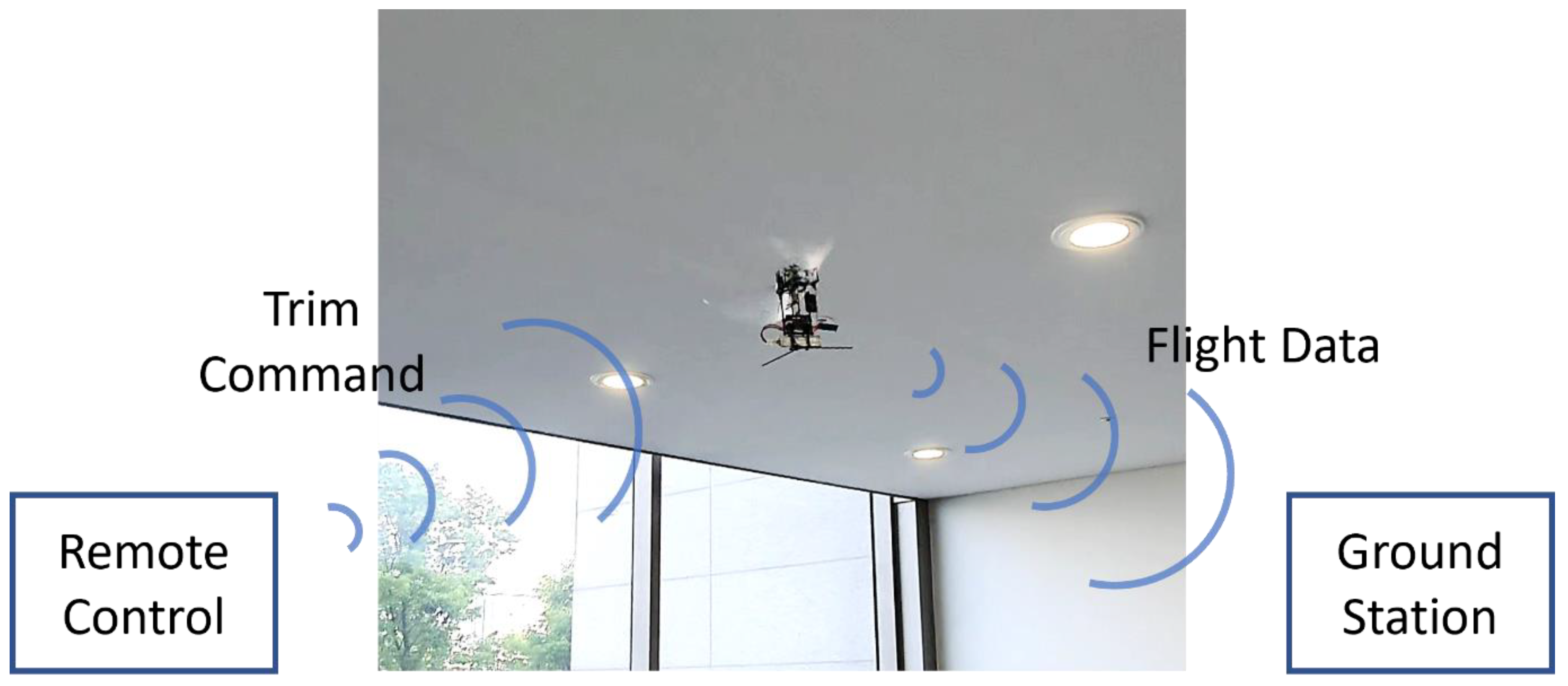
3.1. Experimental Flight Setup

Figure 3 shows the experimental flight setup to obtain flight data for system identification. This setup consisted of a remote control, the KUBeetle, and a ground station. The remote control was used for throttle adjustment for taking off, hovering, and landing the KUBeetle. It was also used for adjusting and maintaining trim conditions during the experimental flight. The flight was conducted indoors without wind disturbance. All experimental flight data were obtained and processed with an onboard control board equipped with an inertial measurement unit (MPU-9250, InvenSense, San Jose, CA, USA). Flight data were then transmitted via wireless communication (NRF24L01+, Nordic Semiconductor, Trondheim, Norway) to the ground station. Considering that the bandwidth of the longitudinal mode dynamics with the PD controller was less than 20 rad/s, the sampling rate was set to be 100 Hz. Recorded data consisted of time, pitch reference command, pitch angle, and pitch rate. In addition, the control input was calculated from the reference command and output data with known control gains.

3.2. Data Acqusition for System Identification via Experimental Flight

Initially, the KUBeetle was manually kept in a hovering condition with minimum drift via a remote control. In hovering condition, the preprogrammed command in the control board was triggered through the remote control to automatically apply reference commands to the KUBeetle. Preprogrammed command was used to ensure the repeatability and consistency during each experimental flight. The reference command is a very important component of the system identification because it affects entire aspects of the system identification process. The reference command should be able to excite as many dynamic modes of interest and natural dynamics as possible to provide comprehensive data for system identification [77,78,79,80]. With the dynamic of the KUBeetle in consideration, two different reference commands were used in the experimental flight. The first reference command was in the form of a regular square signal with a relatively long and constant period (amplitude: ±17° (0.3 rad); period: 6 s) to analyze transient and steady state responses of the KUBeetle (Supplementary Materials Video S1). The second reference command consisted of an irregular square signal with varying periods (amplitude: ±17° (0.3 rad); period: 0.2 to 1.4 s) to cover the frequency bandwidth of interest (Supplementary Materials Video S2). The second reference command was generated using a pseudo-random binary signal, which was a periodic and deterministic signal with properties such as white noise [79]. The amplitude and period of the reference command were chosen considering the operating range of the KUBeetle. Assuming the same amplitude and frequency range, the square signal covered a similar range to that of a chirp signal, as indicated by the frequency spectrum of reference commands shown in Figure 4:

For clarity, the extended dynamic model with parameters obtained from CFD and force and moment measurements, later used as the initial dynamic model in system identification, is called the CFD dynamic model. Figure 5 shows experimental and simulation results of the KUBeetle with a regular square command for pitch. Together with the preprogrammed command, the constant trim control input from the remote control was applied to the KUBeetle. The constant trim command was subtracted to obtain the reference command from the actual command input applied. Small noises were added while the trim control input was being read from the pulse-width-modulated signal. The reference command was the summation of the preprogrammed command and the added trim command noise. Figure 5a shows that the closed-loop KUBeetle has a relatively slow response, high overshoot, and large steady state error. After the reference command was provided, the KUBeetle attempted to follow the reference command in the beginning by responding quickly according to the stroke plane change via the servo motor. However, it was gradually stabilized to a low pitching angle, which maintained the large steady state error. This phenomenon was mainly caused by the position of the CG that affected the force and the moment generated by the gravity force during flight. The CG was located at a relatively large distance below the aerodynamic center (AC). Figure 5b presents the pitch rate responses to a regular square reference command, showing that the measured pitch rate still had a large periodic and high-frequency noise due to wing flapping.

Figure 6 demonstrates experimental and simulation results of the KUBeetle with an irregular square reference command. Figure 6a shows the pitch angle responses. In some intervals, the pitch angle response misleadingly looks as if it is following the command signal well, although some phase delays exist. This is due to overshooting responses at the beginning of step inputs. However, as the frequency of the reference command increased, it could not follow the reference command. Figure 6b illustrates that the pitch rate was contaminated with large noise, as in the regular square reference command case shown in Figure 5b. The high-frequency noise was still very large on the angular rate signal, although it was low-pass filtered (cutoff frequency 32 Hz). However, it was not easy to remove it without invoking much phase delay, which degraded the closed-loop stability. Thus, the current setup was kept for the experimental flight.

3.3. Linear Model Refinement in System Identification

System identification processes were performed with the help of system identification tools in MATLAB^®. The dynamic model generated from the system identification using the black box model approach was found to be very complex. It could not be matched with real physical parameters of the KUBeetle. Thus, this research only focused on the system identification using the gray box model approach. The gray box model approach with direct and indirect methods was tested to refine open- and closed-loop dynamic models. Two different pairings were considered for the direct and indirect methods, respectively. Firstly, the control input was given as input, while the pitch rate and pitch angle were given as outputs. Secondly, the reference command was given as input, while the pitch rate and pitch angle were given as outputs. Equations (4) and (5) present the structure of the system and input matrices of the dynamic model as fixed for the open-loop dynamic model, while Equations (9) and (10) present those for the closed-loop dynamic model. In addition, given values of parameters in Equations (4)–(10), obtained from computations and measurements, were used as the initial values for system identification. The pitch angle output was given higher weighting, because it had smaller noise compared to the pitch rate output which had larger high-frequency noise that could affect the accuracy of the identified dynamic model. According to the experimental flight setup and data, the obtained dynamic model mainly represented the dynamic of KUBeetle during hover and forward flights with pitch angle under 0.3 radian. Adaptive Gauss–Newton (GNA), Levenberg–Marquardt (LM), and gradient search (GRAD) methods were utilized for model refinements.

Table 2. General characteristics of each identification method.

Identification Method	Characteristics
GNA	The adaptive subspace Gauss–Newton search method.
	This minimizes the objective function, which is the sum of squared errors that is approximately quadratic in the parameters near the optimal solution.
	Convergence is not guaranteed, and it might converge only to a local optimum, depending on the starting parameters.
LM	The Levenberg–Marquardt least square search method.
	This updates the parameters by adaptively combining the Gauss–Newton and gradient descent approaches, depending on the parameter errors.
	This is a refinement to the Gauss–Newton search method that improves the chance of local convergence and prevents divergence.
	This method is more robust than the Gauss–Newton and gradient descent search methods.
GRAD	The Steepest descent or Gradient descent search method.
	This updates the parameters towards the largest directional derivative or negative gradient direction of the objective function to reduce the sum of squared errors.
	When close to minimum, the iteration process becomes relatively slow.

summarizes the general characteristics of each identification method [90,91,92]:

The total iteration for each search method was limited to 2000 iterations, as further iterations provided negligible improvement. Results from each search method were compared and evaluated. One of the indicators used was the fit percentage of the responses of the identified dynamic model to the experimental flight data. It was defined as:

$$Fit Percentage=100\left(1-\frac{\sqrt{{\sum }_{i=1}^N{\left(y_{measured}-y_{model}\right)}^2}}{\sqrt{{\sum }_{i=1}^N{\left(y_{measured}-\overline{y_{measured}}\right)}^2}}\right),$$

(11)

where, $N$ was the number of samples, $y_{measured}$ was the experimental flight data measured, $y_{model}$ was the simulated response of the dynamic model identified, and $\overline{y_{measured}}$ was the mean of experimental flight data measured.

Firstly, system identification using the gray box model approach with the direct method was conducted. Closed-loop system identification with the direct method is often used, because it works regardless of the complexity of the regulator. In addition, it does not require knowledge of the characteristic of the feedback [79]. However, the system identification result depended on the quality of the disturbance model, which should also be identified during model refinement. The open-loop CFD dynamic model in Equations (4) and (5) was used as the initial dynamic model. However, the direct method was found to be unsuitable for the system identification of the KUBeetle using the current experimental flight data as the disturbance model could not be identified well, which caused responses of the identified model not to match experimental flight data. Note that some working identification methods for open-loop system identification may fail when they are applied to a closed-loop system identification [79].

Secondly, considering that the open-loop dynamic model could easily be retrieved from the closed-loop dynamic model, system identification using the gray box model approach with the indirect method was conducted. In the indirect method, the system matrix of the closed-loop CFD dynamic model in Equations (9) and (10) was used as the initial dynamic model. Through system identification with several different methods and various restriction settings, several identified dynamic models were obtained. The criteria to select the identified dynamic model were: (1) the fit percentage should be high enough; (2) time-domain responses of the closed-loop dynamic model should have similar characteristics to the experimental flight data; and (3) the open-loop dynamic model should have similar stable and unstable poles and zeros to those of the computationally calculated dynamic model, whereas the closed-loop dynamic model with the PD feedback controller should be stable.

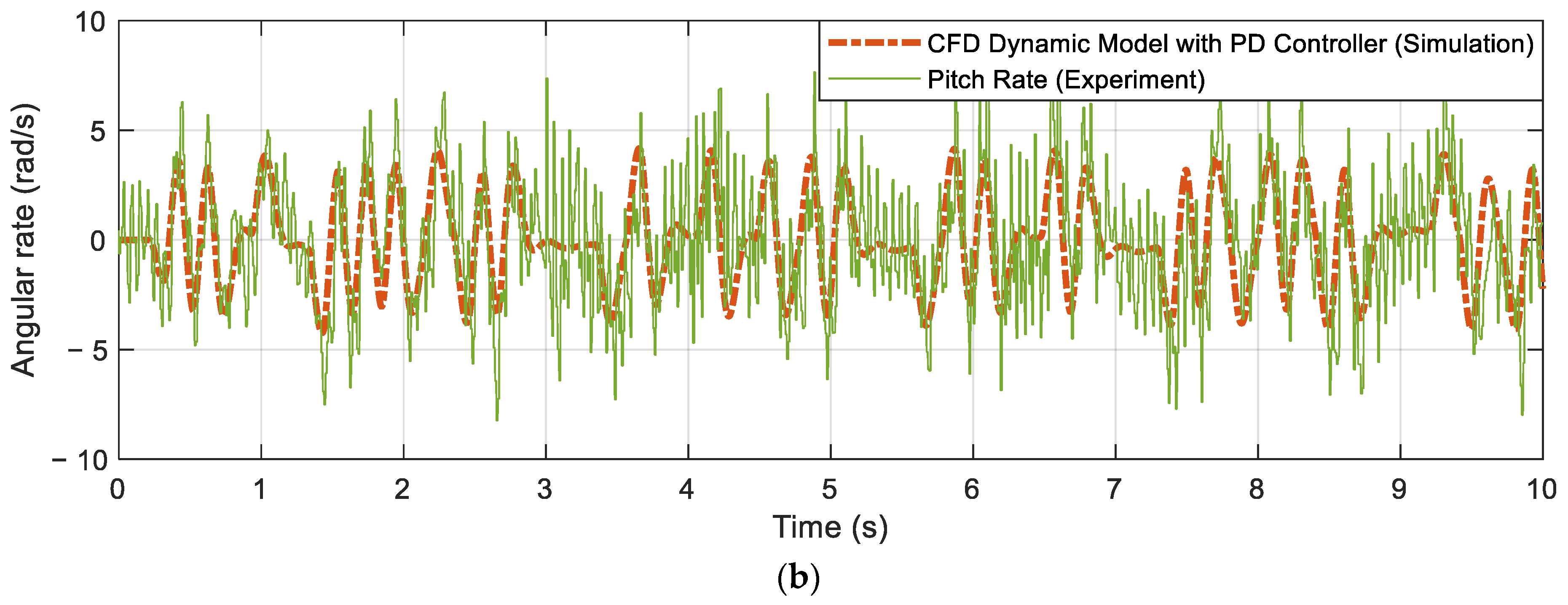
3.4. Dynamic Model Analysis and Verification

Single or a combination of multiple sets of experimental flight data were tested to obtain the best identified dynamic model. This was completed to evaluate the consistency of the identification results and sensitivity of the identification methods. It was found that identified parameters related to velocities along the x- and z-axes had relatively larger deviations because they were not available using onboard sensors. In addition, high-frequency noises and nonlinear body dynamics not included in the model also affected identification results. By following all the selection criteria, six identified dynamic models were considered.

Table 3. Refined parameters of identified dynamic models using an indirect method.

Parameters	CFD (Initial)	Identified Dynamic Model
		GNA 1	LM 1	GRAD 1	GNA 2	LM 2	GRAD 2	Average
$X_u/m$	−1.351	0.000	0.000	0.000	0.000	0.000	0.000	0.000
$Z_u/m$	0.060	0.001	0.000	0.000	0.000	0.028	0.000	0.005
$M_u/I_{yy}$	−66.755	−79.656	−79.870	−75.722	−87.300	−99.508	−83.732	−84.298
$X_w/m$	0.016	4.237	4.237	4.237	4.237	4.237	4.237	4.237
$Z_w/m$	−0.756	−1.464	−1.742	−1.645	−1.268	−1.113	−1.646	−1.480
$M_w/I_{yy}$	−1.287	−1.126	−1.126	−1.126	−1.126	−1.227	−1.126	−1.143
$X_q/m$	0.035	0.294	0.560	0.347	−0.044	−0.058	−0.002	0.183
$Z_q/m$	0.006	0.006	0.006	0.006	0.006	0.006	0.006	0.006
$M_q/I_{yy}$	−0.499	−7.715	−1.532	−3.622	−6.470	−7.467	−4.460	−5.211
$X_{\gamma p}/m$	7.458	16.553	20.746	21.329	12.767	9.796	18.457	16.608
$Z_{\gamma p}/m$	−1.147	−11.333	−14.579	−14.826	−8.953	−7.405	−13.671	−11.795
$M_{\gamma p}/I_{yy}$	1109.171	1015.702	1092.554	1108.319	1016.950	1058.045	1107.437	1066.501
Fit Percentage	21.982	49.090	48.640	49.920	45.110	43.180	46.520	48.300

shows parameters of the identified dynamic model with the indirect method. Each of the selected dynamic models was named based on the identification method used to refine it and numbers represent datasets used for the identification. Fit percentages of identified models obtained using irregular and high-frequency reference signals were much lower than those obtained using regular and low-frequency reference signals. Thus, they were discarded. The fit percentage of the dynamic model from CFD was only about 22%. This low fit percentage was mainly because only wing parts were considered to obtain the stability derivative-related parameters, instead of using the whole body of the KUBeetle. The whole body of the KUBeetle, including the wings, was considered to obtain mass and moments of inertia. The average fit percentage of the identified dynamic models was approximately 49%, which was more than double that of the CFD dynamic model. Most parameter values obtained from the three different identification methods and CFD were quite similar to each other. The CG of the new KUBeetle design, being lower than the CG of the previous KUBeetle design, increased the magnitude of $M_u$. This was in accordance with the shift of the CG position due to the relocation of the control board and RF module from the top of the flapping mechanism to under the motor. The increase in $M_q$ showed that the system had higher damping than that initially given from CFD. This indicated that the body of the KUBeetle greatly affected system stability. According to system identification results, aerodynamic forces along the x- and z-axes, $X_{\gamma p}$ and $Z_{\gamma p}$, had larger magnitudes than that previously measured. When measuring the control derivative, only the wings and frames near the wing were included. Because of a mounting problem, the lower body of the KUBeetle could not be included, which could be one of the possible reasons for the difference. Other parameters maintained similar values to CFD values.

Using the current flight data and dynamic model structure, it was not easy to obtain dynamic model parameters with high fit percentage, even using the black box model approach where there were no parameter restrictions. Moreover, it was found that the parameters obtained were a little sensitive to the datasets used for system identification. The possible reasons for this were: (1) velocities along x- and z-axes were not measured, which degraded the accuracy of the related parameters, $X_u$, $X_w$, $X_q$, $Z_u$, $Z_w$, and $Z_q$; (2) high-frequency noise also contributed to accuracy degradation; and (3) there were nonlinear coupling dynamic terms not included in the model. It has been reported that accuracy can be improved if velocities along the x- and z-axes are available and nonlinear coupling terms are included [77].

Although all dynamic model candidates showed similar fit percentages, GRAD1 was chosen for analysis and evaluation since it had the highest fit percentage. Identified parameters were evaluated in the basic form of the dynamic model [34], where filters and servo dynamics were not included. The basic dynamic model is described as follows:

$${\dot{x}}_{basic}=A_{basic} x_{basic}+B_{basic} u_{basic},$$

(12)

$$y_{basic}=C_{basic} x_{basic},$$

(13)

$$x_{basic}=\left[\begin{array}{c}\begin{array}{c}u\\ w\\ q\\ \vartheta \end{array}\end{array}\right],$$

(14)

$$A_{basic}=\left[\begin{array}{cccc}\frac{X_u}{m}& \frac{X_w}{m}& \frac{X_q}{m}& g\\ \frac{Z_u}{m}& \frac{Z_w}{m}& \frac{Z_q}{m}& 0\\ \frac{M_u}{I_{yy}}& \frac{M_w}{I_{yy}}& \frac{M_q}{I_{yy}}& 0\\ 0& 0& 1& 0\end{array}\right],$$

(15)

$$B_{basic}=\left[\begin{array}{c}\frac{X_{\gamma p}}{m}\\ \frac{Z_{\gamma p}}{m}\\ \frac{M_{\gamma p}}{I_{yy}}\\ 0\end{array}\right],$$

(16)

and $C_{basic}$ was set as $\left[\begin{array}{cc}0& \begin{array}{ccc}0& 0& 1\end{array}\end{array}\right]$ to describe the pitch angle measurement.

Figure 7 shows the open-loop frequency responses and a Nyquist diagram of the GRAD1 and CFD dynamic models. When the frequency was under 0.01 rad/s, the low-frequency gain of the identified GRAD1 dynamic model was similar to that of the CFD dynamic model. As the frequency increased to higher than 0.3 rad/s, the gain of the GRAD1 dynamic model was smaller than that of the CFD dynamic model. Moreover, at mid-frequency, the GRAD1 dynamic model had a local minimum point. As the frequency further increased to higher than 5 rad/s, both dynamic models had similar characteristics. Poles of the GRAD1 were (2.86 ± 8.46i, −9.35, −1.64), while those of the CFD model were (3.69 ± 7.58i, −9.22, −0.76). The unstable pole locations did not move much. However, the magnitude of the stable dominant pole of the GRAD1 dynamic model was larger than that of the CFD dynamic model. Thus, it is expected that response of the GRAD1 dynamic model is faster than that of the CFD dynamic model. Both basic dynamic models encircle the (−1, 0) point two times in the Nyquist diagram, meaning that if the loop is closed, the two systems will be stable. However, Figure 7b shows that both models have very small phase margins, with less than 8 degrees.

The simulation was used to analyze and compare extended dynamic models as shown in Figure 8. Gain and phase margins of the GRAD1 dynamic model were 17.2 dB and 39.0°, respectively, while the gain and phase margins of the CFD dynamic model were 16.5 dB and 30.3°, respectively. In the Nyquist diagram, both extended dynamic models encircled the (−1, 0) point two times. Both dynamic models had small gains in the low-frequency range, which resulted in a large steady state error. To reduce the steady state error, the loop gain should be increased. However, this may decrease the stability margins.

Figure 9 shows experimental flight data and simulation results of the GRAD1 dynamic model using the PD feedback controller. As shown in Figure 9a, the pitch angle response of the GRAD1 dynamic model was closer to the pitch angle from the experimental flight data compared to that of the dynamic model from CFD. The peak and valley points predicted using the GRAD1 dynamic model were more accurate than those of the CFD dynamic model. Figure 9b also shows that the GRAD1 dynamic model was better than the CFD dynamic model in following the pitch rate from the experimental flight data, neglecting the high-frequency noise. The high-frequency noise was due to wing flapping, which degraded the performances of system identification and control.

4. Conclusions

In this study, we identified a dynamic model of the KUBeetle with several identification approaches and methodologies using angle and angular rate data from onboard sensors only. The gray box model approach was preferred to the black box model approach, because the structure and integrity of parameters of the dynamic model could be maintained. Higher weighting was given to the angle output because it had much lower noises compared to angular rate output. It was found that dynamic models with high fit percentage were obtained using datasets which included the data obtained using regular and low-frequency reference commands. In addition, obtained parameters were slightly sensitive to the quality of the dataset. GNA, LM, and GRAD identification methods showed similar results to each other for two different datasets, while GRAD1 showed the highest fit percentage. These consistent results indicate that the dynamic model was quite reliable and could represent the main dynamic of the KUBeetle, although nonlinear dynamics were not fully identified. Compared to that of the CFD dynamic model, the fit percentage was improved from 22% to 49%. Increases in $M_u$ complied with the lower CG of the KUBeetle. In addition, the increases in $M_q$ indicated higher damping caused by the body dynamics of the KUBeetle that were not considered previously. The obtained dynamic model mainly works for predicting hover and forward flight responses with pitch angle reference command under 0.3 radian, which is used in an experimental flight. The obtained dynamic model described the pitch angular motion quite well, while the linear velocity-related parameters needed more improvement. This is because there was no onboard speed sensor.

From frequency domain analysis, it was found that the open-loop GRAD1 model had a small phase margin indicating that KUBeetle stability could be easily affected by the angular rate feedback gain changes. Moreover, the GRAD1 dynamic model had a faster response because its stable dominant pole had a larger magnitude than the CFD dynamic model. In addition, it showed a similar response to the experimental flight data, neglecting high-frequency noises. It is expected that if the high-frequency noise due to flapping could be reduced and the velocity could be estimated, the fit percentage could be further improved. The time-domain and frequency responses of the identified dynamic model were considerably closer to experimental flight data than those obtained by numerical computation. Further studies are needed to reduce the high-frequency noise due to flapping, to better estimate forward and vertical velocities, and to improve the accuracy of identification.

References

1. Sanchez, C.; Arribart, H.; Giraud Guille, M.M. Biomimetism and Bioinspiration as Tools for the Design of Innovative Materials and Systems. Nat. Mater. 2005, 4, 277–288. [Google Scholar] [CrossRef] [PubMed]
2. Tan, R.; Liu, W.; Cao, G.; Shi, Y. Creative Design Inspired by Biological Knowledge: Technologies and Methods. Front. Mech. Eng. 2019, 14, 1–14. [Google Scholar] [CrossRef] [Green Version]
3. Fukuda, T.; Chen, F.; Shi, Q. Special Feature on Bio-Inspired Robotics. Appl. Sci. 2018, 8, 817. [Google Scholar] [CrossRef] [Green Version]
4. Wang, J.; Chen, W.; Xiao, X.; Xu, Y.; Li, C.; Jia, X.; Meng, M.Q.-H. A Survey of the Development of Biomimetic Intelligence and Robotics. Biomim. Intell. Robot. 2021, 1, 100001. [Google Scholar] [CrossRef]
5. Biswal, P.; Mohanty, P.K. Development of Quadruped Walking Robots: A Review. Ain Shams Eng. J. 2021, 12, 2017–2031. [Google Scholar] [CrossRef]
6. Zhu, H.; Gu, S.; He, L.; Guan, Y.; Zhang, H. Transition Analysis and Its Application to Global Path Determination for a Biped Climbing Robot. Appl. Sci. 2018, 8, 122. [Google Scholar] [CrossRef] [Green Version]
7. Liljebäck, P.; Pettersen, K.Y.; Stavdahl, Ø.; Gravdahl, J.T. A Review on Modelling, Implementation, and Control of Snake Robots. Robot. Auton. Syst. 2012, 60, 29–40. [Google Scholar] [CrossRef] [Green Version]
8. Razif, M.; Mohd Faudzi, A.A.; Mohd Nordin, I.N.A.; Natarajan, E.; Yaakob, O. A Review on Development of Robotic Fish. J. Transp. Syst. Eng. 2014, 1, 12–22. [Google Scholar]
9. Duraisamy, P.; Kumar Sidharthan, R.; Nagarajan Santhanakrishnan, M. Design, Modeling, and Control of Biomimetic Fish Robot: A Review. J. Bionic Eng. 2019, 16, 967–993. [Google Scholar] [CrossRef]
10. A Robot That Flies like a Bat. Nature 2017, 542, 140. [CrossRef] [Green Version]
11. Bie, D.; Li, D.; Xiang, J.; Li, H.; Kan, Z.; Sun, Y. Design, Aerodynamic Analysis and Test Flight of a Bat-Inspired Tailless Flapping Wing Unmanned Aerial Vehicle. Aerosp. Sci. Technol. 2021, 112, 106557. [Google Scholar] [CrossRef]
12. Han, J.-H.; Lee, J.-S.; Kim, D.-K. Bio-Inspired Flapping UAV Design: A University Perspective. In Health Monitoring of Structural and Biological Systems 2009; Kundu, T., Ed.; SPIE: Bellingham, WA, USA, 2009; pp. 466–477. [Google Scholar]
13. Tan, X.; Zhang, W.; Ke, X.; Chen, W.; Zou, C.; Liu, W.; Cui, F.; Wu, X.; Li, H. Development of Flapping-Wing Micro Air Vehicle in Asia. In Proceedings of the 10th IEEE World Congress on Intelligent Control and Automation, Beijing, China, 6–8 July 2012; IEEE: Piscataway, NJ, USA, 2012; pp. 3939–3942. [Google Scholar]
14. Mwongera, V.M. A Review of Flapping Wing MAV Modelling. Int. J. Aeronaut. Aerosp. Res. 2015, 2, 27–36. [Google Scholar] [CrossRef]
15. Unver, O.; Uneri, A.; Aydemir, A.; Sitti, M. Geckobot: A Gecko Inspired Climbing Robot Using Elastomer Adhesives. In Proceedings of the 2006 IEEE International Conference on Robotics and Automation, ICRA 2006, Orlando, FL, USA, 15–19 May 2006; IEEE: Piscataway, NJ, USA, 2006; pp. 2329–2335. [Google Scholar]
16. Nansai, S.; Mohan, R. A Survey of Wall Climbing Robots: Recent Advances and Challenges. Robotics 2016, 5, 14. [Google Scholar] [CrossRef] [Green Version]
17. Sanfilippo, F.; Azpiazu, J.; Marafioti, G.; Transeth, A.; Stavdahl, Ø.; Liljebäck, P. Perception-Driven Obstacle-Aided Locomotion for Snake Robots: The State of the Art, Challenges and Possibilities. Appl. Sci. 2017, 7, 336. [Google Scholar] [CrossRef]
18. Ward, T.A.; Fearday, C.J.; Salami, E.; Binti Soin, N. A Bibliometric Review of Progress in Micro Air Vehicle Research. Int. J. Micro Air Veh. 2017, 9, 146–165. [Google Scholar] [CrossRef]
19. Phan, H.V.; Park, H.C. Insect-Inspired, Tailless, Hover-Capable Flapping-Wing Robots: Recent Progress, Challenges, and Future Directions. Prog. Aerosp. Sci. 2019, 111, 100573. [Google Scholar] [CrossRef]
20. Park, H.C.; Vu, P.H.; Lee, J.H. Tailless Insect-Mimicking Flapping-Wing Micro Air Vehicle: A Review and Perspective. J. ICROS 2019, 25, 960–965. [Google Scholar] [CrossRef]
21. Gerdes, J.W.; Gupta, S.K.; Wilkerson, S.A. A Review of Bird-Inspired Flapping Wing Miniature Air Vehicle Designs. J. Mech. Robot. 2012, 4, 021003. [Google Scholar] [CrossRef] [Green Version]
22. Taylor, G.K. Mechanics and Aerodynamics of Insect Flight Control. Biol. Rev. 2001, 76, 449–471. [Google Scholar] [CrossRef]
23. Dudley, R. The Biomechanics of Insect Flight: Form, Function, Evolution; Princeton Paperbacks; Princeton University Press: Princeton, NJ, USA, 2002; ISBN 978-0-691-09491-5. [Google Scholar]
24. Alexander, D.E. Nature’s Flyers: Birds, Insects, and the Biomechanics of Flight; Johns Hopkins University Press: Baltimore, MD, USA, 2004; ISBN 978-0-8018-8059-9. [Google Scholar]
25. Sun, M. Insect Flight Dynamics: Stability and Control. Rev. Mod. Phys. 2014, 86, 615–646. [Google Scholar] [CrossRef]
26. Zhang, C.; Rossi, C. A Review of Compliant Transmission Mechanisms for Bio-Inspired Flapping-Wing Micro Air Vehicles. Bioinspir. Biomim. 2017, 12, 025005. [Google Scholar] [CrossRef] [PubMed]
27. Keennon, M.; Klingebiel, K.; Won, H. Development of the Nano Hummingbird: A Tailless Flapping Wing Micro Air Vehicle. In Proceedings of the 50th AIAA Aerospace Sciences Meeting including the New Horizons Forum and Aerospace Exposition, Nashville, TN, USA, 9–12 January 2012; American Institute of Aeronautics and Astronautics: Nashville, TN, USA, 2012. [Google Scholar]
28. Ma, K.Y.; Chirarattananon, P.; Fuller, S.B.; Wood, R.J. Controlled Flight of a Biologically Inspired, Insect-Scale Robot. Science 2013, 340, 603–607. [Google Scholar] [CrossRef] [PubMed] [Green Version]
29. Karásek, M.; Muijres, F.T.; De Wagter, C.; Remes, B.D.W.; de Croon, G.C.H.E. A Tailless Aerial Robotic Flapper Reveals That Flies Use Torque Coupling in Rapid Banked Turns. Science 2018, 361, 1089–1094. [Google Scholar] [CrossRef] [PubMed] [Green Version]
30. Phan, H.V.; Kang, T.; Park, H.C. Design and Stable Flight of a 21 g Insect-like Tailless Flapping Wing Micro Air Vehicle with Angular Rates Feedback Control. Bioinspir. Biomim. 2017, 12, 036006. [Google Scholar] [CrossRef]
31. Phan, H.V.; Aurecianus, S.; Kang, T.; Park, H.C. KUBeetle-S: An Insect-like, Tailless, Hover-Capable Robot That Can Fly with a Low-Torque Control Mechanism. Int. J. Micro Air Veh. 2019, 11, 175682931986137. [Google Scholar] [CrossRef] [Green Version]
32. Aurecianus, S.; Na, Y.S.; Vu, P.H.; Park, H.C.; Kang, T. Study of Gyroscope and Accelerometer Dynamic Characteristics on Flapping Wing Micro Aerial Vehicle. J. ICROS 2019, 25, 981–990. [Google Scholar] [CrossRef]
33. Phan, H.V.; Park, H.C. Mechanisms of Collision Recovery in Flying Beetles and Flapping-Wing Robots. Science 2020, 370, 1214–1219. [Google Scholar] [CrossRef]
34. Aurecianus, S.; Phan, H.V.; Kang, T.; Park, H.C. Longitudinal Mode Model-Based Controller Design for Tailless Flapping Wing Robot with Loop Shaping Compensator. Bioinspir. Biomim. 2020, 15, 056004. [Google Scholar] [CrossRef]
35. Aurecianus, S.; Phan, H.V.; Park, J.; Park, H.C.; Kang, T. Lateral Mode Controller Design for Insect-like Tailless Flapping-Wing Micro Air Vehicle. J. ICROS 2021, 27, 1–10. [Google Scholar] [CrossRef]
36. Coleman, D.A.; Benedict, M.; Amp, T.A.; Hrishikeshavan, V.; Chopra, I. Design, Development and Flight-Testing of a Robotic Hummingbird. In Proceedings of the AHS 71st Annual Forum, Virginia Beach, VA, USA, 5–7 May 2015. [Google Scholar]
37. Roshanbin, A.; Altartouri, H.; Karásek, M.; Preumont, A. COLIBRI: A Hovering Flapping Twin-Wing Robot. Int. J. Micro Air Veh. 2017, 9, 270–282. [Google Scholar] [CrossRef] [Green Version]
38. Nguyen, Q.-V.; Chan, W.L. Development and Flight Performance of a Biologically-Inspired Tailless Flapping-Wing Micro Air Vehicle with Wing Stroke Plane Modulation. Bioinspir. Biomim. 2018, 14, 016015. [Google Scholar] [CrossRef] [PubMed]
39. Tu, Z.; Fei, F.; Deng, X. Untethered Flight of an At-Scale Dual-Motor Hummingbird Robot with Bio-Inspired Decoupled Wings. IEEE Robot. Autom. Lett. 2020, 5, 4194–4201. [Google Scholar] [CrossRef]
40. Keennon, M.; Grasmeyer, J. Development of Two MAVs and Vision of the Future of MAV Design. In Proceedings of the AIAA International Air and Space Symposium and Exposition: The Next 100 Years, Dayton, OH, USA, 14–17 July 2003; American Institute of Aeronautics and Astronautics: Dayton, OH, USA, 2003. [Google Scholar]
41. Karásek, M.; Percin, M.; Cunis, T.; van Oudheusden, B.W.; De Wagter, C.; Remes, B.D.; de Croon, G.C. Accurate Position Control of a Flapping-Wing Robot Enabling Free-Flight Flow Visualisation in a Wind Tunnel. Int. J. Micro Air Veh. 2019, 11, 175682931983368. [Google Scholar] [CrossRef] [Green Version]
42. Nguyen, Q.; Chan, W.-L.; Debiasi, M. Performance Tests of a Hovering Flapping Wing Micro Air Vehicle with Double Wing Clap-and-Fling Mechanism. In Proceedings of the International Micro Air Vehicles Conference and Flight Competition, Aachen, Germany, 15–18 September 2015. [Google Scholar]
43. Park, J.H.; Yoon, K.-J. Designing a Biomimetic Ornithopter Capable of Sustained and Controlled Flight. J. Bionic Eng. 2008, 5, 39–47. [Google Scholar] [CrossRef]
44. Rose, C.; Fearing, R.S. Comparison of Ornithopter Wind Tunnel Force Measurements with Free Flight. In Proceedings of the 2014 IEEE International Conference on Robotics and Automation (ICRA), Hong Kong, China, 31 May–7 June 2014; IEEE: Piscataway, NJ, USA, 2014; pp. 1816–1821. [Google Scholar]
45. Folkertsma, G.A.; Straatman, W.; Nijenhuis, N.; Venner, C.H.; Stramigioli, S. Robird: A Robotic Bird of Prey. IEEE Robot. Automat. Mag. 2017, 24, 22–29. [Google Scholar] [CrossRef]
46. Taylor, G.K.; Thomas, A.L.R. Animal Flight Dynamics II. Longitudinal Stability in Flapping Flight. J. Theor. Biol. 2002, 214, 351–370. [Google Scholar] [CrossRef]
47. Taha, H.E.; Kiani, M.; Hedrick, T.L.; Greeter, J.S.M. Vibrational Control: A Hidden Stabilization Mechanism in Insect Flight. Sci. Robot. 2020, 5, eabb1502. [Google Scholar] [CrossRef]
48. Benrabah, M.; Kara, K.; AitSahed, O.; Hadjili, M.L. Adaptive Fourier Series Neural Network PID Controller. Int. J. Control Autom. Syst. 2021, 19, 3388–3399. [Google Scholar] [CrossRef]
49. Freire, H.; Moura Oliveira, P.B.; Solteiro Pires, E.J. From Single to Many-Objective PID Controller Design Using Particle Swarm Optimization. Int. J. Control Autom. Syst. 2017, 15, 918–932. [Google Scholar] [CrossRef]
50. Du, H.; Hu, X.; Ma, C. Dominant Pole Placement with Modified PID Controllers. Int. J. Control Autom. Syst. 2019, 17, 2833–2838. [Google Scholar] [CrossRef]
51. Memon, F.; Shao, C. An Optimal Approach to Online Tuning Method for PID Type Iterative Learning Control. Int. J. Control Autom. Syst. 2020, 18, 1926–1935. [Google Scholar] [CrossRef]
52. Pongfai, J.; Angeli, C.; Shi, P.; Su, X.; Assawinchaichote, W. Optimal PID Controller Autotuning Design for MIMO Nonlinear Systems Based on the Adaptive SLP Algorithm. Int. J. Control Autom. Syst. 2021, 19, 392–403. [Google Scholar] [CrossRef]
53. Fadaei, A.; Salahshoor, K. A Novel Real-Time Fuzzy Adaptive Auto-Tuning Scheme for Cascade PID Controllers. Int. J. Control Autom. Syst. 2011, 9, 823–833. [Google Scholar] [CrossRef]
54. Nguyen, A.T.; Han, J.-H. Wing Flexibility Effects on the Flight Performance of an Insect-like Flapping-Wing Micro-Air Vehicle. Aerosp. Sci. Technol. 2018, 79, 468–481. [Google Scholar] [CrossRef]
55. Nguyen, K.; Au, L.T.K.; Phan, H.-V.; Park, S.H.; Park, H.C. Effects of Wing Kinematics, Corrugation, and Clap-and-Fling on Aerodynamic Efficiency of a Hovering Insect-Inspired Flapping-Wing Micro Air Vehicle. Aerosp. Sci. Technol. 2021, 118, 106990. [Google Scholar] [CrossRef]
56. Nan, Y.; Peng, B.; Chen, Y.; Feng, Z.; McGlinchey, D. Can Scalable Design of Wings for Flapping Wing Micro Air Vehicle Be Inspired by Natural Flyers? Int. J. Aerosp. Eng. 2018, 2018, 9538328. [Google Scholar] [CrossRef]
57. Nan, Y.; Karásek, M.; Lalami, M.E.; Preumont, A. Experimental Optimization of Wing Shape for a Hummingbird-like Flapping Wing Micro Air Vehicle. Bioinspir. Biomim. 2017, 12, 026010. [Google Scholar] [CrossRef] [PubMed]
58. Taha, H.E.; Hajj, M.R.; Nayfeh, A.H. Flight Dynamics and Control of Flapping-Wing MAVs: A Review. Nonlinear Dyn. 2012, 70, 907–939. [Google Scholar] [CrossRef]
59. Orlowski, C.T.; Girard, A.R. Dynamics, Stability, and Control Analyses of Flapping Wing Micro-Air Vehicles. Prog. Aerosp. Sci. 2012, 51, 18–30. [Google Scholar] [CrossRef]
60. Khan, Q.; Akmeliawati, R. Review on System Identification and Mathematical Modeling of Flapping Wing Micro-Aerial Vehicles. Appl. Sci. 2021, 11, 1546. [Google Scholar] [CrossRef]
61. Kajak, K.M.; Karásek, M.; Chu, Q.P.; de Croon, G.C.H.E. A Minimal Longitudinal Dynamic Model of a Tailless Flapping Wing Robot for Control Design. Bioinspir. Biomim. 2019, 14, 046008. [Google Scholar] [CrossRef] [PubMed]
62. Deng, X.; Schenato, L.; Sastry, S.S. Flapping Flight for Biomimetic Robotic Insects: Part II-Flight Control Design. IEEE Trans. Robot. 2006, 22, 789–803. [Google Scholar] [CrossRef]
63. Rifaï, H.; Marchand, N.; Poulin-Vittrant, G. Bounded Control of an Underactuated Biomimetic Aerial Vehicle—Validation with Robustness Tests. Robot. Auton. Syst. 2012, 60, 1165–1178. [Google Scholar] [CrossRef] [Green Version]
64. Tahmasian, S.; Woolsey, C.A.; Taha, H.E. Longitudinal Flight Control of Flapping Wing Micro Air Vehicles. In Proceedings of the AIAA Guidance, Navigation, and Control Conference, National Harbor, MD, USA, 13–17 January 2014; American Institute of Aeronautics and Astronautics: National Harbor, MD, USA, 2014. [Google Scholar]
65. Zhang, J.; Tu, Z.; Fei, F.; Deng, X. Geometric flight control of a hovering robotic hummingbird. In Proceedings of the 2017 IEEE International Conference on Robotics and Automation (ICRA), Singapore, 29 May–3 June 2017; IEEE: Piscataway, NJ, USA, 2017; pp. 5415–5421. [Google Scholar] [CrossRef]
66. Rakotomamonjy, T.; Ouladsine, M.; Moing, T.L. Longitudinal Modelling and Control of a Flapping-Wing Micro Aerial Vehicle. Control Eng. Pract. 2010, 18, 679–690. [Google Scholar] [CrossRef]
67. Serrani, A. Robust Nonlinear Control Design for a Minimally-Actuated Flapping-Wing MAV in the Longitudinal Plane. In Proceedings of the 50th IEEE Conference on Decision and Control and European Control Conference, Orlando, FL, USA, 12–15 December 2011; IEEE: Piscataway, NJ, USA, 2011; pp. 7464–7469. [Google Scholar]
68. Tran, X.-T.; Oh, H.; Kim, I.-R.; Kim, S. Attitude Stabilization of Flapping Micro-Air Vehicles via an Observer-Based Sliding Mode Control Method. Aerosp. Sci. Technol. 2018, 76, 386–393. [Google Scholar] [CrossRef]
69. Banazadeh, A.; Taymourtash, N. Adaptive Attitude and Position Control of an Insect-like Flapping Wing Air Vehicle. Nonlinear Dyn. 2016, 85, 47–66. [Google Scholar] [CrossRef]
70. Alkitbi, M.; Serrani, A. Robust Control of a Flapping-Wing MAV by Differentiable Wingbeat Modulation. IFAC-PapersOnLine 2016, 49, 290–295. [Google Scholar] [CrossRef]
71. Lee, J.; Ryu, S.; Kim, H.J. Stable Flight of a Flapping-Wing Micro Air Vehicle Under Wind Disturbance. IEEE Robot. Autom. Lett. 2020, 5, 5685–5692. [Google Scholar] [CrossRef]
72. He, W.; Mu, X.; Zhang, L.; Zou, Y. Modeling and Trajectory Tracking Control for Flapping-Wing Micro Aerial Vehicles. IEEE/CAA J. Autom. Sin. 2021, 8, 148–156. [Google Scholar] [CrossRef]
73. He, W.; Yan, Z.; Sun, C.; Chen, Y. Adaptive Neural Network Control of a Flapping Wing Micro Aerial Vehicle With Disturbance Observer. IEEE Trans. Cybern. 2017, 47, 3452–3465. [Google Scholar] [CrossRef]
74. Cheng, B.; Deng, X. A Neural Adaptive Controller in Flapping Flight. J. Robot. Mechatron. 2012, 24, 602–611. [Google Scholar] [CrossRef]
75. Khosravi, M.; Novinzadeh, A.B. A multi-body control approach for flapping wing micro aerial vehicles. Aerosp. Sci. Technol. 2021, 112, 106525. [Google Scholar] [CrossRef]
76. Finio, B.M.; Pérez-Arancibia, N.O.; Wood, R.J. System Identification and Linear Time-Invariant Modeling of an Insect-Sized Flapping-Wing Micro Air Vehicle. In Proceedings of the 2011 IEEE/RSJ International Conference on Intelligent Robots and Systems, San Francisco, CA, USA, 25–30 September 2011; IEEE: Piscataway, NJ, USA, 2011; pp. 1107–1114. [Google Scholar] [CrossRef]
77. Nijboer, J.; Armanini, S.F.; Karasek, M.; de Visser, C.C. Longitudinal Grey-Box Model Identification of a Tailless Flapping-Wing MAV Based on Free-Flight Data. In Proceedings of the AIAA Scitech 2020 Forum, Orlando, FL, USA, 6 January 2020; American Institute of Aeronautics and Astronautics: Orlando, FL, USA, 2020. [Google Scholar]
78. Klein, V.; Morelli, E.A. Aircraft System Identification: Theory and Practice; AIAA education series; American Institute of Aeronautics and Astronautics: Reston, VA, USA, 2006; ISBN 1-56347-832-3. [Google Scholar]
79. Ljung, L. System Identification: Theory for the User, 2nd ed.; Prentice Hall Information and System Sciences Series; Prentice Hall PTR: Upper Saddle River, NJ, USA, 1999; ISBN 978-0-13-656695-3. [Google Scholar]
80. Hoffer, N.V.; Coopmans, C.; Jensen, A.M.; Chen, Y. A Survey and Categorization of Small Low-Cost Unmanned Aerial Vehicle System Identification. J. Intell. Robot. Syst. 2014, 74, 129–145. [Google Scholar] [CrossRef]
81. Landau, I.D. Identification in Closed Loop: A Powerful Design Tool (Better Design Models, Simpler Controllers). Control Eng. Pract. 2001, 9, 51–65. [Google Scholar] [CrossRef]
82. Gustavsson, I.; Ljung, L.; Söderström, T. Identification of Processes in Closed Loop—Identifiability and Accuracy Aspects. Automatica 1977, 13, 59–75. [Google Scholar] [CrossRef] [Green Version]
83. Phan, H.V.; Aurecianus, S.; Au, T.K.L.; Kang, T.; Park, H.C. Towards the Long-Endurance Flight of an Insect-Inspired, Tailless, Two-Winged, Flapping-Wing Flying Robot. IEEE Robot. Autom. Lett. 2020, 5, 5059–5066. [Google Scholar] [CrossRef]
84. Phan, H.; Aurecianus, S.; Kang, T.; Park, H.C. Attitude Control Mechanism in an Insect-like Tailless Two-Winged Flying Robot by Simultaneous Modulation of Stroke Plane and Wing Twist. In Proceedings of the International Micro Air Vehicle Conference and Competition, Melbourne, Australia, 17–23 November 2018. [Google Scholar]
85. Nguyen, T.A.; Vu Phan, H.; Au, T.K.L.; Park, H.C. Experimental Study on Thrust and Power of Flapping-Wing System Based on Rack-Pinion Mechanism. Bioinspir. Biomim. 2016, 11, 046001. [Google Scholar] [CrossRef]
86. Karásek, M.; Preumont, A. Simulation of Flight Control of a Hummingbird Like Robot Near Hover. In Proceedings of the 18th International Conference Engineering Mechanics, Svratka, Czech Republic, 14–17 May 2012. [Google Scholar]
87. Au, L.T.K.; Phan, V.H.; Park, H.C. Longitudinal Flight Dynamic Analysis on Vertical Takeoff of a Tailless Flapping-Wing Micro Air Vehicle. J. Bionic Eng. 2018, 15, 283–297. [Google Scholar] [CrossRef]
88. Au, L.T.K.; Park, H.C. Influence of Center of Gravity Location on Flight Dynamic Stability in a Hovering Tailless FW-MAV: Longitudinal Motion. J. Bionic Eng. 2019, 16, 130–144. [Google Scholar] [CrossRef]
89. Nguyen, K.; Au, L.T.K.; Phan, H.-V.; Park, H.C. Comparative Dynamic Flight Stability of Insect-Inspired Flapping-Wing Micro Air Vehicles in Hover: Longitudinal and Lateral Motions. Aerosp. Sci. Technol. 2021, 119, 107085. [Google Scholar] [CrossRef]
90. Björck, Å. Numerical Methods for Least Squares Problems; Society for Industrial and Applied Mathematics: Philadelphia, PA, USA, 1996; ISBN 978-0-89871-360-2. [Google Scholar]
91. Lourakis, M.I.A. A Brief Description of the Levenberg-Marquardt Algorithm Implemented by Levmar. Found. Res. Technol. 2005, 4, 1–6. [Google Scholar]
92. Gavin, H.P. The Levenberg-Marquardt Method for Nonlinear Least Squares Curve-Fitting Problems; Duke University: Durham, NC, USA, 2020. [Google Scholar]
Figure 1. A flight model of the KUBeetle: (a) detailed construction components used in the KUBeetle; (b) principle of the stroke-plane-change mechanism for control moment generation.
Applsci 12 02486 g001
Figure 2. Data acquisition structure of system identification with a PD feedback controller.
Applsci 12 02486 g002
Figure 3. Experimental flight setup for data acquisition.
Applsci 12 02486 g003
Figure 4. Frequency spectrum of reference commands.
Applsci 12 02486 g004
Figure 5. Experimental flight data and simulation results for system identification with regular square reference inputs: (a) pitch angle responses, and (b) pitch rate responses.
Applsci 12 02486 g005aApplsci 12 02486 g005b
Figure 6. Experimental flight data and simulation results for system identification with irregular square reference inputs: (a) pitch angle responses, and (b) pitch rate responses.
Applsci 12 02486 g006aApplsci 12 02486 g006b
Figure 7. Frequency responses (basic dynamic models only): (a) Bode plot; (b) Nyquist diagram.
Applsci 12 02486 g007
Figure 8. Frequency responses of extended dynamic models with a PD controller: (a) Bode plot; (b) Nyquist diagram.
Applsci 12 02486 g008
Figure 9. Experimental flight data and simulation results of the GRAD1 dynamic model using a PD feedback controller: (a) pitch angle, and (b) pitch rate for the provided reference command of the square signal with long period and constant frequency.
Applsci 12 02486 g009