Abstract
A hydrogen turbo hybrid power system has the significant advantages of zero carbon emissions, high efficiency and high reliability. The need to increase the power density of hydrogen turbo hybrid power systems and improve the adaptability of turbines over a wide range of expansion ratios has encouraged the study of transonic turbines. This paper is aimed at analyzing the flow characteristics and developing the loss models of a transonic turbine. The main losses for a subsonic radial turbine are usually divided into four parts: incidence loss, passage loss, tip clearance loss and trailing edge loss. Nevertheless, when the expansion ratio of a turbine is greater than about 2.6, the turbine will choke and work in transonic conditions. A shock wave will occur at the trailing edge, which will cause a lot of losses. The loss caused by the shock wave at the trailing edge is ignored by previous loss models. This paper develops a shock wave-induced loss model to predict the performance in transonic conditions more accurately. With the developed shock wave-induced loss model, the predicted efficiency deviation in transonic conditions decreases from 10% to 3.5% maximally.
1. Introduction
To meet carbon peak and carbon neutrality requirements, the need for efficient and environmentally friendly transportation equipment has been increasing steadily. Hydrogen energy is the best energy carrier to achieve carbon peak and carbon neutrality, and is also regarded as the ultimate energy source in the 21st century [1,2]. The hydrogen turbo hybrid power system has the significant advantages of zero carbon emissions, high efficiency and high reliability, which makes it one of the important directions for hydrogen energy applications [3,4]. Figure 1 shows the schematic of hydrogen turbo hybrid power systems. In system (a), the high-pressure air from the compressor is delivered to the solid oxide fuel cell stack and reacts with hydrogen. In system (b) and system (c), the high-pressure air reacts with hydrogen or ammonia in the internal combustion engine cylinder and gas turbine combustor. The turbine is used to recover the energy of the outgoing high-pressure and high-temperature gas in all three systems. Part of the power of the turbine is used to drive the compressor, and the rest is used to drive the generator. The electricity generated by the generator is stored in the battery. In addition to the advantage of zero carbon emissions, the hydrogen turbo hybrid power system also has the advantage of high power density. To increase the power density of the hydrogen turbo hybrid power system and improve its adaptability to vehicle operating conditions, the turbine needs to operate over a wide range of expansion ratios, from subsonic conditions to transonic conditions.
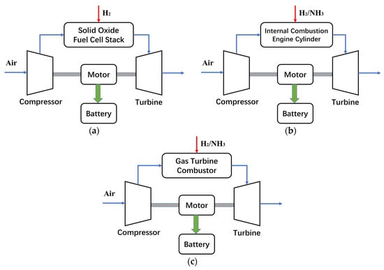
Figure 1.
Schematic of hydrogen turbo hybrid power systems. (a) Hydrogen is oxidized in the SOFC stack. (b) Hydrogen/ammonia is burned in the ICE cylinder. (c) Hydrogen/ammonia is burned in the gas turbine combustor.
To be able to design a turbine to respond to demand quickly, it is important to accurately predict the performance of the radial inflow turbine in both design and off-design conditions. Although computational fluid dynamics (CFD) can replace experiments to obtain turbine performance, turbomachinery designers still tend to use empirical loss models for turbomachinery design and off-design performance analysis, because empirical loss models can provide design results accurately and quickly [5,6,7]. These loss models reflect the irreversibility of turbomachinery and cause a decrease in efficiency as a result [8]. Nevertheless, these loss models are mainly based on subsonic conditions. Modern turbomachine systems are expected to operate in high expansion ratio transonic conditions. Performance prediction is a fundamental part of the preliminary design process of radial inflow turbines and is effectuated using analytical loss models. Analytical loss models are based on theoretical and experimental analyses, which have been developed and refined by many authors. Futral and Wasserbauer proposed the typical formulation of the incidence loss model [9]. Woolley and Hatton conducted flow visualizations for various inlet angles and discovered the optimum relative angle at rotor inlet should be set in the region of −20°~−40° [10]. Wasserbauer and Glassman developed the approach for estimating the rotor passage loss [11], which considers the meridional component of kinetic energy at the inlet and the whole kinetic energy at the exit. Spraker deduced the leakage flow model through the gap between the tip and shroud by modeling the flow through an orifice and a shear flow. Ghosh and Ventura developed the trailing edge loss model based on the total enthalpy loss [12]. A well-known summary of selected loss models was provided by Benson and Baines [6]. The works performed by Benson and Baines are most comprehensive, and the results of these are implanted in many radial inflow turbine design tools.
It is clear from the literature review that the present loss models of the radial turbine are not comprehensive because transonic conditions are not considered. This paper mainly focuses on the comparison of flow field characteristics between subsonic conditions and transonic conditions of a radial inflow turbine. According to the flow field characteristics of the transonic turbine, a shock wave-induced loss model is developed to predict the performance of the transonic turbine more accurately.
2. Numerical Model
A radial inflow vaneless turbine was designed. Table 1 shows the detailed geometry parameters of the turbine.

Table 1.
Detailed geometry of turbine.
The NUMECA software system is used to study the performance and aerodynamics of the turbine in design and off-design conditions, and the structured grid is produced by the NUMECA Autogrid. Figure 2 shows the 3D geometry and meridional cross-section of the turbine. The main geometry parameters are shown in Figure 2b. In order to improve computational efficiency and reduce the number of computational grid cells, a single passage simulation was performed instead of the entire turbine simulation. Figure 3 shows a single passage computing grid.
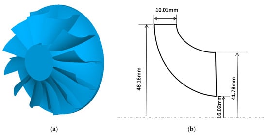
Figure 2.
The 3D geometry and meridional cross-section of turbine. (a) The 3D geometry of turbine. (b) Meridional cross-section of turbine.
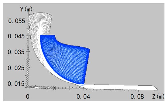
Figure 3.
The computational grids of the single passage.
Before the CFD analysis, a grid study was conducted to check the sensitivity of the grid to the results. The number of the grid has a very important influence on the result of the calculation. If the number is too large, it will waste a lot of time in the calculation. If it is too small, the results of the calculation will be not accurate. So, it is necessary to study the influence of the gridding number on the performance of the turbine. Six types of mesh with different numbers of grid points were generated to calculate the model. The topology of the mesh and the boundary conditions were set the same. Figure 4 shows the effect of gridding numbers on turbine efficiency. It shows that as the number of grids increases, the efficiency of the turbine also increases, but when the number of grids exceeds 700,000, the efficiency remains almost unchanged. Therefore, the final grid number of the rotor grid is close to 700,000, which is higher than the minimum requirement indicated by the grid independence study.
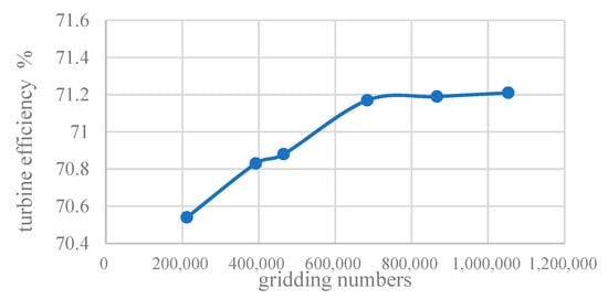
Figure 4.
The grid study.
In order to effectively capture complex 3D flow patterns in the flow channel, HO topology is used in the rotor channel. The mesh topology of the skin blocks around the rotor blades is O topology, and H topology is used in the inlet, outlet and mainstream channel domains. The grid is refined at the near wall, leading edge and trailing edge areas. The rotor blade tip clearance is 0.4 mm. The gap area is gridded by 17 grid points in the span direction. The minimum skew angle of the grid cells is 19. An S-A turbulence model was used as the turbulence model to achieve computational efficiency and good accuracy. For the separated flow, the prediction of the S-A model is better than that of the algebraic model, and the differential equation will not have serious numerical difficulties. Studies have shown that the S-A model is an excellent engineering tool for predicting turbulence characteristics. NUMECA’s solver is FINE/Turbo, which is based on the element-centric finite volume method and is associated with Jameson’s central scheme as spatial discretization and the explicit Runge–Kutta time integration method [13]. The mass flow, velocity direction and temperature are defined at the inlet boundary. The static pressure is defined at the outlet boundary.
In order to verify the accuracy of the simulation results, the experimental results were compared with the simulation results. Figure 5 shows the comparison of the total to static efficiency (the ratio of the actual work output and the theoretical work output based on the rotor pressure drop) between the simulation results and the experimental results. It can be seen from the comparison chart that the model predicts turbine efficiency with high accuracy over a wide expansion ratio (the ratio of the total pressure of the inlet to the static pressure of the outlet) range. In the case of the small expansion ratio, the model prediction value is slightly higher than the experimental value, and the model prediction result is good in the middle section. The predicted value of the model under the large expansion ratio is also slightly higher than the experimental value. However, in general, the simulation calculation results have relatively small errors compared with the test results, and the model has sufficient credibility for the prediction of turbine performance.
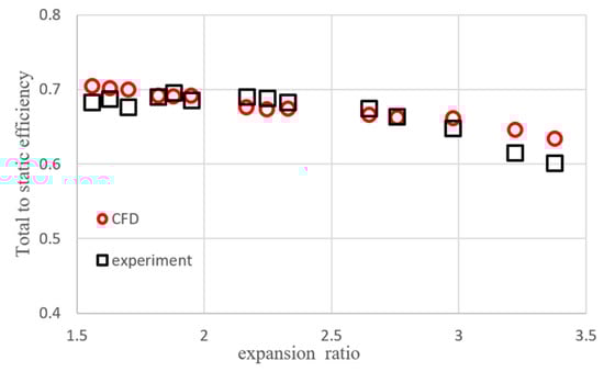
Figure 5.
The total to static efficiency vs. expansion ratio.
3. Flow Fields Characteristics
Figure 6 shows the distribution of the dimensionless velocity divergence at different expansion ratios. The number of the velocity divergence is very large. The dimensionless velocity divergence is the ratio of the velocity divergence to 106. The dimensionless velocity divergence indicates the degree of expansion of the fluid. A positive velocity divergence indicates that the fluid flows from the inside to the outside, and the fluid is expanding; a negative velocity divergence indicates that the fluid flows from the outside to the inside, and the fluid is compressed. For the transonic flow in the turbine rotor passage, the compression processes occur at the shock waves mainly and the leading edge. Therefore, the locations of the shock wave can be determined by regions of negative value in the dimensionless velocity divergence.
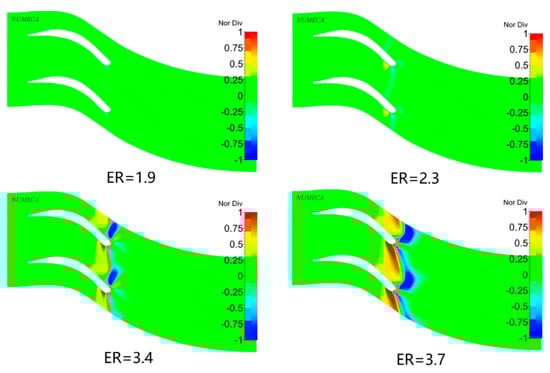
Figure 6.
The distribution of dimensionless velocity divergence at different expansion ratios.
Figure 7 shows the distribution of the relative Mach number at different expansion ratios. Figure 8 shows the distribution of entropy at different expansion ratios. As can be seen from the above figures, with expansion ratio increases, the Mach number at the outlet of the turbine blade becomes larger and larger. At a low expansion ratio, the flow in the turbine is subsonic, and the Mach number at the outlet is less than 1. As the expansion ratio increases, the flow in the turbine changes from subsonic to transonic, and the Mach number at the outlet of the blade is greater than 1.
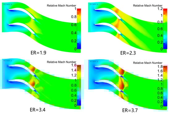
Figure 7.
The distribution of relative Mach number at different expansion ratios.
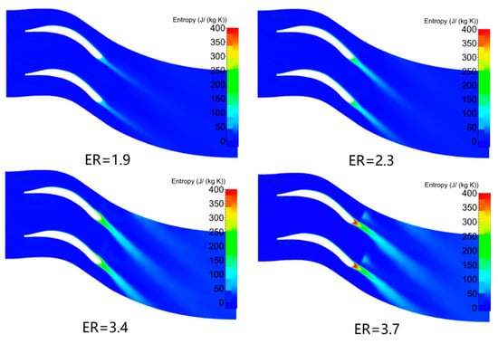
Figure 8.
The distribution of entropy at different expansion ratios.
In the case of a low expansion ratio, the expansion effect of the airflow at the blade outlet is relatively weak, and the Mach number of the airflow in front of the oblique shock wave is relatively low, so the oblique shock wave is relatively weak. With the increase in the expansion ratio, the expansion effect of the airflow at the blade outlet increases, the Mach number in front of the shock wave increases, and the intensity of the corresponding oblique shock wave increases.
Under the condition of a certain expansion ratio, the oblique shock wave on the blade pressure surface occurs at the Mach reflection on the blade suction surface, and an obvious shock wave surface is formed near the outlet of the blade passage. Because of the obvious entropy increase in the flow field caused by the shock wave, flow loss increases, leading to a sharp decrease in turbine efficiency. As the expansion ratio further increases, the Mach number of the oblique shock front further increases, and the oblique shock waves on the blade pressure surface and suction surface intersect at the blade outlet and form a normal shock wave, and there is an obvious entropy increase region behind the shock wave, which induced a great number of losses.
4. Loss Models
The present section on rotor loss models does not attempt to reproduce the full details of the flow in the radial turbine rotor as described in the previous section. There is no way in which the breakdown of the losses occurring in the turbine rotor can be reproduced completely clearly. Any attempt to model losses by dividing them into various categories is logically flawed because all of the losses are interrelated and often interact in some ways. Nevertheless, with some understanding of the physical processes which control the blade passage flow, a reasonable and useful division is possible. As for this paper, the losses are divided into five parts: incidence loss, passage loss, tip clearance loss, trailing edge loss and shock wave-induced loss.
4.1. Incidence Loss
The incidence loss here refers to any work in the turning of the working fluid from its direction of approach to the rotor to the direction required by the blade passage. For an ideal case, the fluid flows into the rotor passage with the optimum incidence angle, which minimizes the entropy generation. However, the fluid may have deviations with the blade angle in most cases. Thus, the incidence loss is the contribution to the entropy generated when the turbine is operating away from its design point, and the rotor inlet flow angle is not equal to the optimum. Although various incidence loss models have been proposed previously, Benson showed similarity of the results for various incidence loss models relative to the variation of the incidence angle. Equation (1) proposed by Futral and Wasserbauer [9] is a typical formulation of this mechanism, where W4 is the relative velocity at the inlet of the rotor, is the incidence angle, and is the optimum incidence angle.
4.2. Passage Loss
Passage loss is a generic term employed for all the losses occurring internally in the blade passage. In a radial turbine rotor, this includes the losses due to cross-stream or secondary flows, the mixing which these bring out, and the blockage and loss of kinetic energy due to the growth of boundary layers and separation. Wasserbauer and Glassman [11] developed the empirical correlation as shown in Equation (2), which considers the meridional component of kinetic energy at the inlet and the whole kinetic energy at the exit, where Kp is a coefficient that should be based on the experimental data and W5 is the relative velocity at the rotor throat.
4.3. Tip Clearance Loss
A clearance gap must be provided between the rotor and its shroud, and consequently, leakage from the rotor blade pressure to suction surfaces occurs. Typically, the clearance gap can be separated into radial clearance and axial clearance. Futral and Holeski showed the effect of tip clearance on the turbine efficiency and the exit flow conditions. It represents that the radial clearance has more impact on the performance of a turbine. Equation (3) proposed by Baines [6] is a typical formulation of this mechanism, where U4 is the velocity of the blade tip, Zr is the number of blades, is the axial clearance, is the radial clearance, , , and
4.4. Trailing Edge Loss
The sudden expansion of the passageway between the throat and exit results in a relative total pressure or kinetic energy loss which is modelled by the trailing edge loss as expressed in Equation (4) [6]. The tangential component of velocity is assumed to be constant, is the radial component of velocity at the rotor throat, and is the radial component of velocity at the outlet.
4.5. Combinations of Four Traditional Losses
The change in total enthalpy at no entropy across the turbine can be calculated as Equation (5), while the total to total efficiency can be calculated as Equation (6). The ratio of loss to is the percentage of losses.is the specific heat ratio of air.
Figure 9 shows the distribution of the four traditional different percentages of losses, which contain the passage loss, the tip clearance loss, the trailing edge loss and the incidence loss. If the loss models can predict the performance of the radial inflow turbine accurately, the sum of the percentage of losses and the total-to-total efficiency will be nearly unity. Figure 9 shows that when the turbine works at a low expansion ratio, the sum of the percentage of losses and the total-to-total efficiency is nearly unity. However, the sum of percentage losses and the total-to-total efficiency is less than unity when the turbine works at high expansion, the largest error is about 10%. This shows that just the traditional four loss models are not suitable for the turbine working at a high expansion ratio. As described in Figure 6, Figure 7 and Figure 8, when the turbine works at a high expansion ratio, its flow is transonic, the shock wave will occur near the outlet and interact with the other flow, and it will cause a number of losses. So, the loss caused by the shock wave cannot be ignored when the turbine works in transonic conditions, and the shock wave-induced model should be developed to make the loss models more complete and accurate.
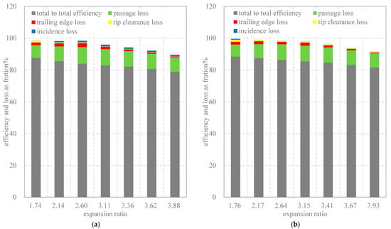
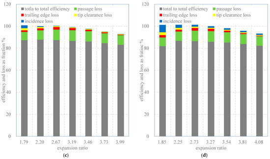
Figure 9.
The distribution of efficiency and the percentage of four traditional losses. (a) 70,000 rpm. (b) 80,000 rpm. (c) 90,000 rpm. (d) 100,000 rpm.
4.6. Shock Wave-Induced Loss
The shock wave-induced loss is caused by the shock wave near the trailing edge in transonic conditions, which contains the loss caused by the shock wave itself and the loss caused by the interaction of shock wave and the boundary layer, the leakage flow and the others. The physical mechanism for this is very uncertain. Equation (7) describes the loss caused by the normal shock wave itself.
Considering the loss caused by the interaction between shock waves and other flows, a loss coefficient needs to be added to the shock wave-induced model as Equation (8).
The loss models and the total to total efficiency should satisfy Equation (9), so the shock wave-induced loss coefficient can be solved.
There are four different rotation speed lines of the turbine as described in Figure 9; the data of rotation speed 70,000 rpm and 100,000 rpm were used to calculate the shock wave-induced loss coefficient and the other data were used to verify whether is correct. SSE means the sum of squares due to error between the left and the right of Equation (9). SSE changes with different shock wave-induced loss coefficients as shown in Figure 10. Figure 10 shows that when is 1.95, the SSE is the smallest. So, the shock wave-induced loss coefficient is determined as 1.95.
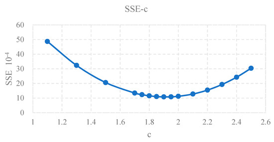
Figure 10.
The SSE vs. c.
The total-to-total efficiency can be predicted by the loss models and Equation (9). Figure 11 shows the error of the predicted efficiency and the CFD efficiency. The solid line represents the error without the shock wave-induced loss model, and the dotted line represents the error with the shock wave-induced loss model. Figure 11 shows that when the expansion ratio is low, the turbine works in subsonic conditions without shock wave loss, so the two kinds of lines are coincident. The two types of lines begin to separate at high expansion ratios, as the shock wave starts to cause losses. The error of the predicted efficiency and the CFD efficiency in high expansion ratio conditions is larger than that in low expansion ratio conditions. The largest error is about 3.5% with the shock wave-induced loss model, much smaller than the 10% without the shock wave-induced loss model. It means that the shock wave-induced loss model can make the prediction of the efficiency more accurate.
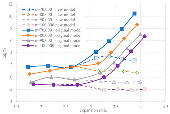
Figure 11.
The error of the predicted efficiency and the CFD efficiency.
Figure 12 shows the distribution of different losses as the fraction of energy when the turbine operates at different expansion ratios and different rotation speeds, which contains the shock wave-induced loss model. The passage loss is the greatest loss of the rotor, which ranges from 8 to 10 percent when the expansion ratio increases and ranges little with the increase of the rotation speed. Tip clearance loss decreases with the increase in the expansion ratio. With the increase in the expansion ratio, the pressure difference between the inlet and the outlet increases, causing the increase in the radial component of velocity at the inlet and at the outlet. So, and will decrease with the increase in the expansion ratio, leading to the decrease in the tip clearance loss. Incidence loss is near zero when the turbine works at the design rotation speed of 80,000 rpm. The farther away from the design speed, the greater the incidence loss. Trailing edge loss increases first then decreases with the increase in the expansion ratio. There is no shock wave-induced loss when the turbine works in subsonic conditions because the shock wave does not occur when the Mach number is below unity. When the expansion ratio is up to 2.6, the turbine starts to work in transonic conditions, and the shock wave occurs, which causes a lot of losses. The turbine starts to work in transonic conditions. As the expansion ratio increases further, the shock wave becomes stronger and stronger, and the shock wave-induced loss increases rapidly.
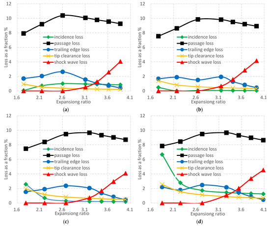
Figure 12.
The distribution of different losses as fraction. (a) 70,000 rpm. (b) 80,000 rpm. (c) 90,000 rpm. (d) 100,000 rpm.
5. Conclusions
In this paper, the flow characteristics and loss models of transonic turbines are studied. With the increase in turbine expansion ratios, an oblique shock wave near the trailing edge will gradually strengthen and move downstream, and finally, the oblique shock wave will turn into a positive shock wave, causing strong shock wave-induced loss. Previous turbine loss models are mainly aimed at subsonic conditions, including incidence loss, passage loss, leakage loss and trailing edge loss without a shock wave-induced loss model of a transonic turbine. In order to predict the performance of transonic turbines more accurately, a shock wave-induced loss model is proposed in this paper. The new combinations of the loss models can make the largest predicted efficiency error decrease from about 10% to 3.5%.
The passage loss is the dominating loss of the turbine, which ranges from 8% to 10%. The tip clearance loss will decrease with the increase in the expansion ratio. The trailing edge loss is about 2% and it will increase first and then decrease as the expansion ratio increases. The closer to the design rotation speed, the lower the incidence loss. The shock wave-induced loss increases rapidly when the turbine works in transonic conditions because of the increase in the Mach number.
Author Contributions
Conceptualization, C.Z., W.Z. and Y.Z.; methodology, C.Z.; formal analysis, C.Z.;investigation, C.Z.; resources, W.Z.; writing—original draft preparation, C.Z.; writing—review and editing, C.Z.; visualization, C.Z.; supervision, Y.Z.; project administration, C.Z.; funding acquisition, W.Z. All authors have read and agreed to the published version of the manuscript.
Funding
This research was supported by the National Key Research and Development Program of China(No. 2020YFB1901702).
Institutional Review Board Statement
Not applicable.
Informed Consent Statement
Not applicable.
Acknowledgments
The authors thank Jie Peng and Yuping Qian for the guidance of the work.
Conflicts of Interest
The authors declare no conflict of interest.
Nomenclature
| ER | expansion ratio (-) |
| L | loss(J/kg) |
| W | velocity in relative frame [m/s] |
| U | velocity of rotor at specific location (radius) [m/s] |
| Ma | Mach number(-) |
| C | velocity in absolute frame [m/s] |
| H | enthalpy [J/kg] |
| K | coefficient for numerous models, refer to model description |
| R | universal Gas Coefficent |
| S | entropy [J/kg-K] |
| T | temperature [K] |
| p | pressure [Pa] |
| Z | number of blades on rotor |
| r | radius [m] |
| t | blade thickness [m] |
| zr | axial length of rotor |
| b | blade height [m] |
| k | ratio of specific heats |
| c | constant number |
| SSE | the sum of squares due to error |
| Greeks | |
| β | flow angle in relative frame |
| ∆ | change in |
| ε | blade clearance [m] |
| η | efficiency (%) |
| Subscripts | |
| tt | total to total |
| 4 | rotor inlet |
| 5 | rotor throat |
| 6 | rotor outlet |
| m | meridional component of velocity |
| i | incidence |
| p | passage |
| clr | tip clearance |
| trl | trailing edge |
| shock | shock wave induced |
| opt | optimal |
| in | rotor inlet |
| out | rotor outlet |
| 0 | stagnation |
| isen | isentropic state |
| ex | exit |
| h | hub of blade |
| t | tip of blade |
| x | axial |
| r | radial |
References
- Rana, K.K.; Natarajan, S.; Jilakara, S. Potential of hydrogen fueled IC engine to achieve the future performance and emission norm. In SAE World Congress & Exhibition; SAE: Detroit, MI, USA, 2015. [Google Scholar]
- Cunanan, C.; Tran, M.K.; Lee, Y.; Kwok, S.; Leung, V.; Fowler, M. A Review of Heavy-Duty Vehicle Powertrain Technologies: Diesel Engine Vehicles, Battery Electric Vehicles, and Hydrogen Fuel Cell Electric Vehicles. Clean Technol. 2021, 3, 474–489. [Google Scholar] [CrossRef]
- Sun, B.; Bao, L.; Luo, Q. Development and trends of direct injection hydrogen internal combustion engine technology. J. Automot. Saf. Energy 2021, 12, 265–278. [Google Scholar]
- Zhou, S.; Yang, W.; Tang, H.; Wang, Y.; Wang, J.; Wang, X.; Yang, F. Research Progress of Ammonia Combustion. China Acad. J. Electron. Publ. House 2021, 41, 4164–4182. [Google Scholar]
- Benson, R.S. A review of methods for assessing loss coefficients in radial gas turbines. Int. J. Mech. Sci. 1970, 12, 905–932. [Google Scholar] [CrossRef]
- Baines, N.C. Part 3: Radial Turbine Design. In Axial and Radial Turbine; Concepts NREC: White River Junction, VT, USA, 2003; pp. 207–239. [Google Scholar]
- Aungier, R.H. Turbine Aerodynamics: Axial-Flow and Radial-Inflow Turbine Design and Analysis; ASME Press: New York, NY, USA, 2006. [Google Scholar]
- Ventura, C.A.M.; Jacobs, P.A. Preliminary Design and Performance Estimation of Radial Inflow Turbines: An Automated Approach. J. Fluids Eng. 2012, 134, 031102. [Google Scholar] [CrossRef]
- Cho, S.K.; Lee, J.I. Comparison of Loss Models for Performance Prediction of Radial Inflow Turbine. Int. J. Fluid Mach. Syst. 2018, 11, 97–109. [Google Scholar] [CrossRef]
- Futral, S.M.; Wasserbauer, C.A. Off-Design Performance Prediction with Experimental Verification for a Radial-Inflow Turbine; Technical Note No.TN D-2621; NASA: Washington, DC, USA, 1965.
- Wasserbauer, C.A.; Glassman, A.J. FORTRAN Program for Predicting the Off Design Performance of Radial Inflow Turbines; Technical Note No.TND-8063; NASA: Washington, DC, USA, 1975.
- Ghosh, S.K.; Sahoo, R.K. Mathematical Analysis for Off-Design Performance of Cryogenic Turboexpander. J. Fluids Eng. 2011, 133, 031001. [Google Scholar] [CrossRef]
- Liu, X.; Wan, K.; Jin, D.; Gui, X. Development of a Throughflow-Based Simulation Tool for Preliminary Compressor Design Considering Blade Geometry in Gas Turbine Engine. Appl. Sci. 2021, 11, 422. [Google Scholar] [CrossRef]
Publisher’s Note: MDPI stays neutral with regard to jurisdictional claims in published maps and institutional affiliations. |
© 2022 by the authors. Licensee MDPI, Basel, Switzerland. This article is an open access article distributed under the terms and conditions of the Creative Commons Attribution (CC BY) license (https://creativecommons.org/licenses/by/4.0/).