
Extension of PAR Models under Local All-Sky Conditions to Different Climatic Zones

 , ,
, , 
Abstract
:1. Introduction
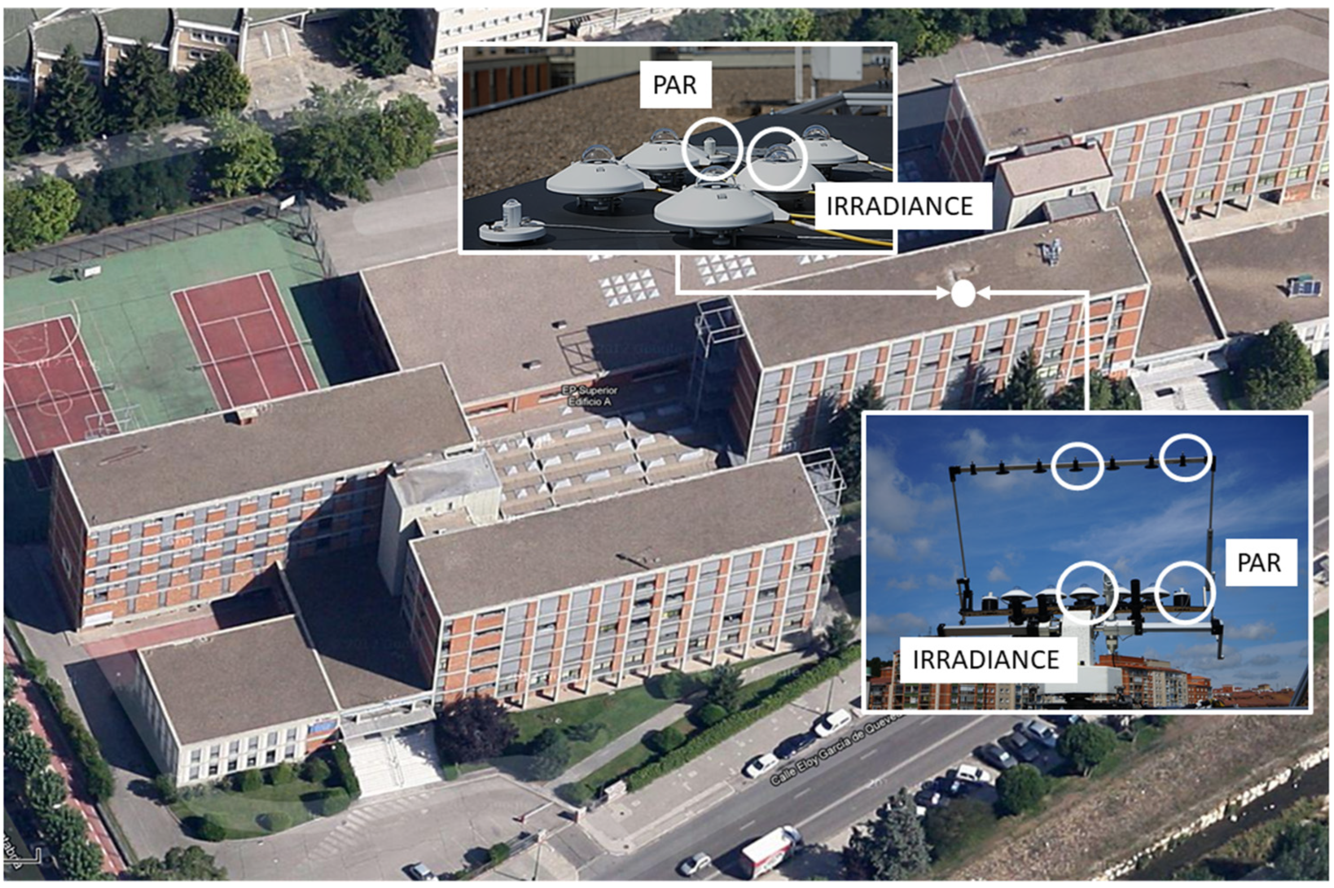
2. Description of the Experimental Data
3. Methodology
3.1. Feature Selection
3.2. Multilinear Regression Models
3.3. Artificial Neural Network Model
4. Extension of the Models to Other Locations
5. Conclusions
Author Contributions
Funding
Data Availability Statement
Acknowledgments
Conflicts of Interest
Abbreviation
| Acronyms | |
| ANN | Artificial Neural Network |
| MPE | Mean Percentage Error |
| MI | Meteorological Index |
| MLR | MultiLinear Regression |
| m.a.s.l. | meters above sea level |
| NOAA | National Oceanic and Atmospheric Administration |
| nRMSE | Normalized Root Mean Square Error |
| nMBE | Normalized Mean Bias Error |
| RSE | Relative Standard Error |
| SURFRAD | Surface Radiation Budget Network |
| Meteorological variables | |
| cosZ | Solar azimuth cosine (°) |
| Δ | Perez’s brightness factor (dim) |
| Perez’s clearness index (dim) | |
| RaGH | Global Horizontal Irradiance (kPa⋅m−2) |
| RaDH | Diffuse Horizontal Irradiance (kPa⋅m−2) |
| RaB | Beam Irradiance (kPa⋅m−2) |
| kd | Horizontal diffuse fraction (dim) |
| kt | Clearness Index (dim) |
| P | Atmospheric Pressure (kPa) |
| PAR | Photosynthetically Active Radiation (kPa⋅m−2) |
| Qp | Photosynthetic photon flux density (μmol⋅s−1⋅m−2) |
| r | Pearson correlation coefficient (dim) |
| RH | Relative Humidity (%) |
| T | Atmospheric Temperature (°C) |
| Td | Dew point temperature (°C) |
References
- Hu, B.; Yu, Y.; Liu, Z.; Wang, Y. Analysis of Photosynthetically Active Radiation and Applied Parameterization Model for Estimating of PAR in the North China Plain. J. Atmos. Chem. 2016, 73, 345–362. [Google Scholar] [CrossRef]
- Qin, W.; Wang, L.; Zhang, M.; Niu, Z.; Luo, M.; Lin, A.; Hu, B. First Effort at Constructing a High-Density Photosynthetically Active Radiation Dataset during 1961–2014 in China. J. Clim. 2019, 32, 2761–2780. [Google Scholar] [CrossRef]
- Sudhakar, K.; Srivastava, T.; Satpathy, G.; Premalatha, M. Modelling and Estimation of Photosynthetically Active Incident Radiation Based on Global Irradiance in Indian Latitudes. Int. J. Energy Environ. Eng. 2013, 4, 21. [Google Scholar] [CrossRef] [Green Version]
- Aguiar, L.J.G.; Fischer, G.R.; Ladle, R.J.; Malhado, A.C.M.; Justino, F.B.; Aguiar, R.G.; da Costa, J.M.N. Modeling the Photosynthetically Active Radiation in South West Amazonia under All Sky Conditions. Theor. Appl. Climatol. 2012, 108, 631–640. [Google Scholar] [CrossRef]
- Landsberg, J.J.; Waring, R.H. A Generalised Model of Forest Productivity Using Simplified Concepts of Radiation-Use Efficiency, Carbon Balance and Partitioning. For. Ecol. Manag. 1997, 95, 209–228. [Google Scholar] [CrossRef]
- Rubio, M.A.; López, G.; Tovar, J.; Pozo, D.; Batlles, F.J. The Use of Satellite Measurements to Estimate Photosynthetically Active Radiation. Phys. Chem. Earth 2005, 30, 159–164. [Google Scholar] [CrossRef]
- Alados, I.; Foyo-Moreno, I.; Alados-Arboledas, L. Photosynthetically Active Radiation: Measurements and Modelling. Agric. For. Meteorol. 1996, 78, 121–131. [Google Scholar] [CrossRef]
- Deo, R.C.; Downs, N.J.; Adamowski, J.F.; Parisi, A.V. Adaptive Neuro-Fuzzy Inference System Integrated with Solar Zenith Angle for Forecasting Sub-Tropical Photosynthetically Active Radiation. Food Energy Secur. 2019, 8, e00151. [Google Scholar] [CrossRef] [Green Version]
- Alados-Arboledas, L.; Olmo, F.J.; Alados, I.; Pérez, M. Parametric Models to Estimate Photosynthetically Active Radiation in Spain. Agric. For. Meteorol. 2000, 101, 187–201. [Google Scholar] [CrossRef]
- López, G.; Rubio, M.; Martinez, M.; Batlles, F. Estimation of Hourly Global Solar Radiation Using Artificial Neural Network. Agric. For. Meteorol. 2001, 107, 279–291. [Google Scholar] [CrossRef]
- Majnooni-heris, A. Estimating Photosynthetically Active Radiation (PAR) Using Air Temperature and Sunshine Durations. J. Biodivers. Environ. Sci. 2014, 5, 371–377. [Google Scholar]
- Vindel, J.M.; Valenzuela, R.X.; Navarro, A.A.; Zarzalejo, L.F.; Paz-Gallardo, A.; Souto, J.A.; Méndez-Gómez, R.; Cartelle, D.; Casares, J.J. Modeling Photosynthetically Active Radiation from Satellite-Derived Estimations over Mainland Spain. Remote Sens. 2018, 10, 849. [Google Scholar] [CrossRef] [Green Version]
- Wang, L.; Gong, W.; Li, C.; Lin, A.; Hu, B.; Ma, Y. Measurement and Estimation of Photosynthetically Active Radiation from 1961 to 2011 in Central China. Appl. Energy 2013, 111, 1010–1017. [Google Scholar] [CrossRef]
- Zempila, M.M.; Taylor, M.; Bais, A.; Kazadzis, S. Modeling the Relationship between Photosynthetically Active Radiation and Global Horizontal Irradiance Using Singular Spectrum Analysis. J. Quant. Spectrosc. Radiat. Transf. 2016, 182, 240–263. [Google Scholar] [CrossRef]
- Ferrera-Cobos, F.; Vindel, J.M.; Valenzuela, R.X.; González, J.A. Models for Estimating Daily Photosynthetically Active Radiation in Oceanic and Mediterranean Climates and Their Improvement by Site Adaptation Techniques. Adv. Space Res. 2020, 65, 1894–1909. [Google Scholar] [CrossRef]
- Mõttus, M.; Ross, J.; Sulev, M. Experimental Study of Ratio of PAR to Direct Integral Solar Radiation under Cloudless Conditions. Agric. For. Meteorol. 2001, 109, 161–170. [Google Scholar] [CrossRef]
- Nwokolo, S.; Amadi, S.O. A Global Review of Empirical Models for Estimating Photosynthetically Active Radiation. Trends Renew. Energy 2018, 4, 236–327. [Google Scholar] [CrossRef] [Green Version]
- Frouin, R.; Pinker, R.T. Estimating Photosynthetically Active Radiation (PAR) at the Earth’s Surface from Satellite Observations. Remote Sens. Environ. 1995, 51, 98–107. [Google Scholar] [CrossRef]
- Vindel, J.M.; Valenzuela, R.X.; Navarro, A.A.; Zarzalejo, L.F. Methodology for Optimizing a Photosynthetically Active Radiation Monitoring Network from Satellite-Derived Estimations: A Case Study over Mainland Spain. Atmos. Res. 2018, 212, 227–239. [Google Scholar] [CrossRef]
- Jacovides, C.P.; Tymvios, F.S.; Boland, J.; Tsitouri, M. Artificial Neural Network Models for Estimating Daily Solar Global UV, PAR and Broadband Radiant Fluxes in an Eastern Mediterranean Site. Atmos. Res. 2015, 152, 138–145. [Google Scholar] [CrossRef]
- Pankaew, P.; Pattarapanitchai, S.; Buntoung, S.; Wattan, R.; Masiri, I.; Sripradit, A.; Janjai, S. Estimating Photosynthetically Active Radiation Using an Artificial Neural Network. In Proceedings of the 2014 International Conference and Utility Exhibition on Green Energy for Sustainable Development (ICUE), Pattaya, Thailand, 19–21 March 2014. [Google Scholar]
- Wang, L.; Kisi, O.; Zounemat-Kermani, M.; Hu, B.; Gong, W. Modeling and Comparison of Hourly Photosynthetically Active Radiation in Different Ecosystems. Renew. Sustain. Energy Rev. 2016, 56, 436–453. [Google Scholar] [CrossRef]
- Yu, X.; Guo, X. Hourly Photosynthetically Active Radiation Estimation in Midwestern United States from Artificial Neural Networks and Conventional Regressions Models. Int. J. Biometeorol. 2016, 60, 1247–1259. [Google Scholar] [CrossRef] [PubMed]
- Peel, M.; Finlayson, B.; McMahon, T. Updated World Map of the Köppen-Geiger Climate Classification. Hydrol. Earth Syst. Sci. 2007, 11, 1633–1644. [Google Scholar] [CrossRef] [Green Version]
- García-Rodríguez, A.; García-Rodríguez, S.; Díez-Mediavilla, M.; Alonso-Tristán, C. Photosynthetic Active Radiation, Solar Irradiance and the Cie Standard Sky Classification. Appl. Sci. 2020, 10, 8007. [Google Scholar] [CrossRef]
- Akitsu, T.; Kume, A.; Hirose, Y.; Ijima, O.; Nasahara, K. On the Stability of Radiometric Ratios of Photosynthetically Active Radiation to Global Solar Radiation in Tsukuba, Japan. Agric. For. Meteorol. 2015, 209–210, 59–68. [Google Scholar] [CrossRef]
- Gueymard, C.A.; Ruiz-Arias, J.A. Extensive Worldwide Validation and Climate Sensitivity Analysis of Direct Irradiance Predictions from 1-Min Global Irradiance. Sol. Energy 2016, 128, 1–30. [Google Scholar] [CrossRef]
- Iqbal, M. An Introduction to Solar Radiation; Academic Press: New York, NY, USA, 1983. [Google Scholar]
- Heating, Refrigerating American Society of y Air Conditing Engineers. American Society of Heating, Refrigerating y Air conditioning Engineers. In ASHRAE Handbook; Ashrae: Atlanta, GA, USA, 2015; ISBN 9781936504459.
- Erbs, D.G.; Klein, S.A.; Duffle, J.A. Estimation of the Diffuse Radiation Fraction for Hourly, Daily and Monthly-Average Global Radiation. Sol. Energy 1982, 28, 293–302. [Google Scholar] [CrossRef]
- Perez, R.; Ineichen, P.; Seals, R.; Michalsky, J.; Stewart, R. Modeling Daylight Availability and Irradiance Components from Direct and Global Irradiance. Sol. Energy 1990, 44, 271–289. [Google Scholar] [CrossRef] [Green Version]
- García-Rodríguez, A.; Granados-López, D.; García-Rodríguez, S.; Díez-Mediavilla, M.; Alonso-Tristán, C. Modelling Photosynthetic Active Radiation (PAR) through Meteorological Indices under All Sky Conditions. Agric. For. Meteorol. 2021, 310, 108627. [Google Scholar] [CrossRef]
- Gueymard, C.A. A Reevaluation of the Solar Constant Based on a 42-Year Total Solar Irradiance Time Series and a Reconciliation of Spaceborne Observations. Sol. Energy 2018, 168, 2–9. [Google Scholar] [CrossRef]
- Suárez-garcía, A.; Granados-lópez, D.; González-peña, D.; Alonso-tristán, C. Benchmarking of Meteorological Indices for Sky Cloudiness Classification. Sol. Energy 2020, 195, 499–513. [Google Scholar] [CrossRef]
- Mukaka, M.M. Statistics Corner: A Guide to Appropriate Use of Correlation Coefficient in Medical Research. Malawi Med. J. 2012, 24, 69–71. [Google Scholar] [PubMed]
- Foyo-Moreno, I.; Alados, I.; Alados-Arboledas, L. A New Conventional Regression Model to Estimate Hourly Photosynthetic Photon Flux Density under All Sky Conditions. Int. J. Climatol. 2017, 37, 1067–1075. [Google Scholar] [CrossRef] [Green Version]
- Du, Y.C.; Stephanus, A. Levenberg-Marquardt Neural Network Algorithm for Degree of Arteriovenous Fistula Stenosis Classification Using a Dual Optical Photoplethysmography Sensor. Sensors 2018, 18, 2322. [Google Scholar] [CrossRef] [PubMed] [Green Version]
- Kottek, M.; Grieser, J.; Beck, C.; Rudolf, B.; Rubel, F. World Map of the Köppen-Geiger Climate Classification Updated. Meteorol. Z. 2006, 15, 259–263. [Google Scholar] [CrossRef]


| MI | MI | Expression | Ref. |
|---|---|---|---|
| RaGH | Global Horizontal Irradiance | recorded | |
| kd | Horizontal diffuse fraction | [30] | |
| Qp | Photosynthetic photon flux density | recorded | |
| PAR | Photosynthetically active radiation | [26] | |
| kt | Clearness index | [28] | |
| T | Air temperature | recorded | |
| P | Pressure | recorded | |
| Td | Dew point temperature | [29] | |
| cosZ | Solar azimuth cosine | [28] | |
| ε | Perez’s clearness index | [31] | |
| Δ | Perez’s Brightness factor | [31] |
| |r (PAR, MIi)| | |||||
|---|---|---|---|---|---|
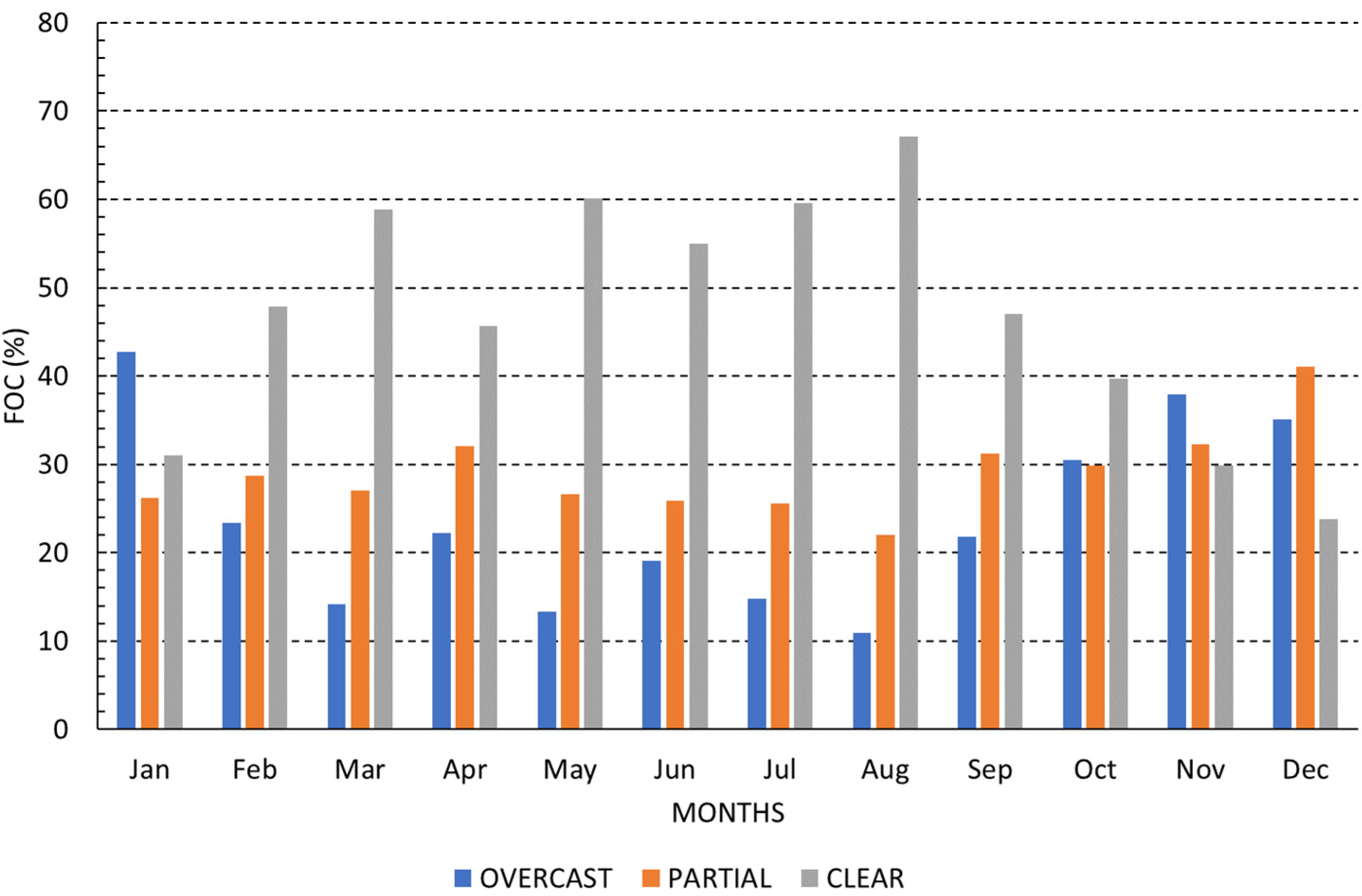
| kt Sky Type | [1–0.9] | (0.9–0.7] | (0.7–0.5] | (0.5–0.3] | (0.3,0] |
| All sky conditions | RaGH | cosZ, kt | kd, ε | T | Δ, P, Td |
| Clear | RaGH, cosZ | kt, ε | T | kd, Δ, P, Td | |
| Partial | RaGH, cosZ | T | kt, kd, Δ, ε, P, Td | ||
| Overcast | RaGH | cosZ | kt, Δ | kd, ε, P, T, Td | |
| Sky Conditions | Multilinear Regression Model | nRMSE (%) | nMBE (%) | |
|---|---|---|---|---|
| All skies (MLR1) | 0.994 | 4.37 | −2.74 × 10⁻¹³ | |
| Clear skies (MLR2) | 0.990 | 3.27 | −1.45 × 10⁻¹⁴ | |
| Partial skies (MLR3) | 0.977 | 6.80 | −5.32 × 10⁻¹³ | |
| Overcast skies (MLR4) | 0.978 | 7.33 | 1.87 × 10⁻¹³ |
| Sky Conditions | nRMSE (%) | nMBE (%) | |
|---|---|---|---|
| All skies (ANN1) | 0.994 | 4.22 | 2.84 × 10⁻³ |
| Clear skies (ANN2) | 0.992 | 3.01 | −4.68 × 10⁻² |
| Partial skies (ANN3) | 0.977 | 6.80 | 4.06 × 10⁻³ |
| Overcast skies (ANN4) | 0.978 | 7.28 | −3.50 × 10⁻² |
| Sky Conditions | nRMSE (%) | nMBE (%) | Sky Conditions | nRMSE (%) | nMBE (%) | ||
|---|---|---|---|---|---|---|---|
| All skies (MLR1) | 0.994 | 4.48 | −5.20 × 10⁻³ | All skies (ANN1) | 0.994 | 4.35 | −4.00 × 10⁻³ |
| Clear skies (MLR2) | 0.992 | 3.00 | 1.21 × 10⁻¹ | Clear skies (ANN2) | 0.993 | 2.782 | 4.89 × 10⁻² |
| Partial skies (MLR3) | 0.978 | 6.72 | −6.02 × 10⁻² | Partial skies (ANN3) | 0.978 | 6.71 | −5.26 × 10⁻² |
| Overcast skies (MLR4) | 0.982 | 6.63 | −4.84 × 10⁻² | Overcast skies (ANN4) | 0.982 | 6.59 | −5.10 × 10⁻¹ |
| Latitude (°N) | Latitude (°W) | Altitude (m.a.s.l.) | Climate | |
|---|---|---|---|---|
| Bondville, Illinois | 40.05192 | 88.37309 | 230 | Dfa |
| Table Mountain, Boulder, Colorado | 40.12498 | 105.2368 | 1689 | Bsk |
| Desert Rock, Nevada | 36.62373 | 116.01947 | 1007 | Bwh |
| Fort Peck, Montana | 48.30783 | 105.1017 | 634 | Bsk |
| Goodwin Creek, Mississippi | 34.2547 | 89.8729 | 6 | Cfa |
| Penn State, Univ. Pennsylvania | 40.72012 | 77.93085 | 376 | Dfb |
| Sioux Falls, South Dakota | 43.73403 | 96.62328 | 473 | Dfa |
| MLR | ANN | |||||
|---|---|---|---|---|---|---|
| USA Stations | nRMSE (%) | nMBE (%) | nRMSE (%) | nMBE (%) | ||
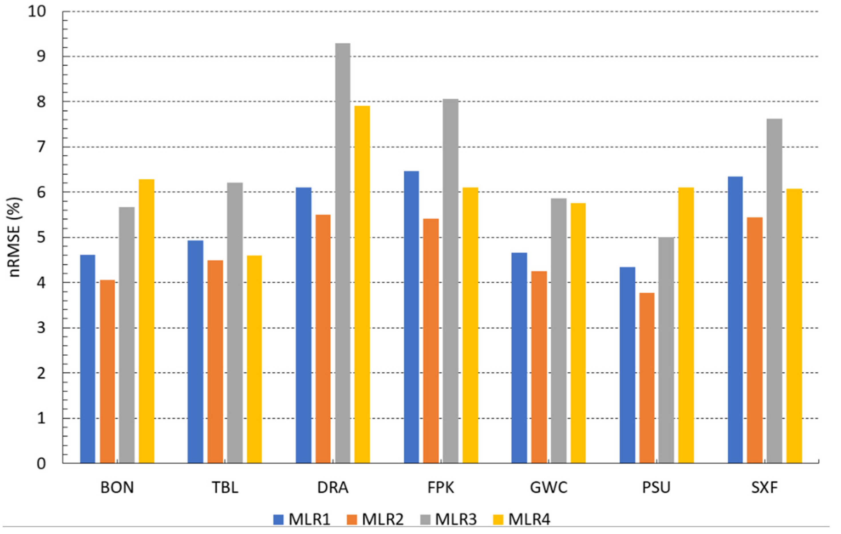
| Bondville, Illinois | 0.994 | 4.62 | 1.89 | 0.994 | 4.90 | 2.54 |
| Table Mountain, Boulder, Colorado | 0.996 | 4.93 | 3.48 | 0.996 | 5.48 | 4.18 |
| Desert Rock, Nevada | 0.997 | 6.10 | 5.36 | 0.997 | 6.75 | 6.04 |
| Fort Peck, Montana | 0.994 | 6.46 | 4.94 | 0.994 | 6.87 | 5.45 |
| Goodwin Creek, Mississippi | 0.995 | 4.66 | 2.48 | 0.995 | 5.15 | 3.33 |
| Penn State, Univ. Pennsylvania | 0.995 | 4.35 | 1.34 | 0.995 | 4.62 | 2.07 |
| Sioux Falls, South Dakota | 0.995 | 6.34 | 5.00 | 0.995 | 6.84 | 5.59 |
| MLR | ANN | |||||
|---|---|---|---|---|---|---|
| USA Stations | nRMSE (%) | nMBE (%) | nRMSE (%) | nMBE (%) | ||
| Bondville, Illinois | 0.985 | 4.05 | 1.61 | 0.985 | 4.13 | 1.28 |
| Table Mountain, Boulder, Colorado | 0.993 | 4.50 | 3.30 | 0.992 | 4.67 | 3.13 |
| Desert Rock, Nevada | 0.994 | 5.50 | 4.87 | 0.994 | 5.77 | 4.77 |
| Fort Peck, Montana | 0.988 | 5.41 | 4.16 | 0.987 | 5.31 | 3.74 |
| Goodwin Creek, Mississippi | 0.985 | 4.25 | 2.37 | 0.984 | 4.46 | 2.06 |
| Penn State, Univ. Pennsylvania | 0.987 | 3.77 | 1.20 | 0.986 | 4.02 | 0.95 |
| Sioux Falls, South Dakota | 0.991 | 5.44 | 4.49 | 0.990 | 5.36 | 4.03 |
| MLR | ANN | |||||
|---|---|---|---|---|---|---|
| USA Stations | nRMSE (%) | nMBE (%) | nRMSE (%) | nMBE (%) | ||
| Bondville, Illinois | 0.990 | 5.66 | 3.15 | 0.990 | 5.67 | 3.19 |
| Table Mountain, Boulder, Colorado | 0.994 | 6.21 | 4.67 | 0.994 | 6.24 | 4.72 |
| Desert Rock, Nevada | 0.996 | 9.29 | 8.23 | 0.996 | 9.33 | 8.31 |
| Fort Peck, Montana | 0.991 | 8.06 | 6.51 | 0.991 | 8.08 | 6.56 |
| Goodwin Creek, Mississippi | 0.992 | 5.87 | 4.00 | 0.992 | 5.90 | 4.04 |
| Penn State, Univ. Pennsylvania | 0.991 | 5.00 | 2.27 | 0.991 | 5.00 | 2.30 |
| Sioux Falls, South Dakota | 0.992 | 7.62 | 6.22 | 0.992 | 7.64 | 6.26 |
| MLR | ANN | |||||
|---|---|---|---|---|---|---|
| USA Stations | nRMSE (%) | nMBE (%) | nRMSE (%) | nMBE (%) | ||
| Bondville, Illinois | 0.984 | 6.29 | −0.23 | 0.984 | 7.13 | 3.32 |
| Table Mountain, Boulder, Colorado | 0.992 | 4.60 | 0.70 | 0.992 | 6.23 | 4.18 |
| Desert Rock, Nevada | 0.993 | 7.91 | 5.81 | 0.993 | 11.07 | 9.40 |
| Fort Peck, Montana | 0.989 | 6.11 | 2.61 | 0.988 | 8.48 | 6.37 |
| Goodwin Creek, Mississippi | 0.987 | 5.75 | 0.19 | 0.986 | 6.82 | 3.48 |
| Penn State, Univ. Pennsylvania | 0.987 | 6.11 | −1.67 | 0.987 | 6.15 | 1.91 |
| Sioux Falls, South Dakota | 0.989 | 6.07 | 1.88 | 0.988 | 8.14 | 5.54 |
Publisher’s Note: MDPI stays neutral with regard to jurisdictional claims in published maps and institutional affiliations. |
© 2022 by the authors. Licensee MDPI, Basel, Switzerland. This article is an open access article distributed under the terms and conditions of the Creative Commons Attribution (CC BY) license (https://creativecommons.org/licenses/by/4.0/).
Share and Cite
García-Rodríguez, A.; García-Rodríguez, S.; Granados-López, D.; Díez-Mediavilla, M.; Alonso-Tristán, C. Extension of PAR Models under Local All-Sky Conditions to Different Climatic Zones. Appl. Sci. 2022, 12, 2372. https://doi.org/10.3390/app12052372
García-Rodríguez A, García-Rodríguez S, Granados-López D, Díez-Mediavilla M, Alonso-Tristán C. Extension of PAR Models under Local All-Sky Conditions to Different Climatic Zones. Applied Sciences. 2022; 12(5):2372. https://doi.org/10.3390/app12052372
Chicago/Turabian StyleGarcía-Rodríguez, Ana, Sol García-Rodríguez, Diego Granados-López, Montserrat Díez-Mediavilla, and Cristina Alonso-Tristán. 2022. "Extension of PAR Models under Local All-Sky Conditions to Different Climatic Zones" Applied Sciences 12, no. 5: 2372. https://doi.org/10.3390/app12052372
APA StyleGarcía-Rodríguez, A., García-Rodríguez, S., Granados-López, D., Díez-Mediavilla, M., & Alonso-Tristán, C. (2022). Extension of PAR Models under Local All-Sky Conditions to Different Climatic Zones. Applied Sciences, 12(5), 2372. https://doi.org/10.3390/app12052372