Modelling Automated Planning Problems for Teams of Mobile Manipulators in a Generic Industrial Scenario

Abstract

Flexible control strategies are required in industrial scenarios to coordinate the actions of mobile manipulators (e.g., robots and humans). Temporal planning approaches can be used as such control strategies because they can generate those actions for the agents that must be executed to reach the goals, from any given state of the world. To deploy such approaches, planning models must be formulated. Although available in the literature, these models are not generic enough such that they can be easily transferred to new use cases. In this work, a generic industrial scenario is derived from real scenarios. For this scenario, a generic planning problem is developed. To demonstrate their generality, the two constructs are configured for a new scenario, where custom grippers are assembled. Lastly, a validation methodology is developed for the generic planning problem. The results show that the generic industrial scenario and the generic planning problem can be easily instantiated for new use cases, without any new modelling. Further, the proposed validation methodology guarantees that these planning problems are complete enough to be used in industrial use cases. The generic scenario, the planning problems, and the validation methodology are proposed as standards for use when deploying temporal planning in industrial scenarios with mobile manipulators.

1. Introduction

With the increasing complexity of industrial use cases, it becomes necessary that agents (humans and robots) cooperate in teams to reach more elaborate goals. The complexity of these goals is given by the actions that must be carried out by the agents in order to achieve them. Repetitive actions that must be executed in a fixed order and by specific agents are replaced by flexible processes where more agents cooperate in a shared environment. The complexity of such scenarios is further increased if the teams of agents are heterogeneous, consisting of humans and robots. To coordinate the actions of these agents, considering their capabilities, the status of the world, and the complexity of the goals, automated task planning approaches (also known as AI planning) can be used as high-level control strategies. These approaches offer the planning flexibility required by real-world use cases in which changing initial and goal states are expected. With these approaches, a high autonomy of the involved robots can be achieved.

In order to deploy AI task planning approaches in such industrial use cases, task planning models must be formulated and validated. In the related literature, a couple of such models have already been presented [1,2,3,4]. However, for each industrial use case, an individualized planning model is formulated. This individualized solution complicates the transfer of planning models among diverse industrial use cases and the development of a generic validation methodology. Such a methodology is used to guarantee that the task planning models cover a large number (if not all) possible planning situations. A new planning situation for an industrial scenario can occur when new orders (e.g., goals) are received, and the high-level control module must generate a series of actions from a new state of the world to a state in which the new goals are reached.

To overcome the shortcoming presented above, in this work, a generic industrial scenario description is determined based on a set of industrial scenarios surveyed from the literature. For this generic industrial scenario, a generic planning problem is developed. To demonstrate the generality of this model, it is configured for a new industrial scenario in which customized grippers are assembled. All planning models are formulated as temporal planning problems in the Planning Domain Definition Language (PDDL). Lastly, a generic validation method is presented that checks a set of criteria (e.g., solvability, makespan) for many possible variations of the planning problems for a configuration of the generic planning problem, for a specific industrial scenario.

2. Related Work

Task planning is already used in several competitions and research projects to generate and orchestrate the actions of the involved actors. In this section, a set of scenarios is selected where the scenarios have characteristics specific to those of industrial use cases. These scenarios are analysed with respect to the number and types of the considered actors, the actions to be executed, and the environments in which the entire setup is built. Further on, the question of which types of planning strategies and planning models are used is considered. This is mainly differentiated between more flexible planning approaches such as automated planning [5], and more rigid approaches such as finite state machines (FSMs) or behaviour trees (BTs) [6].

2.1. Competitions

The RoboCup is an international initiative for promoting research in robotics and artificial intelligence. In 2020, more than five leagues were organized, including RoboCup@Work and the RoboCup Logistics League [7].

2.1.1. RoboCup@Work

The RoboCup@Work competition is oriented towards industrial scenarios with mobile manipulators and covers a large spectrum of current research topics related to the factory of the future. One of the main focuses is set on the automation of the reasoning, planning, and scheduling processes [8,9].

The document that sets the guidelines for the competition is its Rulebook [10]. The 2020 version contains the description of the competing robots and of the environment, as well as the scenarios with their required actions. Each competing robot must be able to navigate and has a manipulator with an end-effector that enhances it with the capability of grasping a limited number of objects from the environment. The most important actions that must be executed by the robots are “loading and/or unloading of containers with/of objects with the same or different size; pickup or delivery of parts from/to structured storages and/or unstructured heaps; operation of machines, including pressing buttons, opening/closing doors and drawers, and similar operations with underspecified or unknown kinematics; […] cooperative assembly of non-trivial objects, with other robots and/or humans; […] cooperative transportation of objects (robots with robots, robots with humans)”. The environment consists of a building-like structure with walls delimiting rooms and corridors. In the environment, places are defined as locations, usually correlated to service areas where, for example, a specific task must be executed. On the service areas different objects can be found [9].

Complex task planning capabilities are required to organize the actions of the competing robots only for a small part of the competition’s tests. In most of the tests, the order of the actions is imposed by the quite strict order in which the sub-goals must be achieved. Thus, the required actions are usually organized through small optimization approaches or FSMs [11,12]. In the Basic Transportation Test, in which a set of objects must be moved from one service area to another and which involves both navigation and manipulation activities [9], more complex task planning strategies are required. For example, the b-it-bots team used the automated planner Mercury [13] in the 2017 competition, with simpler FSMs in a three-layer architecture [14]. In the 2019 competition, instead of an automated planner, the robOTTO team used an optimizer integrated into a similar architecture [15].

2.1.2. RoboCup Logistics League

The RoboCup Logistics League (RCLL) focuses on a logistic scenario in a smart factory environment. The environment is partially surrounded by walls, inside which seven machines for each team are randomly distributed. The available machines are of four types, and each is responsible for a specific processing step. The competing robots (three for each team) have the task of transferring objects between processing stations to assemble a final product. The robots have a Robotino mobile base [16] on which an extension tower with a platform is mounted. The tower has a specific height that allows an attached gripper to reach the conveyor belt inputs and outputs of all machines [7,17].

From the task planning point of view, the most demanding part of the competition is the production phase. The robots can execute mainly three types of physical actions: navigating, loading, and unloading, but the challenge is to determine their optimal sequence to carry out the given orders. For this purpose, different scheduling and task planning approaches are deployed. The more complex approaches are integrated in a multi-layer planning–execution architecture, while the more rigid approaches are directly connected to the lower-level hardware. For example, the GRIPS team [18] used a hierarchical task network (HTN) approach for the 2020 competition, in which the main goals are decomposed to basic actions. Then, a scheduler sends the generated sub-tasks according to some priority rules to the idle robots. The Carologistics team [19] used automated planners in the 2018 competition, integrated into the CLIPS executor [20] to plan the actions required to reach the sub-goals determined in a previous step from the received orders. Other participants, such as the robOTTO team [21], have used an optimizer to generate sub-tasks that are implemented on the lower level with FSMs. The entire planning and execution process was also implemented only through FSMs, for example, by the ER-Force team [22] and the Solidus team [23] in the 2018 competition.

An interesting point of view is presented in [24], where it is argued that the most successful teams in RCLL competitions in the last few years, Carologistics [19] and GRIPS [18], used quite simple approaches that focused more on task scheduling, than on task planning. The authors also suggest a series of measures to foster the planning aspects. One such measure could be to remove the hard requirements to process a specific piece only at a specific location. Another option could be to allow the robots of the team to carry more items at a time or just to scale up the problem by adding more robots, more objects, or more stations.

Another competition that uses a domain similar to the one used in RCLL competitions is the Planning and Execution Competition for Logistics Robots in Simulation [25]. In the 2018 edition, only three teams participated, all of them using automated planners for organizing the actions for the competing robots [26]. Two teams used ASP-based planners [27], while the third used the temporal planner POPF [28], with the ROSPlan framework [29].

2.2. Research Projects

Apart from the competitions, many other research projects integrate task planning and scheduling approaches in industrial scenarios. At the competitions, different teams try to solve the same, more generic problems, but in each research project, only one team is usually tackling a more specific challenge. Thus, new insights related to task planning and scheduling can be gathered.

In [30], multi-agent planning is combined with automated task planning. The latter is used by each agent to determine the optimal order of the actions to be executed such that the goals originating from the highest-level planning module are reached. The setup of the scenarios considered in this work is in an industrial environment, where a mobile manipulator has the following skills: navigating, picking, and placing objects from and on pallets.

An industrial collaborative scenario in which a human is supported by a cobot, a KUKA LBR iiwa, in executing a set of manipulation tasks is used in [31]. The actions of the two actors are planned dynamically using HTNs. A similar industrial process, an assembly process, in which a human and one or more serial manipulators are involved, is considered in [32]. All actors have a set of assembly and manipulation skills and are able to communicate between themselves. To coordinate their actions, the upper-level task planning creates sequences of skills for each of the actors. These skills are then implemented as complex FSMs and directly control the hardware of the robot or give clear commands to the human.

3. Materials and Methods

Based on the related work, a generic industrial scenario (GIS) with mobile manipulators is firstly introduced. Afterwards, a generic planning problem (GPP) developed for the GIS and a suitable validation method for it and its instances are presented.

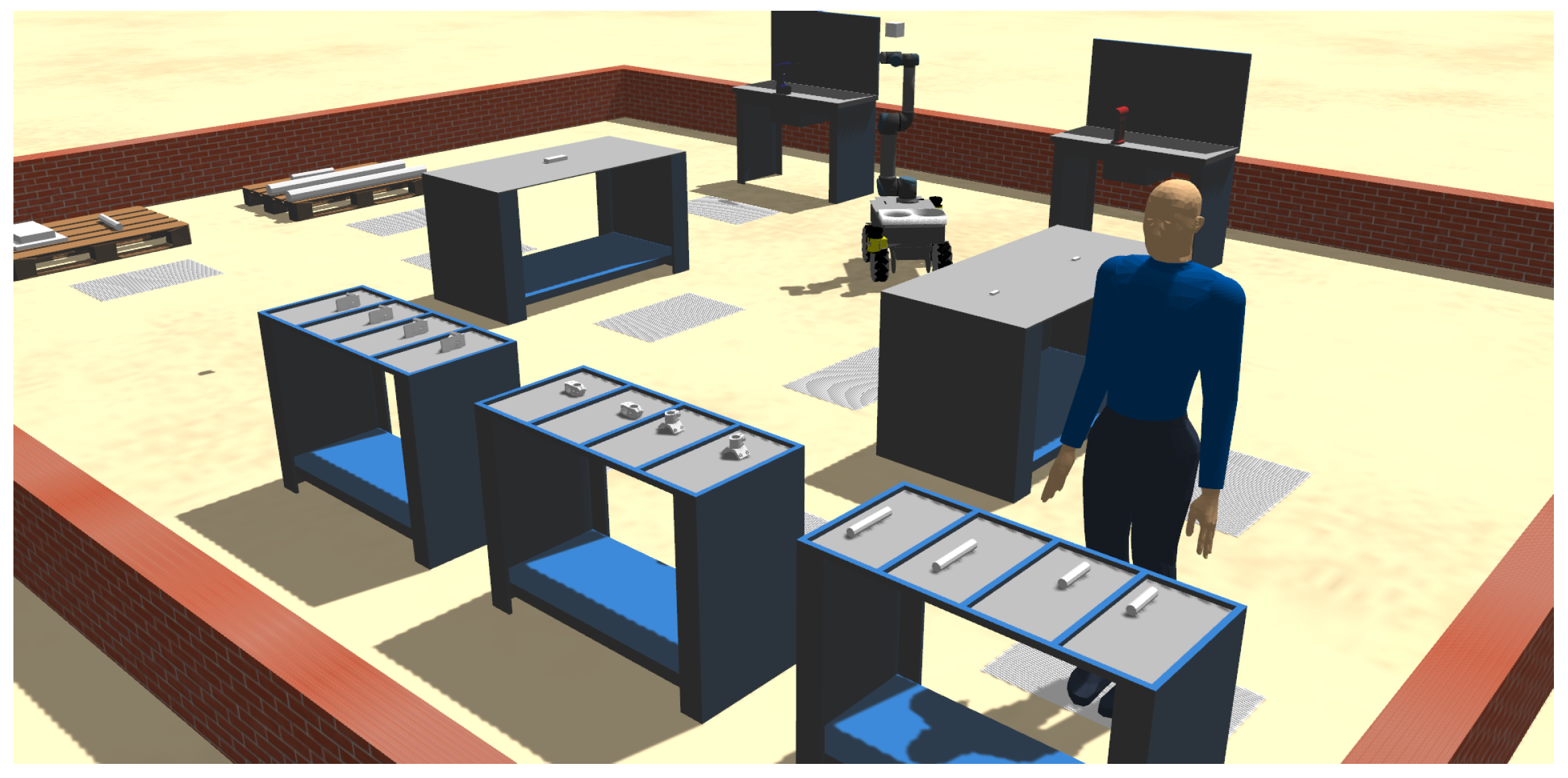
3.1. Modelling a Generic Industrial Scenario (GIS)

A generic industrial scenario (GIS) was derived from the scenarios reviewed in Section 2. The GIS aimed to bring together all characteristics related to the actors, environment, and processes that are similar among these scenarios. The GIS should become a standard model that can be instantiated to any further industrial scenario with mobile manipulators. An instance of the generic scenario (IGIS) is just a specification of all its properties with respect to those of a specific scenario, with specific actors and processes and within a specific environment. The instantiation process does not require any new modelling.

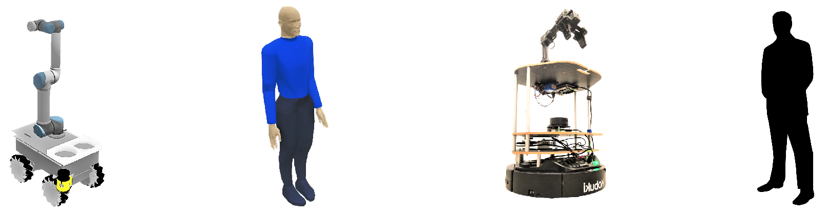
3.1.1. Actors Modelling

In the scenarios reviewed in Section 2, robots or mixed teams of robots and humans are involved. Both types of actors share a set of specific capabilities. This motivates their abstraction as part of the GIS to a generic actor type: a mobile manipulator. A mobile manipulator is an agent that is able to navigate in the environment, and thus has a mobile base and is able to execute trajectories with a serial arm. The agent can also grasp and release items and tools from the environment with the end of that arm.

We differentiate between simulated mobile manipulators and real mobile manipulators (see Figure 1). Given their capabilities, the mobile manipulators can execute a set of specific actions and types of actions. The actions considered in this work are:

• navigate: This action allows an actor to navigate between two poses;
• grasp/place: This action allows an actor to grasp/place an item or a tool from/to a known location from the environment, from itself, or from another actor;
• fetch/discard: This action allows an actor to fetch/discard an item or a tool from the environment with an unknown location;
• connect: This action allows an actor to connect two items from the environment;
• manipulate: This type of action allows an actor to manipulate and process items from the environment. Possible manipulation actions are: screw, press_button, etc.;
• collaboration: This type of action allows two actors to collaborate when executing one action.

The advantage of abstracting the capabilities of the two kinds of actors to those of a mobile manipulator is further leveraged in the development of the GPP for the GIS.

3.1.2. Environment Modelling

The generic environment of the GIS is an indoor environment that is composed of one or more rooms connected by a corridor, into which the agents can travel through doors. As well as the wall structures, different types of benches are also present in the environment. They are: itemsbenches, toolbenches, and workbenches. As the names suggest, items related to the scenario are stored at itemsbenches and tools can be found at toolbenches. The manipulation and the processing of the items is intended to take place at the workbenches. Each bench has a set of poses which the agents can travel to, the agentposes, and can have a set of poses where items can be stored, the itemposes, and a set of poses where tools can be stored, the toolposes.

While the environment is only the static part of the GIS, moving and changing items and tools must also be integrated. Items can be manipulated, moved, and modified, but cannot make changes in the environment by themselves. Tools can be manipulated and moved. In addition, tools can modify items. For example, a tool can be designed as a hand drill that is able to modify a gear, which is in this case a specialization of an item.

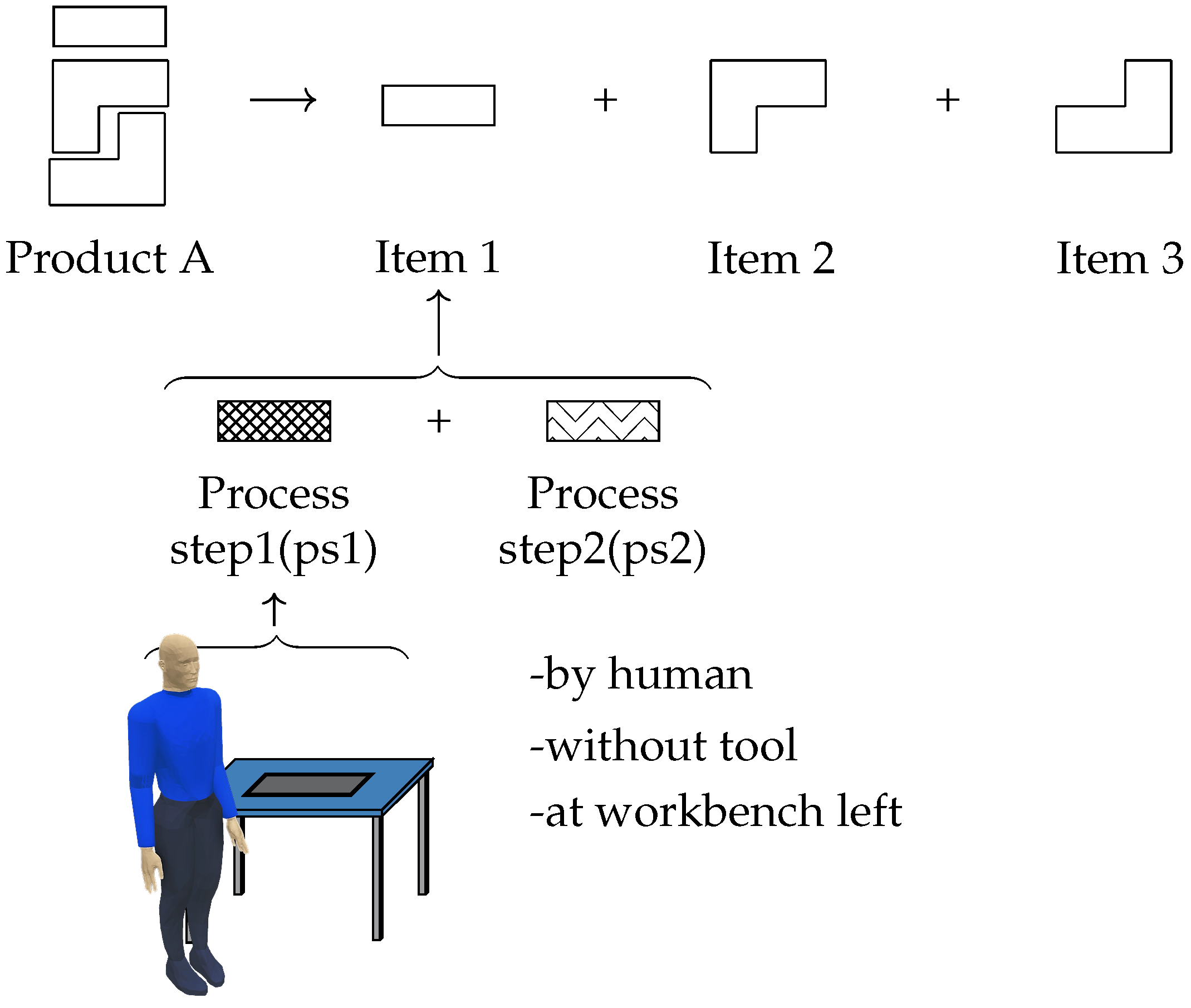
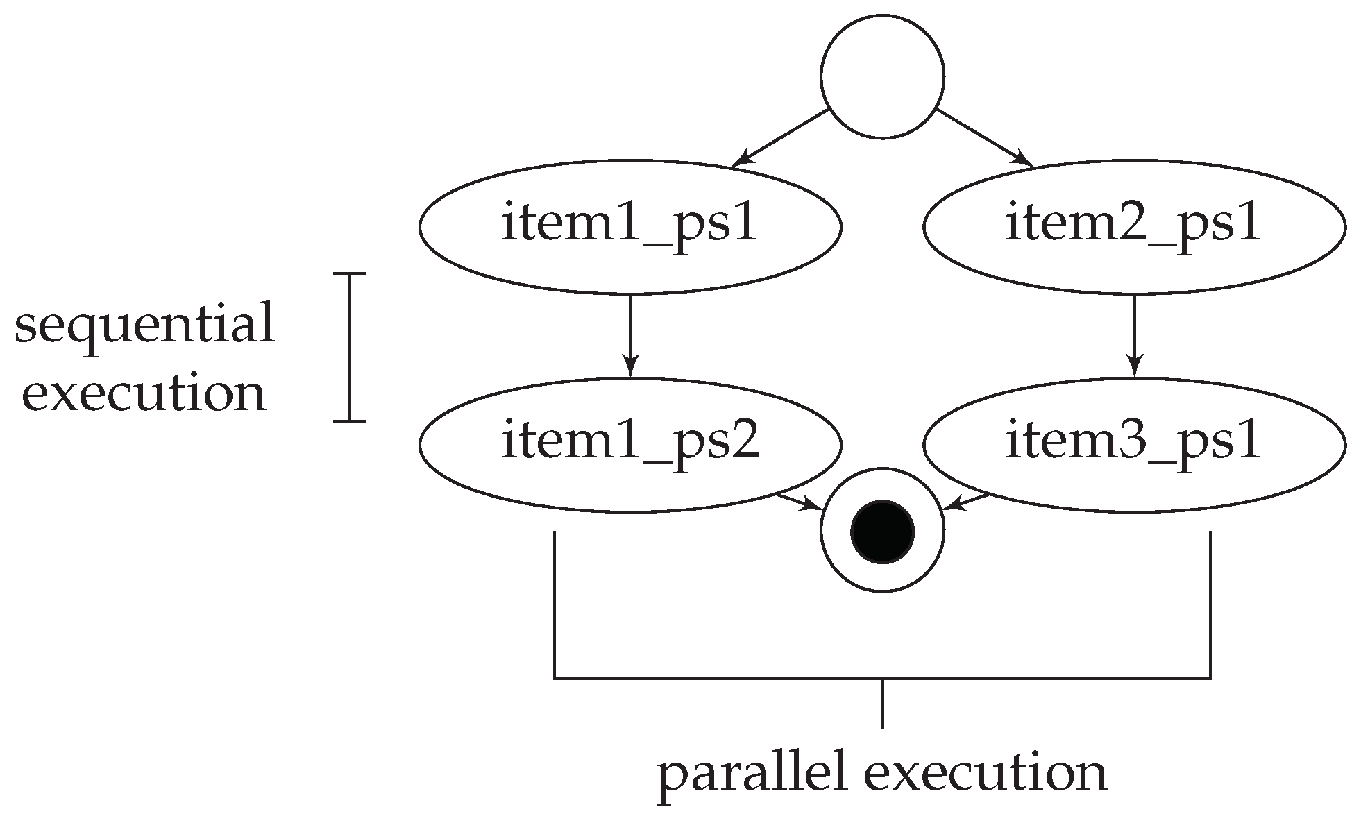
3.1.3. Processes Modelling

A generic process of the GIS is composed of different process steps that are assigned to specific items. Each process step describes how the item must be modified, at which location, with which tool, and by which agent. Furthermore, time dependencies between different process steps exist. These dependencies are also part of the generic process representation.

The generic process representation is explained for the following example in which a product A must be assembles from three items. One or more process steps must be carried out on each of the three items. We assume that two process steps must be executed on the first item, and on the other two items only one process step must be executed. The first process step of item1 must be carried out by a human, without a tool, and at the left workbench. Figure 2 presents an abstract description of these process steps.

The process steps of the three items can be performed sequentially or in parallel, depending on the description of the complete assembly process. The dependencies between the process steps of one item or of different items can be described with activation rules. Once a process step of an item has successfully finished, one or more process steps of one or more items can be activated. Figure 3 depicts the activation rules for the four process steps of the example presented above. The two process steps on item1 must be executed sequentially. During the execution of the two process steps on item1, the process step1 on item2 and the process step1 on item3 can also be carried out. In the final state, the product A is complete.

3.2. The Generic Planning Problem (GPP) for the GIS and Its Instances in PDDL

To increase the automation degree of industrial processes with robotic mobile manipulators, automated planning methods can be used as a high-level control strategy. As presented in the related work in Section 2, automated planning approaches offer high execution flexibility and autonomy to the system and are already deployed in a large number of real-world applications. Different automated planning approaches exist. Planning problems can be formulated as classical or temporal planning problems [5] in the Planning Domain Definition Language (PDDL) [33], as hierarchical task networks (HTN) [34], or as flexible timelines [35] and solved with corresponding solver. Each planning approach has its advantages and disadvantages. However, their comparison is not the topic of this work and is not discussed further here.

In this work, we focus on the formulation of a generic planning problem (GPP) for the generic industrial scenario (GIS). Furthermore, we describe how instances of the generic planning problem (IGPPs) can be derived for IGISs. Both the GPP and the IGPPs are formulated as temporal planning problems in PDDL. The following lines briefly introduce the theoretical aspects of classical and temporal planning problems, as well as the Planning Domain Definition Language that was used for the formulation of these planning problems.

Definition 1.

A classical planning problem Π is a 4-tuple $\mathrm{\Pi }=\langle S,A,s_0,g\rangle$ where S is a finite set of states s described with state variables x, A is a finite set of actions where every action $a\in A$ has some preconditions $a_{\mathit{pre}}$ and effects $a_{\mathit{eff}}=\langle a_{\mathit{add}},a_{\mathit{del}}\rangle$, $s_0\in S$ is the initial state, and g is a set of goals. A solution to the planning problem is a plan π containing a set of grounded actions $a_i\in A$ that bring the system from $s_0$ to a goal state in which the goals from g hold.

In PDDL, classical planning problems are described in two different files. The domain file contains the definition of object types, predicates, and actions. PDDL object types are classes (e.g., item) for which instances are defined in the problem file (e.g., corner, tube); PDDL predicates p correspond to the state variables x from Definition 1 and have as parameters one or more objects types; PDDL actions correspond to the action $a\in A$ from Definition 1 and have as parameters zero or more object types.

Definition 2.

A predicate p or an action a is called grounded if all its parameters are instantiated to objects (e.g., corner) of the corresponding object type (e.g., item).

In this context, a state $s\in S$ from Definition 1 is described by a list of true grounded predicates. Grounded predicates that do not hold (e.g., are false) are not part of the description. The initial state $s_0$ and the goals g of the planning problem $\mathrm{\Pi }$ are also formulated as a list of grounded predicates. The initial state and the goals, together with the instantiated object types, form the second PDDL file, i.e., the problem file.

A solution to a planning problem $\mathrm{\Pi }=\langle S,A,s_0,g\rangle$ is the plan $\pi =[a_1,\dots ,a_n]$, containing grounded actions $a_i$. The actions $a_i$ are selected and grounded in the solving process such that their preconditions $a_{\mathit{pre}}$ hold in the state $\widetilde{s_i}$ to which they are applied (e.g., $a_1$ is applied to $s_0$). Furthermore, each $a_i$ applies to the state $\widetilde{s_i}$ add and del effects. The add effects extend the description of $\widetilde{s_i}$ with new grounded predicates, while the del effects remove grounded predicates from the description of $\widetilde{s_i}$.

In the normal case in which more than one actor is part of the GIS, parallel execution of actions with dependencies at their start time, end time, or for further resources, is expected. For example, one actor can start travelling to the target pose only when another actor that is already there starts moving away. Moreover, each of the actions that the mobile manipulators can execute is characterized by a specific execution time. A move action in a crowded environment will probably take longer than an attach action, when the execution of trajectories is not impeded by any obstacle. Considering these two time-related aspects, the GPP must be formulated in a temporally expressive language and solved with corresponding temporal planners [36]. PDDL2.1 [37] is such a language. In this context, planning problems for the GIS are formulated as PDDL temporal planning problems.

Temporal planning problems extend Definition 1 by modifying the description of the actions to durative actions. Durative actions differ from classical planning actions in the distribution of the preconditions that can be formulated for the start, the end, or over the entire duration of the action and in the distribution of the effects that can be formulated for the start or the end of the action [28]. Temporal planning problems are also formulated in two PDDL files. In this case, the PDDL domain file contains the definitions of the durative actions instead of the definitions for classical actions.

Before presenting the PDDL formulation of the GPP for the GIS, the carrier–position–goods relationship [38] is introduced. This is used to model how the different poses are linked to the three types of benches of the GIS and how the changing and dynamic elements (e.g., actors, tools, items) can be stored in and transferred between them. In the GIS, the benches and the actors are carriers that have one or more specialized positions (e.g., a itempose), where goods (e.g., items, tools) can be located. While the benches are static carriers, the actors are mobile carriers by which goods can be moved between the static carriers.

In the following subsections, the PDDL domains and PDDL problems are presented for the GPP and for instances of it.

3.2.1. PDDL Domain for the Generic Planning Problem (GPP)

The PDDL domain for the GPP contains the definition of the types, predicates, and durative actions specific to the GIS. Using the carrier–position–goods relationship, the PDDL types and the predicate at are introduced.

The four types agent, thing, location, and step are all specializations of the PDDL standard super-type object. The agent type is further specialized to the two types of mobile manipulators: robot and human; a tool, an item, and no_thing are specializations of a thing; and an agentpose and a thingpose are specializations of a location (see Listing 1). To model the spatial relation between all the types and sub-types, only one predicate is required. This predicate is the at predicate, and it has two input variables of type object. In this context, if one thingpose is not occupied, a nothing object is assigned to it. The unoccupied state of an agentpose is modelled with another predicate called free.

To describe further characteristics of the elements from the GIS, as well as other relations between these elements, further PDDL predicates must be defined. These predicates have as parameters the agents, the things, and the configuration of the process steps.

Listing 1. Excerpt from the PDDL domain file for the GPP with the types used to model the elements of the GIS.

1 (:types

2 agent thing location step - object

3 robot human - agent

4 tool item no_thing - thing

5 agentpose thingpose - location )

6 (:predicates

7 (at ?object1 - object ?object1 - object )

8 (free ?location - location )

Listing 2 starts with two predicates for the agents that encode ordering rules for the actions that can be assigned to them. The predicate not_acting is used to serialize the actions of one actor, while the predicate navigate_allowed is used to enforce at least one other type of action between two navigation actions in the plan of an agent. The following three predicates describe properties of things relevant for the GIS. A thing can be moved between different thingposes, may not be placeable at all thingposes, or may not be grasped by a specific agent.

Listing 2. Excerpt from the PDDL domain file for the GPP file with the predicates related to the agents and the things.

1 ( not_acting ?agent - agent )

2 ( navigate_allowed ?agent - agent )

3 ( thing_moveable ?thing - thing )

4 ( thing_placeable ?thing - thing ?agentpose - agentpose )

5 ( thing_for_agent ?thing - thing ?agent - agent )

Further on, Listing 3 presents all PDDL predicates required to describe the process steps. The predicates from lines 1 and 2 are used to model the status of the process steps, while those from lines 3–6 describe the configuration of these process steps. The latter are connected to a subset of all actions from those presented in Section 3.1.1. These are the actions for which specific configurations are required. A grasp/place action can be executed by any actor and at any agentpose or thingpose. On the other hand, connect, manipulate, or collaboration actions can have execution restrictions. These restrictions are modelled with the predicates introduced in lines 3–6. Lastly, the predicate process_step_precedence_typex models the activation rules between the process steps on different items, as described in Section 3.1.3.

The states, relations, and constraints, of and between the elements from the environment and the process steps can be modelled with the introduced predicates. These predicates are the building blocks with which the actions of the PDDL domain for the GPP are formulated. The actions are PDDL artefacts that describe how the states of the system evolve. The actions for PDDL2.1 are durative actions with conditions, effects, and durations. The GPP has 11 durative actions. The first 8 correspond to those defined for the actors in Section 3.1.3. They are: navigate, grasp, release, fetch, discard, connect, manipulate, collaborate. A further three actions are defined to model the activation rules for the process steps. The navigate, load, and manipulate actions, and one action for the activation rules are presented in the following. The other actions are defined similarly.

Listing 3. Excerpt from the PDDL domain file for the GPP with the predicates related to the configuration of the process steps.

1 ( process_step_todo ?item - item ?step - step )

2 ( process_step_done ?item - item ?step - step )

3 ( process_step_connect ?item - item ?step - step ?thingpose - ⤶

    thingpose )

4 ( process_step_fetch_item ?item - item ?step - step ?agent - agent⤶

     ?agentpose - agentpose)

5 ( process_step_manipulate ?item - item ?step - step ?thing - thing⤶

     ?agent - agent ?agentpose - agentpose )

6 ( process_step_collaboration ?item - item ?step - step ?agent1 - ⤶

    agent ?agent2 - agent ?agentpose1 - agentpose ?agentpose2 - ⤶

    agentpose ?thing1 - thing ?thing2 - thing )

7 ( process_step_precedence_type1 ?item1 - item ?step1 - step ?item2⤶

    - item ?step2 - step )  …

Listing 4 contains the PDDL definition of the navigate action, while Figure 4 is a visual representation of the same action. This action describes what conditions should hold and how the states of the world should change when an agent navigates between two agentposes. These conditions and states of the world are described with predicates that require parameters. The parameters are firstly introduced (line 2). As well as the parameters, a duration of 10 time units is defined, and the conditions are presented. The navigate action can be activated when all conditions hold in the actual state of the world. The agent must be at the from agentpose and not be executing any other action (lines 5–6). To navigate to the to pose, this agentpose must be free (line 7), and a navigate action should be allowed (line 8). If all these conditions hold, the action is planned with a duration of 10 time units. In this model, the duration is constant over all possible navigate actions, but this can be changed to be a function of the travelled distance. Immediately after the action starts, the at start effects are applied. As anticipated, the agent is no longer at the agentpose from which it started (line 10). The pose to which the agent is heading is already marked as not free (line 11), while the pose from which it started is now free (line 12). The agent is not (not_acting), thus it is executing an action, and this status will change as an effect at the end of the action (lines 13 and 15). At the end of the action, the state predicate at sets the pose of the agent to the to agentpose (line 14), and the negated navigate_allowed predicate prevents the immediate execution of another navigate action (line 16).

Listing 4. Excerpt from the PDDL domain file for the GPP with the definition of the navigate action.

  1 (:durative-action navigate 

  2 :parameters (?agent - agent ?from ?to - agentpose)

  3 :duration (= ?duration 10)

  4 :condition  (and

  5 (at start (at ?agent ?from))

  6 (at start (not_acting ?agent))

  7 (at start (free ?to))

  8 (at start (navigate_allowed ?agent)) )

  9 :effect  (and 

10 (at start (not (at ?agent ?from)))

11 (at start (not (free ?to)))

12 (at start (free ?from))

13 (at start (not (not_acting ?agent)))

14 (at end (at ?agent ?to))

15 (at end (not_acting ?agent))

16 (at start (not (navigate_allowed ?agent))) ))

The grasp action is an example of an action from the GPP that does not require any special restrictions (see its PDDL formulation in Listing 5). It can be executed by any agent and at any thingpose or agentpose, as long as it makes logical sense. A grasp action is allowed only when the agent is not executing any other action (line 12), has nothing at its thingpose (lines 8–9), and is at a location where the thing to be collected is located (lines 5–7). The thing must also have two properties: it is not fixed and it can be manipulated by the agent (lines 10–11). If all conditions hold, the grasp action can be planned for the agent. The specific effects of the action describe the switch between the thing and the nothing at the two thingposes (lines 15, 16, 18, 19). In addition, not_acting and navigate_allowed effects change the state of the world, as described above for the navigate action (lines 14, 17, 20).

Listing 5. Excerpt from the PDDL domain file for the GPP with the definition of the grasp action.

  1 (:durative-action grasp

  2 :parameters (?agent - agent ?agentpose - agentpose …)

  3 :duration (= ?duration 1)

  4 :condition  (and

  5 (at start (at ?agent ?agentpose))

  6 (at start (at ?thing ?from_thingpose))

  7 (at start (at ?from_thingpose ?agentpose))

  8 (at start (at ?nothing ?to_thingpose))

  9 (at start (at ?to_thingpose ?agent))

10 (at start (thing_moveable ?thing))

11 (at start (thing_for_agent ?thing ?agent))

12 (at start (not_acting ?agent)))

13 :effect  (and 

14 (at start (not (not_acting ?agent)))

15 (at start (not (at ?nothing ?to_thingpose)))

16 (at start (not (at ?thing ?from_thingpose)))

17 (at end (not_acting ?agent))

18 (at end (at ?nothing ?from_thingpose))

19 (at end (at ?thing ?to_thingpose))

20 (at end (navigate_allowed ?agent))))

Unlike the grasp action, the manipulate action of the GPP has a set of restrictions and is part of the processes that can be applied to the items (see its PDDL formulation in Listing 6). These characteristics of the action are encoded in the action’s conditions and effects. The first conditions are similar to those of the grasp action and encode the spatial requirements (lines 5–9). The next two conditions from lines 10 and 11 are the special ones. The first checks whether, in the actual state of the world, a specific process step should be executed on the given item. The second condition describes under which prerequisite this process step must be carried out. While the former condition contains a predicate whose values can change over a planning period, the latter condition encapsulates constant properties. Finally, the effects also contain two important commands in lines 16 and 17. These commands mark the selected step for the given item as done.

Listing 6. Excerpt from the PDDL domain file for the GPP with the definition of the manipulate action.

  1 (:durative-action manipulate

  2 :parameters (?agent - agent ?agentpose - agentpose …)

  3 :duration (= ?duration 1)

  4 :condition  (and 

  5 (at start (at ?agent ?agentpose))

  6 (at start (at ?item_pose ?agentpose))

  7 (at start (at ?item ?item_pose))

  8 (at start (at ?thing_pose ?agent))

  9 (at start (at ?thing ?thing_pose))

10 (at start (process_step_todo ?item ?step))

11 (at start (process_step_manipulate ?item ?step ?thing ?agent ?⤶

      agentpose))

12 (at start (not_acting ?agent)))

13 :effect  (and 

14 (at start (not (not_acting ?agent)))

15 (at end (not_acting ?agent))

16 (at start (not (process_step_todo ?item ?step)))

17 (at end (process_step_done ?item ?step))

18 (at end (navigate_allowed ?agent))))

Lastly, Listing 7 presents a durative action that cannot be carried out in the real world but that is used to model the activation rules between the process steps on items. It is a simple action that checks two conditions (lines 5–6). The first condition inquires whether, in the actual state of the world, a specific process step on an item has already been carried out. The second condition encodes the fixed ordering of process steps for that item. If both conditions hold, the activation rule is triggered with the effect described in line 8. The description of the update_type* actions concludes the formulation of the PDDL domain for the GPP.

Listing 7. Excerpt from the PDDL domain file for the custom grippers IGPP with the definition of the update_type1 action.

1 (:durative-action update_type1

2 :parameters (?item1 ?item2 - item ?step1 ?step2 - step)

3 :duration (= ?duration 0.1)

4 :condition  (and 

5 (at start (process_step_done ?item1 ?step1))

6 (at start (process_step_precedence_type1 ?item1 ?step1 ?item2 ?⤶

    step2)))

7 :effect (and

8 ((at start (process_step_todo ?item2 ?step2))))

3.2.2. PDDL Domain for an Instance of the Generic Planning Problem (IGPP)

The PDDL domain presented in the previous subsection is formulated for the generic planning problem of the generic industrial scenario. However, instances of the generic industrial scenario may require more specific actions (e.g., a screw action). These actions are derived from the manipulation and the collaboration actions of the generic planning problem. In this way, an instance of the generic planning problem is obtained for the considered IGIS. The PDDL formulation of the IGPP differs from the PDDL formulation of the GPP only in the naming of the derived actions and in the predicates with which the configurations of the process steps represented by those actions are defined. All other predicates and actions (e.g., navigate, grasp) remain unchanged.

In a selected IGIS, screw can be an instance of the manipulation action. For its definition, only the process_step_manipulate predicate (compare with Listing 6) is replaced by the process_step_screw predicate. The conditions and effects, as well as all other parameters remain unchanged. The newly inserted predicate process_step_screw must also be added to the list with the definitions of all predicates (see Listing 3). These formulations enable an easy and intuitive configuration of PDDL planning domains for any IGPP.

3.2.3. PDDL Problem for an Instance of the Generic Planning Problem (IGPP)

Each planning problem formulated for a scenario contains, as well as the planning domain, the description of an initial state $s_0$ and of a set of goals g. Both the initial state and the set of goals represent a configuration of the GPP for a specific planning situation. They do not require any new modelling at the planning level. However, they require pieces of information specific to that IGIS. In this context, the initial states $s_0$ and sets of goals g should be described not in the GPP but directly in an IGPP that corresponds to the selected IGIS. The sets $s_0$ and g are encoded along with the objects of the planning problem in a second PDDL file, i.e., the PDDL problem file.

The PDDL problem file for any IGPP contains three main sections. First, objects of types robot, human, tool, item, etc., are created. Afterwards, the initial state $s_0$ from which the planning problem starts must be described. As part of our modelling approach, we divide the set of grounded predicates describing an initial state into three subsets:

$$s_0=s_{0,const}\cup s_{0,scene}\cup s_{0,ps}$$

(1)

Sub-set $s_{0,const}$ contains grounded predicates that encode constants related to an IGIS. Such constants are, for example, the fixed relations between the agentposes and the thingposes, the properties of the things (e.g., thing_for_agent), or the configurations of the process steps. The second sub-set $s_{0,scene}$ contains grounded predicates for the description of the scene. A scene of an IGIS represents one possible distribution of the movable things and agents in the environment (e.g., at agent1 pose1). Lastly, the sub-set $s_{0,ps}$ contains grounded predicates describing the status of the process steps (which process steps are already finalized and which are still to be carried out).

As well as the objects and initial state definition, the problem file of the IGPP also contains the description of the goals g. In our modelling approach, the set g contains grounded predicates that define the process steps to be finalized. In the following, the PDDL problem file for an IGPP is analysed.

As example, this subsection presents the PDDL problem formulation for an IGPP of a custom grippers scenario. PDDL problems of IGPPs for other IGISs can be formulated in a similar manner. The selected scenario occurs in an indoor environment, where the actions of one human and one robot are coordinated for the assembly processes of custom grippers (see Figure 5). The actors must transport the elements of the grippers from the storage areas to the workbenches. At these locations, the elements are processed with the corresponding tools.

Listing 8 presents some of the objects modelled in this PDDL problem file. First, agents with corresponding thingposes are introduced (lines 1–3). Then, agentposes, also with corresponding thingposes, are defined in the environment (lines 4–7). Finally, the tools, items, steps, and nothing elements are set up (lines 8–11).

Listing 8. Excerpt from the PDDL problem file for the custom grippers IGPP with some of the defined objects.

  1 robot1 - robot

  2 human1 - human

  3 robot1_thingpose1 human1_thingpose1 - thingpose

  4 workbench11 workbench12 - agentpose

  5 workbench1_thingpose1 workbench1_thingpose2 … - thingpose

  6 pallet1 … - agentpose

  7 pallet1_thingpose1 pallet1_thingpose2 … - thingpose

  8 tool_for_human tool_for_robot - tool

  9 base profile_big1 profile_big2 corner1 corner2 … - item

10 step1 step2 step3 - step

11 nothing - no_thing

The properties and states of the defined objects, along with their relations, are set in the initial state $s_0$ of an IGPP, with the available PDDL predicates. A subset of $s_{0,const}$ is presented in Listing 9 (lines 2–10). The at grounded predicates describe the fixed relations between the thingposes and the agents or the agentposes (lines 2–3). Further predicates encode the properties of the things (lines 4–7), while special predicates are used to define the process step configurations (lines 8–10). As well as the constants, the initial state of the IGPP also contains the description of a possible scene. The set $s_{0,scene}$ contains mainly at predicates that are used to describe the location of the agents and things in the environment (lines 12–14 in Listing 9). Lastly, a possible status of the process steps $s_{0,ps}$ is set up (line 16 in Listing 9).

Listing 9. Excerpt from the PDDL problem file for the custom grippers IGPP with the initial state.

  1 ; Constants

  2 (at robot1_thingpose1 robot1) …

  3 (at workbench1_thingpose1 workbench11) …

  4 (thing_moveable base) …

  5 (thing_placeable tool_for_human toolsbench1) …

  6 (thing_for_agent base robot1)

  7 (thing_for_agent corner1 human1) …

  8 (process_step_connect base step1 workbench2_thingpose1)

  9 (process_step_precedence_type1 base step1 profile_big1 step1)

10 (process_step_precedence_type1 base step1 profile_big2 step1) …

11 ; Scene

12 (at robot1 workbench11)

13 (at nothing robot1_thingpose1)

14 (at base pallet2_thingpose1) …

15 ; Process step status

16 (process_step_todo base step1)

While the definition of the initial state $s_0$ is achieved through a long list of grounded predicates, especially because many static properties and relations must be defined, the goals g are usually declared only with a few grounded predicates. These predicates describe which process steps must be finalized. An example of the list of goals for the custom grippers IGPP is given in Listing 10.

Listing 10. Excerpt from the PDDL problem file for the custom grippers IGPP with the goals.

  1 (process_step_done profile_big1 step1)

  2 (process_step_done profile_big2 step1)

  3 (process_step_done corner1 step1)…

With a corresponding PDDL domain derived as presented in Section 3.2.2, the PDDL formulation of an IGPP for the custom grippers IGIS is complete.

This section is concluded with an important remark. Usually, for each IGIS, a main IGPP is formulated. The main IGPP contains an initial state where no process steps have yet been executed and a goals set with all process steps that must be completed at the end. However, during the real execution, new situations occur, when new plans must be generated from new initial states or for new goals. In these cases, IGPPs are derived for situations of the considered IGIS. It must be pointed out that the formulations of the situational IGPPs differ from the formulation of the main IGPP only in the PDDL problem file. The PDDL domain file remains the same for them all. Due to the fact that a large number of such situational IGPPs (e.g., planning problems) are possible, a validation methodology for any main IGPP is introduced.

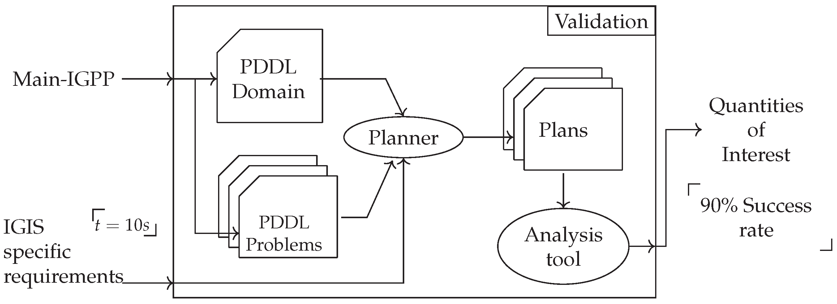
3.3. Validation Methodology for a Main Instance of the Generic Planning Problem (IGPP)

AI task planning used as a high-level control strategy can deliver the required autonomy and flexibility to an IGIS by generating plans to achieve any set goals. However, automated task planning approaches must cope in most scenarios with two challenges. The first is the large number of situational IGPPs that can be derived for an IGIS and for which a plan may be required to be generated. The second challenge is the IGIS-specific planning process constraints. Such a constraint is the planning timeout. This defines the maximal duration during which a planner must generate a plan for a planning problem.

To ensure that automated task planning can be reliably deployed in an IGIS, an extensive validation of the corresponding main IGPP is required (see Figure 6). The PDDL formulation of the main IGPP and the IGIS requirements are the inputs of our validation approach. These inputs are used to generate a representative set of PDDL planning problems for the situational IGPPs, to plan for them under the given requirements, and to analyse the results. The analysis delivers values for defined quantities of interest (QoIs). The QoIs are used to determine the overall characteristics of the main IGPP. One characteristic is the availability of planning solutions (e.g., a plan) for the selected set of situational IGPPs.

In this study, we wished to achieve the availability of planning solutions for at least $90\%$ of the situational IGPPs for the custom grippers IGPP, under the constraint of a 10-s planning timeout. Planning in the presence of, or for, humans comes with hard requirements on the available planning time, which should not be longer than a couple of seconds [39].

To better comprehend which situational IGPPs can be formulated for a main IGPP, we firstly analysed the task planning degrees of freedom for that IGPP. All possible combinations of the values that these degrees of freedom can take give the set of all possible situational IGPPs. Based on the assessment of these degrees of freedom, we have developed a task planning validation process for any IGPP.

As presented in Section 3.2.3, the PDDL domain formulation of a main IGPP has a set of fixed predicates and actions, and therefore no degrees of freedom. Furthermore, the PDDL problem formulation of a main IGPP has a set of constants $s_{0,const}$, the description of the scene $s_{0,scene}$, and the status of the process steps $s_{0,ps}$. The constants are the elements of the main IGPP that also reduce the number of degrees of freedom, as they are fixed. For example, each thingpose is attached to one or more agentposes with the at predicate and does not change during the execution of a plan. Other constants are the properties of the things (e.g., movable or placeable). Another set of fixed configurations are those of the process steps. These configurations can be defined by the user or derived from a document with instructions. An example of such a document is the manual that describes the assembly steps for a product.

In this context, the possible configurations of different agents, items, tools, and process steps are limited to only one set $s_{0,const}$, specific for the main IGPP and all its situational IGPPs. However, other aspects can be varied. These aspects are, for example, the distribution of the items and tools at the thingposes or the distribution of the agents at the agentposes. The list of already-executed process steps, as well the list with the process steps to be carried out (e.g., the goals), can also be varied. Therefore, different sets $s_{0,scene}$, $s_{0,ps}$, and g can be formulated for the main IGPP. The scenes, the statuses of the process steps, and the goals are the degrees of freedom of the main IGPP that spawn the set of possible situational IGPPs considered in our validation approach.

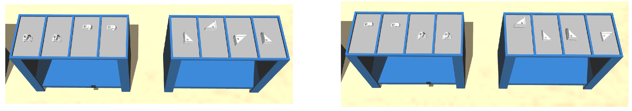
3.3.1. Scene Initial States for a Main Instance of the Generic Planning Problem (IGPP)

As mentioned in Section 3.2.3, a scene for an IGIS is a specific distribution of the things to the thingposes and of the agents to the agentposes. Therefore, more scenes are possible for an IGIS. To reduce the number of possible distributions and to guarantee that only distributions that make logical and physical sense are selected, our validation methodology splits the things, agents, and poses sets into subsets and introduces mappings between these sets. The splitting procedures and the mappings are also dependent on the selected IGIS.

To better understand the approaches introduced above, an example is given for a simplified IGIS. The following sets of items and thingposes are given:

$$\begin{array}{cc}\hfill I =& \{connector\_i,corner\_i|i\in \{1,\dots ,4\}\}\hfill \\ \hfill T =& \{itembench\_i\_thingpose\_j|i\in \{1,2\},j\in \{1,\dots ,4\}\}.\hfill \end{array}$$

(2)

These two sets are split as follows:

$$\begin{array}{cc}\hfill I_1=& \{connector\_i|i\in \{1,\dots ,4\}\};I_2=\{corner\_i|i\in \{1,\dots ,4\}\}\hfill \\ \hfill T_1=& \{itembench\_\mathit{1}\_thingpose\_j|j\in \{1,\dots ,4\}\}\hfill \\ \hfill T_2=& \{itembench\_\mathit{2}\_thingpose\_j|j\in \{1,\dots ,4\}\}.\hfill \end{array}$$

(3)

The elements of set $I_1$ are mapped to the elements of set $T_1$ and the elements of set $I_2$ to the elements of set $T_2$. These splitting and mapping procedures guarantee that the physical and logical constraints of the IGIS are satisfied. In the example, the connectors can be placed only on itembench_1, and the corners can be placed only on itembench_2 (see Figure 7).

In the next step, the mapping functions between all subsets must be defined. One possibility would be to determine all combinations of allowed assignments of things and agents to poses. However, the number of these assignments increases exponentially with the number of things, agents, or poses. For the custom grippers IGIS, the number of possible configurations is still extremely high. For this reason, the mapping procedures are based on a random method, in which each thing and agent is randomly allocated to only one pose. This mapping approach has thus only one degree of freedom: the number of randomly generated scenes $n_{scene}$. This number corresponds to the number of scene initial states and it spawns a subset of all situational IGPPs for the selected main IGPP. Finally, each scene is translated into PDDL with at grounded predicates, resulting in a set $s_{0,scene}$, which is part of an initial state $s_0$.

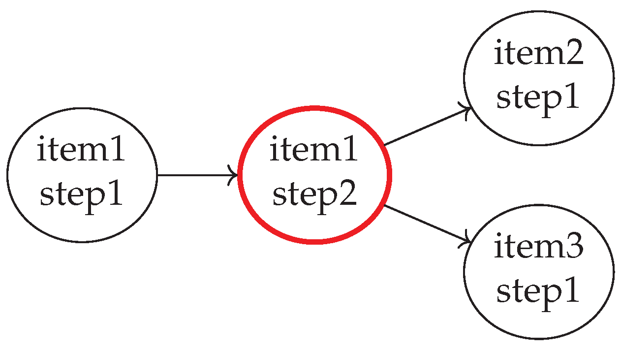
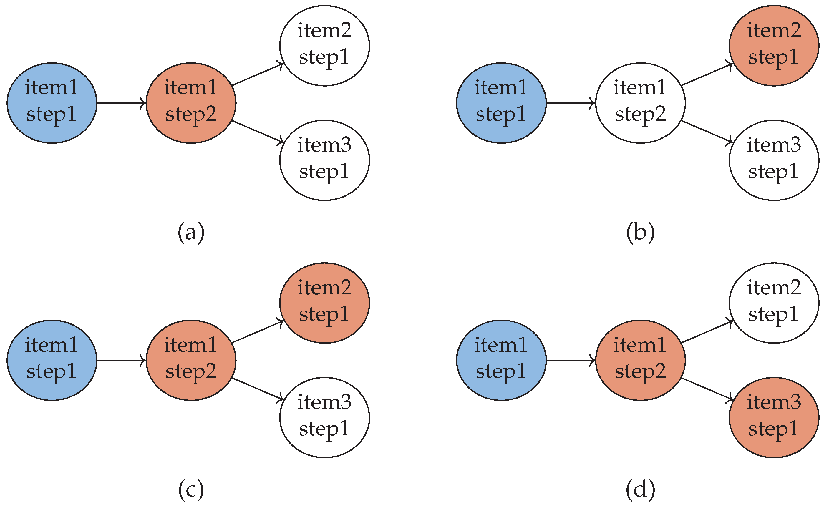
3.3.2. Process Steps Initial States and Process Steps Goals for a Main Instance of the Generic Planning Problem (IGPP)

This subsection presents our methodology used to determine allowed process steps initial states and process steps goals for a given main IGPP. These states are the second type of degrees of freedom that spawn the set of situational IGPPs.

At the beginning, the subsets $s_{0,const}$ and $s_{0,ps}$ from the PDDL problem formulation of the main IGPP are identified. From these, three types of information are extracted and used in the validation method: the configuration of all process steps, the start process steps of the processing chain $s{t}_{ps}$, and the process steps that must be finished by the end of the processing chain $f{i}_{ps}$.

The configuration of the process steps is interpreted from the grounding predicates from set $s_{0,const}$ of the PDDL formulation of the main IGPP and further encoded in a graph structure that allows an easy representation of these process steps and their dependencies.

Definition 3.

A directed simple graph $G=(V,E,\varphi )$, where V is the set of vertices, E the set of edges, and $\varphi :E\to \left\{(x,y)\right|(x,y)\in V^2,x\ne y\}$ a function that maps each edge to an ordered pair of vertices.

Definition 4.

A dependency graph $DG=(\tilde{V},\tilde{E},\tilde{\varphi })$ for a main IGPP is a directed simple graph. Each vertex $v\in \tilde{V}$ is generated by parsing the first two parameters of the grounded predicates process_step_NAME from $s_{0,const}$ in form of itemX_stepNR. Each edge $e\in \tilde{E}$ and the function $\tilde{\varphi }$ are defined by parsing the pairs of each two consecutive parameters of the grounded predicates process_step_precedence_typeX. The first pair corresponds to the parent vertex, while the following pairs correspond to the child vertices connected to that parent vertex.

Each vertex $v\in \tilde{V}$ can have zero, one, or more output edges $e\in \tilde{E}$ and has at least one input edge. Vertices with more than one output edge enable the parallel execution of process steps after their execution, while vertices with more than one input edge transform the parallel execution to a sequential one.

The configuration of the process steps as presented in Listing 11 is translated in the DG from Figure 8, while Appendix A shows the dependency graph of the custom gripper main IGPP.

Listing 11. Excert from the PDDL problem formulation for a simple IGPP.

  1 (:init

  2 (process_step_connect item1 step1 workbench2_thingpose1)

  3 (process_step_precedence_type1 item1 step1 item1 step2)

  4 (process_step_connect item1 step2 workbench2_thingpose1)

  5 (process_step_precedence_type1 item1 step2 item2 step1)

  6 (process_step_precedence_type1 item1 step2 item3 step1)

  7 (process_step_connect item2 step1 workbench2_thingpose1)

  8 (process_step_connect item3 step2 workbench2_thingpose1)

  9 (process_step_todo item1 step1) …)

10 (:goal (and

11 (process_step_done item1 step2)

12 (process_step_done item2 step1)

13 (process_step_done item3 step1)…))

Furthermore, the start-process-steps set $s{t}_{ps}$ and the finish-process-step set $f{i}_{ps}$ also contain elements in the form itemX_stepNR. The elements of set $s{t}_{ps}$ are obtained by parsing the first two parameters of the grounded predicates process_step_todo from the initial-state sub-set $s_{0,ps}$. The elements of set $f{i}_{ps}$ are obtained by parsing the first two parameters of the grounded predicates process_step_done from the goals set g. For the example presented in Listing 11, the two sets have the following elements:

$$\begin{array}{cc}\hfill s{t}_{ps}=& \{item\mathit{1}\_step\mathit{1}\}\hfill \\ \hfill f{i}_{ps}=& \{item\mathit{1}\_step\mathit{1},item\mathit{1}\_step\mathit{2},item\mathit{2}\_step\mathit{1},item\mathit{3}\_step\mathit{1}\}.\hfill \end{array}$$

(4)

Using the definition of the dependency graph and of the sets $s{t}_{ps}$ and $f{i}_{ps}$, the validation methodology can be introduced. In a simplified case, a possible validation approach for the IGPP checks if a plan can be generated only for the main IGPP. The main IGPP has in its initial state corresponding grounded predicates for all the elements of the set $s{t}_{ps}$, and in its goals, grounded predicates for all elements of the set $f{i}_{ps}$. This simplified approach is not complete enough for the validation of the main IGPP for two reasons. First, the configuration and dependencies of all process steps can be so complex that the selected planning problem cannot be solved within the set deadline. This is the case, for example, when the set $f{i}_{ps}$ has many elements. The second reason is related to the scenarios considered in this work. Especially due to the involvement of human actors, it is possible that during the execution of the process steps, errors occur and new plans must be generated. These plans must be computed from new initial states that imply new start-process-steps sets ${\widetilde{st}}_{ps,i}$. The sets ${\widetilde{st}}_{ps,i}$ are different from the original set $s{t}_{ps}$, where nothing has yet happened.

Each of the two issues presented above requires a special approach. The first challenge, which is related to the complexity of a main IGPP, can be tackled by selecting only a sub-set of all process steps that should be planned for in a planning iteration. Subsets ${\widetilde{fi}}_{ps,j}$ with cardinality $n_{ps}$ (where $n_{ps}\le \left|f{i}_{ps}\right|$) can be determined for the original set $f{i}_{ps}$. A sub-set ${\widetilde{fi}}_{ps,j}$ with $n_{ps}$ process steps to be carried out need not necessarily be determined with respect to the original start-process-steps set $s{t}_{ps}$. Such a sub-set can also be defined relative to other start-process-steps sets ${\widetilde{st}}_{ps,i}$. The sets ${\widetilde{st}}_{ps,i}$ are obtained, for example, when an error occurs during execution and a new plan from a new initial state is required.

Figure 8 presents an example of start-process-steps and finish-process-steps sets. For the original initial state $s_0$, ${\widetilde{st}}_{ps,1}=s{t}_{ps}$ holds, while for the original goals set g, $f{i}_{ps}$ holds as in Equation (4). We assume that our planner cannot find a plan in the given timeout period if the corresponding planning problem has more than three process steps goals. Therefore, $n_{ps}=3$, and the new set of finish process steps can be defined as ${\widetilde{fi}}_{ps,1}=\{item\mathit{1}\_step\mathit{1},item\mathit{1}\_step\mathit{2},item\mathit{3}\_step\mathit{1}\}$. We also assume that during the execution of item1_step2, an error occurs and a new plan must be generated. The new initial state $s_{0,2}$ is different from the original initial state $s_0$ because the first step has already been executed. In this case, ${\widetilde{st}}_{ps,2}=\{item\mathit{1}\_step\mathit{2}\}$ holds. The set of finish process steps ${\widetilde{fi}}_{ps,2}=f{i}_{ps}$ relative to the new start-process-steps set then contains all process steps, while the first process step is already executed. The planner should find a plan that does not modify the status of the first process step and guarantees that the other $n_{ps}=3$ will also be reached. This is a simplified example, but it shows that a complete validation method must consider all possible initial states and sets of goals for the given main IGPP corresponding to further situational IGPPs. Thus, all start-process-steps sets ${\widetilde{st}}_{ps,i}$ and finish-process-steps sets ${\widetilde{fi}}_{ps,j}$, where the latter sets have $n_{ps}$ elements more than the former, must be considered in the validation method. The technicalities of determining the sets ${\widetilde{st}}_{ps,i}$ and ${\widetilde{fs}}_{ps,j}$, and their formulation in PDDL are presented in the following.

Many initial states can be derived for a main IGPP. However, not all such initial states are allowed. To determine the set of start-process-steps sets $S{T}_{ps}=\left\{{\widetilde{st}}_{ps,i}\right\}$ for the allowed initial states, the information contained in the DG is used. An allowed start-process-steps set ${\widetilde{st}}_{ps,i}$ represents the information encoded in the leaves of a special dependency sub-graph DsG of the DG.

Definition 5.

A dependency sub-graph $DsG=(\overline{V},\overline{E},\overline{\varphi })$ is a sub-graph of a $DG=(\tilde{V},\tilde{E},\tilde{\varphi })$ that contain all vertices $v\in \tilde{V}$ of all direct paths $dp$ between the $start\in \tilde{V}$ vertex and its leaves. More formally, $\overline{V}=\{x\in \tilde{V}|x\in \left\{dp\right\},dp=(start,\dots ,y)fory\in \overline{V}\wedge children\left(y\right)=\varnothing \}$; $\overline{E}=\{(x,y)|(x,y)\in \tilde{E}\wedge x,y\in \overline{V}\}$; $\overline{\varphi }:\overline{E}\to \{(x,y)|(x,y)\in {\overline{V}}^2,x\ne y\}$.

This condition ensures that all process steps prior to those from the leaves of a DsG are already finished. For the example from Figure 8, if item1_step2 should be part of an initial state, the vertices item1_step1 and item1_step2 must be vertices in the corresponding DsG.

Algorithm 1 presents the steps for computing the DsGs of the DG that correspond to the given main IGPP. In a first step, the set of dependency sub-graphs is initialized with the first DsG containing only one element: the start vertex (line 1). In addition, the vertices of the input DG are ordered according to the breadth-first search (bfs) approach (line 2). The main for loop (lines 3–16) iterates over all bfs-ordered vertices. For each vertex, its children are obtained as in the original DG (line 4), and sets with all possible combinations of these children are determined (line 5). The second for loop iterates over the already-generated $DsGs$ and determines the vertices for each of them (line 7). Then, it is checked whether the bsf_vertex from the main for loop is among the vertices of the actual DsG (line 8). If so, new $DsGs$ are generated by extending the actual DsG with the combinations of the bsf-vertex’s children (lines 9–13). A bfs was used to order the vertices of the DG, because with this ordering, the expansion process of the sub-graphs is easier to follow. Indeed, any list with all vertices of the DG could have been used. The leaves of each of the obtained $DsGs$ are the elements of a start-process-steps set ${\widetilde{st}}_{ps,i}\in S{T}_{ps}$.

Algorithm 1: Algorithm for generating dependency sub-graphs (DsGs) from a DG.

The finish-process-steps sets ${\widetilde{fi}}_{ps}\in F{I}_{ps}$ are computed from the set of start-process-steps sets $S{T}_{ps}$, as presented in Algorithm 2. A finish-process-steps set ${\widetilde{fi}}_{ps}$ is also an element of $S{T}_{ps}$, because the same conditions related to the dependencies between the process steps must hold. In this context, the developed algorithm uses each two different elements of $S{T}_{ps}$ (e.g., sets) and checks if the second element can be selected as a finish-process-steps set for the first one as a start-process-steps set. This condition holds if the number of elements of ${\widetilde{st}}_{ps,j}\in S{T}_{ps}$ is larger than the number of elements of ${\widetilde{st}}_{ps,i}\in S{T}_{ps}$ by $n_{ps}$, and all elements of ${\widetilde{st}}_{ps,i}$ are also elements of ${\widetilde{st}}_{ps,j}$ (line 5). Two remarks are important at this point. First, for each start-process-steps set ${\widetilde{st}}_{ps,i}$ more finish-process-steps sets ${\widetilde{fi}}_{ps,j}\in F{I}_{ps,i}$ that fulfil the conditions are possible. Second, the conditions from line 5 guarantee that the dependencies between the process steps are considered. These dependencies are fulfilled if, from the process steps of set ${\widetilde{st}}_{ps,i}$ only the process steps from set ${\widetilde{fi}}_{ps,j}$ can be reached (second condition). Figure 9 presents four cases of allowed and not allowed pairs of start-process-steps and finish-process-steps sets for the main IGPP partly described in Listing 11.

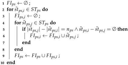
Algorithm 2: Algorithm for generating finish-process-steps sets for a given set of start-process-steps sets.

Finally, the determined start-process-steps sets $S{T}_{ps}$ and the finish-process-steps sets $F{I}_{ps}$ are translated into PDDL commands. This translation is the inverse of the process presented at the beginning of this subsection. The elements ${\widetilde{st}}_{ps,i}\in S{T}_{ps}$ are split into two parameters: item and step. These parameters are inserted in the process_step_done PDDL commands and integrated into the subset $s_{0,ps}$ of the initial state $s_0$. The elements of a set ${\widetilde{fi}}_{ps,j}\in F{I}_{ps,i}$ that are not elements of the corresponding set ${\widetilde{st}}_{ps,i}$ are then translated into parameters for process_step_todo PDDL commands and integrated into the goals list g.

Putting everything together, we have proposed a validation approach for any main IGPP. The aim of our methodology is to generate a set of representative situational IGPPs for the given main IGPP by varying allowed scenes, process steps initial states, and process steps goals. In the next subsection, plans are computed for the obtained situational IGPPs, and the results are interpreted.

4. Results

This section presents the results of the analysis carried out on the custom grippers main IGPP. The inputs of this analysis were the situational IGPPs with their variations with respect to the scenes and process steps. For each of these situational IGPPs, plans were computed with a timeout of 10 s. Four different automated planners were deployed for each situational IGPP: popf [40], optic [41], tflap [42], and tfd [43]. For each obtained plan, three characteristics were derived:

• solvability: Whether a solution was found in the timeout period of 10 s;
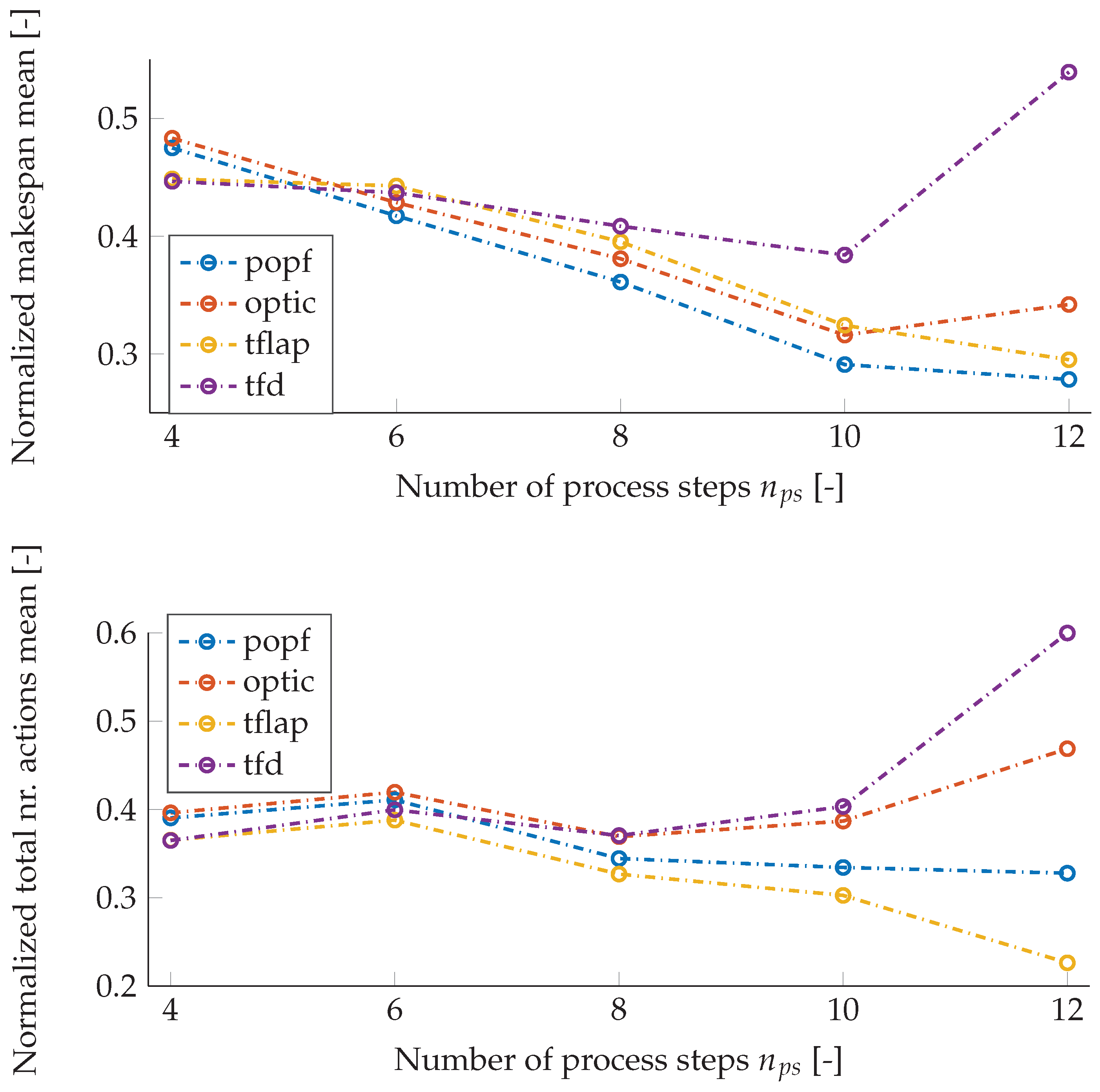
• makespan: If a solution was found, the makespan (latest end time of the actions from a plan) of the plan was determined;
• nr_actions: If a solution was found, the number of actions of that plan was determined.

The three characteristics of each plan were analysed in a context (e.g., over all situational IGPPs with a specific number of process steps $n_{ps}$) and quantities of interest (QoIs) were determined. The QoIs for a set of plans were:

• QoI 1: Percentage of solved situational IGPPs;
• QoI 2: The mean of the plans’ makespans;
• QoI 3: The mean of the plans’ numbers of actions.

For the custom grippers main IGPP, $n_{scene}=250$ scenes were generated. Corresponding to the DG from Appendix A, $141+101+55+27+14=338$ pairs of start-process-steps sets and finish-process-steps sets, for different $n_{ps}\in \{4,6,8,10,12\}$, were created. By combining all scenes with all process steps configurations, 84,500 situational IGPPs formulated in PDDL were obtained. Each of the obtained situational IGPPs was solved with the four planners, resulting in a total of 338,000 runs.

The first computed QoI was the percentage of solved situational IGPPs. The percentage was computed over all scenes and variations in the initial and goal states, for each $n_{ps}$ value, and for each of the four planners. The results are presented in

Table 1. Percentage of solved situational IGPPs for the four different planners and the five different values of $n_{ps}$.

planner|${\mathit{n}}_{\mathit{ps}}$	4	6	8	10	12
popf	$84.1\%$	$84.4\%$	$77.6\%$	$66.8\%$	$64.6\%$
optic	$90.2\%$	$95.0\%$	$89.8\%$	$84.7\%$	$88.1\%$
tflap	$97.2\%$	$94.2\%$	$79.2\%$	$44.0\%$	$6.3\%$
tfd	$98.8\%$	$94.3\%$	$93.3\%$	$93.3\%$	$94.3\%$

.

The results show that the tfd planner managed to solve more than $90\%$ of the situational IGPPs corresponding to each different number of goals. The optic planner delivered a success rate greater than $84\%$ in finding a plan in all sets of situational IGPPs for different $n_{ps}$ values.

The next two QoIs were the mean of the plans’ makespans and the mean of the plans’ numbers of actions, over a subset of all situational IGPPs. This subset contained all situational IGPPs for all scenes, for a given $n_{ps}$, and a given planner. The makespan and nr_actions characteristics of the obtained plans were normalized, to enable a comparison of the results of the different subsets (e.g., different $n_{ps}$ values and planners). For the normalization of the data, the min-max approach was used:

$$x_{norm}=\frac{x-x_{min}}{x_{max}-x_{min}}.$$

(5)

Here, $x_{min}$ and $x_{max}$ are computed for the makespans and numbers of actions of all situational IGPP variations corresponding to one $n_{ps}$ value but independent of the planner used to solve them.

Figure 10 depicts the obtained results. The planners popf and optic computed, in most cases, the plans with the lowest mean makespan. However, the planners tflap and popf generated the plans with the lowest mean numbers of actions for almost all $n_{ps}$ values. The planner tfd usually generated plans with the highest mean makespans and the highest mean numbers of actions.

5. Discussion and Conclusions

The main results of this work were the description of the generic industrial scenario with its instances IGIS, the formulation of the generic planning problem and of one instance, the custom grippers IGPP, and the validation results for the selected IGPP.

The results showed that the GIS derived from independent scenarios described in related works could be easily configured for a new scenario, i.e., the custom grippers scenario. Furthermore, the generic planning problem originally formulated for the GIS could also be easily adapted for the custom grippers IGPP. For the PDDL formulation of the IGPP, only changes in the naming of the PDDL artefacts and in the problem files were required. No further modelling was necessary.

Using the validation methods presented in Section 3.3, we showed that the PDDL formulation of the main IGPP could guarantee a success rate of $90\%$ for generating plans for a high number of situational IGPPs. These results demonstrate that AI planning approaches (e.g., temporal planning) formulated in PDDL can be used in real-world IGIS. Automated planning approaches are already deployed as a high-level control strategy in simulated or real industrial scenarios [1,4,44]; however, no generic planning problems and corresponding validation methodologies for them have yet been developed.

Automated planners for planning problems formulated in PDDL are usually compared one to another based on a set of standard planning domains and problems (https://ipc2018-classical.bitbucket.io/domains.html (accessed on 17 February 2022)). None of these planning problems is formulated for a generic industrial scenario. Some studies from the literature present planning problems, but only for specific scenarios [1,45]. Therefore, no suggestions regarding a suitable temporal planner are available in the literature that can solve planning problems formulated for such scenarios. Further results of our work showed that the temporal planners optic and tfd were suitable temporal planners for the IGPP formulation of the gripper scenario, when plans must be generated within a deadline of 10 s and the planning problems have $n_{ps}\in \{4,6,8\}$ process steps. For planning problems with $n_{ps}>8$, no concrete statements can be formulated.

The work conducted so far shows the theoretical advantage of deploying automated task planning methodologies based on the GIS and the PDDL formulation of the GPP as high-level control approaches for industrial scenarios with mobile manipulators. In future work, we wish to transfer these results to simulated and real scenarios, by executing the plans generated for the different situational IGPPs. A further validation methodology with corresponding QoIs will be defined. This will focus on the execution times and on the re-plan rates.

In conclusion, this work introduced a generic industrial scenario, a generic planning problem formulated in PDDL, and a validation methodology for instances of the GPP. These models and approaches can be used as a starting point for deploying automated planning approaches in any further industrial scenario with mobile manipulators.

References

1. Bezrucav, S.O.; Corves, B. Improved AI Planning for Cooperating Teams of Humans and Robots. In Proceedings of the Workshop on Planning and Robotics (PlanRob) at the International Conference on Automated Planning and Scheduling (ICAPS), Nancy, France, 26–30 October 2020. [Google Scholar] [CrossRef]
2. Wally, B.; Vyskocil, J.; Novak, P.; Huemer, C.; Sindelar, R.; Kadera, P.; Mazak, A.; Wimmer, M. Production Planning with IEC 62264 and PDDL. In Proceedings of the 17th International Conference on Industrial Informatics (INDIN), Helsinki, Finland, 22–25 July 2019; pp. 492–499. [Google Scholar] [CrossRef]
3. Kootbally, Z.; Schlenoff, C.; Lawler, C.; Kramer, T.; Gupta, S.K. Towards robust assembly with knowledge representation for the planning domain definition language (PDDL). Robot. Comput.-Integr. Manuf. 2015, 33, 42–55. [Google Scholar] [CrossRef]
4. Foderaro, E.; Cesta, A.; Umbrico, A.; Orlandini, A. Simplifying the AI Planning modeling for Human-Robot Collaboration. In Proceedings of the 30th IEEE International Conference on Robot & Human Interactive Communication (RO-MAN), Vancouver, BC, Canada, 8–12 August 2021; pp. 1011–1016. [Google Scholar] [CrossRef]
5. Ghallab, M.; Dana, N.; Traverso, P. Automated Planning and Acting; Cambridge University Press: Cambridge, UK, 2016. [Google Scholar]
6. Iovino, M.; Scukins, E.; Styrud, J.; Ögren, P.; Smith, C. A Survey of Behavior Trees in Robotics and AI. arXiv 2020, arXiv:2005.05842. [Google Scholar]
7. RoboCup Federation. RoboCup Logistics League. Available online: https://ll.robocup.org/home/ (accessed on 1 February 2022).
8. Zug, S.; Niemueller, T.; Hochgeschwender, N.; Seidensticker, K.; Seidel, M.; Friedrich, T.; Neumann, T.; Karras, U.; Kraetzschmar, G.K.; Alexander, F. An Integration Challenge to Bridge the Gap Among Industry-Inspired RoboCup Leagues. In RoboCup 2016: Robot World Cup XX; Behnke, S., Sheh, R., Sarıel, S., Lee, D.D., Eds.; Number 9776; Springer International Publishing: Berlin/Heidelberg, Germany, 2017; pp. 157–168. [Google Scholar]
9. Norouzi, A.; Zug, S.; Martin, J.; Nair, D.; Steup, C. RoboCup@Work 2020—Rulebook. 2020. Available online: https://robocup-lyontech.github.io/assets/pdf/Rulebook_robocup_2020-11-25.pdf (accessed on 1 February 2022).
10. Kraetzschmar, G.K.; Hochgeschwender, N.; Nowak, W.; Hegger, F.; Schneider, S.; Dwiputra, R.; Berghofer, J.; Bischoff, R. RoboCup@Work: Competing for the Factory of the Future. In RoboCup 2014: Robot World Cup XVIII; Bianchi, R.A.C., Akin, H.L., Ramamoorthy, S., Sugiura, K., Eds.; Springer International Publishing: Berlin/Heidelberg, Germany, 2015; pp. 171–182. [Google Scholar]
11. Martin, J.; Ammon, D.; Engelhardt, H.; Fink, T.; Gramß, F.; Gsell, A.; Heigl, D.; Koch, P.; Masannek, M. Team Description Paper—Team AutonOHM. 2016. Available online: https://www.th-nuernberg.de/fileadmin/fakultaeten/efi/efi_bilder/Labore/RoboCup/AutonOHM%40Work_Team_Description_Paper-TDP-2016.pdf (accessed on 1 February 2022).
12. Rostami, V.; Mansournia, P.; Ghaziakar, A.; Hamzeh, A.; Jalili, F.; Dostar, M. ATISbots Team Description Paper. 2020. Available online: https://www.researchgate.net/publication/339500818_ATISbots_RoboCupWork_2020_Team_Description_Paper (accessed on 1 February 2022).
13. Katz, M.; Hoffmann, J. Pushing the Limits of Partial Delete Relaxation: Red-Black DAG Heuristics. 2014. Available online: https://www.robocup2017.org/file/symposium/atWork/tdp_b-it-bots_atwork_2017.pdf (accessed on 1 February 2022).
14. Jandt, T.; Kulkarni, P.; Mayoral, J.C.; Nair, D.; Senga, B.N.; Thoduka, S.; Awaad, I.; Hochgeschwender, N.; Schneider, S.; Kraetzschmar, G.K. b-it-bots Team Description Paper. 2017. Available online: https://fai.cs.uni-saarland.de/katz/papers/ipc2014a.pdf (accessed on 1 February 2022).
15. Steup, C.; Seidel, M.; Busse, P.; Harder, N.; Hoyer, L.; Jorges, G.; Jose, J.C.; Kopton, J.; Koring, A.; Labitzke, F.; et al. Team Description Paper robOTTO. 2019. Available online: https://www.robotto.ovgu.de/robotto_media/Downloads/TDPs/tdp_robotto_2019.pdf (accessed on 1 February 2022).
16. Festo. Robotino—Forschen und Lernen mit Robotern. Available online: https://www.festo-didactic.com/int-en/highlights/qualification-for-industry-4.0/robotino-4/?fbid=aW50LmVuLjU1Ny4xNy4xMC44MjU1LjQ1NTg (accessed on 1 February 2022).
17. Vincent, C.; Deppe, C.; Gomaa, M.; Hofmann, T.; Karras, U.; Niemueller, T.; Rohr, A.; Ulz, T. The RoboCup Logistics League. Available online: https://github.com/robocup-logistics/rcll-rulebook/releases/download/2019/rulebook2019.pdf (accessed on 1 February 2022).
18. Kohout, P.; de Bortoli, M.; Ludwiger, J.; Ulz, T.; Steinbauer, G. A multi-robot architecture for the RoboCup Logistics League. Elektrotech. Informationstech. 2020, 137, 291–296. [Google Scholar] [CrossRef]
19. Hofmann, T.; Limpert, N.; Mataré, V.; Schönitz, S.; Niemueller, T.; Ferrein, A.; Lakemeyer, G. The Carologistics RoboCup Logistics Team 2018. 2018. Available online: https://ll.robocup.org/wp-content/uploads/2018/11/carologistics-2018-tdp.pdf (accessed on 1 February 2022).
20. Niemueller, T.; Hofmann, T.; Lakemeyer, G. Goal Reasoning in the CLIPS Executive for Integrated Planning and Execution. In Proceedings of the Twenty-Ninth International Conference on Automated Planning and Scheduling, Berkeley, CA, USA, 11–15 July 2019; Smith, D.E., Srivastava, S., Eds.; AAAI Press: Palo Alto, CA, USA, 2019; pp. 754–763. [Google Scholar]
21. Steup, C.; Seidel, M.; Bartsch, L.; Brockhage, I.; Harder, N.; Harriehausen, N.; Jorges, G.; Klobertanz, A.; Koring, A.; Labitzke, F.; et al. Team Description Paper robOTTO. 2020. Available online: https://www.robotto.ovgu.de/robotto_media/Downloads/TDPs/tdp_robotto_2020.pdf (accessed on 1 February 2022).
22. Scholz, M.; Sessner, J.; Eith, F.; Zwingel, M.; Merbele, S.; Gruendel, L.; Garbe, V.; Reitelshoefer, S.; Franke, J. The ER-Force RoboCup Logistics League Team 2018. 2018. Available online: https://ll.robocup.org/wp-content/uploads/2018/11/TDP-ER-Force-LogisticsLeague-2018.pdf (accessed on 1 February 2022).
23. Rohr, A.; Brandenberger, S. Description of Team Solidus 2018. 2018. Available online: https://ll.robocup.org/wp-content/uploads/2018/11/Team_Solidus_TDP_2018_eng.pdf (accessed on 1 February 2022).
24. De Bortoli, M.; Stenbauer, G. The RoboCup Logistics League from a Planning Perspective. In Proceedings of the Workshop on Planning and Robotics (PlanRob) at International Conference on Automated Planning and Scheduling (ICAPS), Nancy, France, 26–20 October 2020. [Google Scholar]
25. Niemueller, T.; Karpas, E.; Vaquero, T.; Timmons, E. Planning and Execution Competition for Logistics Robots in Simulation. Available online: http://www.robocup-logistics.org/sim-comp/logrobcomp-rules2017-v2.pdf?attredirects=0 (accessed on 1 February 2022).
26. RoboCup Logistics League. Planning and Execution Competition for Logistics Robots in Simulation. Available online: http://www.robocup-logistics.org/sim-comp (accessed on 1 February 2022).
27. Schäpers, B.; Niemueller, T.; Lakemeyer, G. ASP-based Time-Bounded Planning for Logistics Robots. In Proceedings of the Twenty-Eighth International Conference on Automated Planning and Scheduling, Delft, The Netherlands, 24–29 June 2018; de Weerdt, M., Koenig, S., Röger, G., Spaan, M., Eds.; AAAI Press: Palo Alto, CA, USA, 2018. [Google Scholar]
28. Coles, A.; Coles, A.; Fox, M.; Long, D. Forward-Chaining Partial-Order Planning. In Proceedings of the 20th International Conference on Automated Planning and Scheduling; Brafman, R., Ed.; AAAI Press: Palo Alto, CA, USA, 2010; pp. 42–49. [Google Scholar]
29. Cashmore, M.; Fox, M.; Long, D.; Magazzeni, D.; Ridder, B.; Carrera, A.; Palomeras, N.; Hurtos, N.; Carreras, M. ROSPlan: Planning in the Robot Operating System. In Proceedings of the Twenty-Fifth International Conference on Automated Planning and Scheduling, Jerusalem, Israel, 7–11 June 2015; Brafman, R., Ed.; AAAI Press: Palo Alto, CA, USA, 2015; pp. 333–341. [Google Scholar]
30. Crosby, M.; Petrick, R.P.A.; Rovida, F.; Krueger, V. Integrating Mission and Task Planning in an Industrial Robotics Framework. In Proceedings of the Twenty-Seventh International Conference on Automated Planning and Scheduling, Pittsburgh, PA, USA, 18–23 June 2017; Barbulescu, L., Ed.; AAAI Press: Palo Alto, CA, USA, 2017; pp. 471–479. [Google Scholar]
31. Cacace, J.; Caccavale, R.; Finzi, A.; Lippiello, V. Interactive Plan Execution during Human-Robot Cooperative Manipulation. In Proceedings of the Workshop on Planning and Robotics (PlanRob) at International Conference on Automated Planning and Scheduling (ICAPS), Delft, The Netherlands, 26 June 2018; pp. 82–88. [Google Scholar]
32. Johannsmeier, L.; Haddadin, S. A Hierarchical Human-Robot Interaction-Planning Framework for Task Allocation in Collaborative Industrial Assembly Processes. IEEE Robot. Autom. Lett. 2017, 2, 41–48. [Google Scholar] [CrossRef] [Green Version]
33. Ghallab, M.; Knoblock, C.; Wilkins, D.; Barrett, A.; Christianson, D.; Friedman, M.; Kwok, C.; Golden, K.; Penberthy, S.; Smith, D.; et al. PDDL—The Planning Domain Definition Language. 1998. Available online: https://www.researchgate.net/publication/2278933_PDDL_-_The_Planning_Domain_Definition_Language (accessed on 1 February 2022).
34. Ghallab, M.; Nau, D.; Traverso, P. Automated Planning; Elsevier: Amsterdam, The Netherlands, 2004. [Google Scholar]
35. Mayer, M.C.; Orlandini, A.; Umbrico, A. A Formal Account of Planning with Flexible Timelines. In Proceedings of the 21st International Symposium on Temporal Representation and Reasoning, Verona, Italy, 8–10 September 2014; pp. 37–46. [Google Scholar] [CrossRef]
36. Cushing, W.; Subbarao Kambhampati, M.; Weld, D.S. When is temporal planning really temporal? In Proceedings of the Twentieth International Joint Conference on Artificial Intelligence, Hyderabad, India, 6–12 January 2007; Sangal, R., Mehta, H., Bagga, R.K., Eds.; AAAI Press: Palo Alto, CA, USA, 2007; pp. 1852–1859. [Google Scholar]
37. Fox, M.; Long, D. PDDL2.1: An Extension to PDDL for Expressing Temporal Planning Domains. J. Artif. Intell. Res. 2003, 20, 61–124. [Google Scholar] [CrossRef]
38. Epple, U. Grundlagen der Modellierung, Vorlesung: Modelle der Leittechnik, SS2012; RWTH Aachen: Aachen, Germany, 2013. [Google Scholar]
39. Lima, O.; Ventura, R.; Awaad, I. Integrating Classical Planning and Real Robots in Industrial and Service Robotics Domains. In Proceedings of the Workshop on Planning and Robotics (PlanRob) at International Conference on Automated Planning and Scheduling (ICAPS), Delft, The Netherlands, 26 June 2018; pp. 75–81. [Google Scholar]
40. Coles, A.; Coles, A.; Clark, A.; Gilmore, S. Cost-Sensitive Concurrent Planning Under Duration Uncertainty for Service-Level Agreements. In Proceedings of the Twenty-First International Conference on Automated Planning and Scheduling, Freiburg, Germany, 11–16 June 2011; Bacchus, F., Ed.; AAAI Press: Palo Alto, CA, USA, 2011; pp. 34–41. [Google Scholar]
41. Benton, J.; Coles, A.; Coles, A. Temporal Planning with Preferences and Time-Dependent Continuous Costs. In Proceedings of the Twenty-Second International Conference on International Conference on Automated Planning and Scheduling, ICAPS’12, Sao Paulo, Brazil, 25–29 June 2012; AAAI Press: Palo Alto, CA, USA, 2012; pp. 2–10. [Google Scholar]
42. Sapena, O.; Marzal, E.; Onaindia, E. TFLAP: A Temporal Forward Partial-Order Planner. 2018. Available online: https://ipc2018-temporal.bitbucket.io/planner-abstracts/team2.pdf (accessed on 1 February 2022).
43. Eyerich, P.; Mattmüller, R.; Röger, G. Using the Context-enhanced Additive Heuristic for Temporal and Numeric Planning. In Proceedings of the Nineteenth International Conference on Automated Planning and Scheduling, Thessaloniki, Greece, 19–23 September 2009; Gerevini, A., Howe, H., Cesta, A., Refanidis, R., Eds.; ICAPS and International Conference on Automated Planning and Scheduling. AAAI Press: Palo Alto, CA, USA, 2009; pp. 114–121. [Google Scholar]
44. Orlandini, A.; Cialdea Mayer, M.; Umbrico, A.; Cesta, A. Design of Timeline-Based Planning Systems for Safe Human-Robot Collaboration. In Knowledge Engineering Tools and Techniques for AI Planning; Vallati, M., Kitchin, D., Eds.; Springer International Publishing: Berlin/Heidelberg, Germany, 2020; pp. 231–248. [Google Scholar] [CrossRef]
45. Bezrucav, S.O.; Kaiser, M.; Corves, B. Case Study: AI Task Planning Setup for an Industrial Scenario with Mobile Manipulators. In Proceedings of the Scheduling and Planning Applications Workshop of The Thirty-First International Conference on Automated Planning and Scheduling, Guangzhou, China, 2–13 August 2021. [Google Scholar] [CrossRef]
Figure 1. Examples of simulated (first two agents) and real (last two agents) mobile manipulators.
Applsci 12 02319 g001
Figure 2. A description of the process steps on the different items of product A.
Applsci 12 02319 g002
Figure 3. The relations between the process steps on the different items of product A.
Applsci 12 02319 g003
Figure 4. Three states at the beginning of, during, and at the end of the execution of the navigate action and the corresponding values of the grounded predicates describing these states.
Applsci 12 02319 g004
Figure 5. The custom grippers instance of the generic industrial scenario.
Applsci 12 02319 g005
Figure 6. Validation methodology for a main IGPP.
Applsci 12 02319 g006
Figure 7. Sub-areas of two scenes of the custom gripper IGIS.
Applsci 12 02319 g007
Figure 8. Dependency graph (DG) for a simple IGPP.
Applsci 12 02319 g008
Figure 9. The four sub-figures present combinations of start-process-steps sets (blue vertices) and finish-process-steps sets (red vertices): (a) is an allowed combination of an s t ˜ p s , i and an f i ˜ p s , j , where n p s = 1 ; (b) is a not-allowed combination of an s t ˜ p s , i and an f i ˜ p s , j ; (c,d) are two allowed combinations of an s t ˜ p s , i and an f i ˜ p s , j , where n p s = 2 .
Applsci 12 02319 g009
Figure 10. Normalized means of plans’ makespans and numbers of actions for the four planners and different n p s values.
Applsci 12 02319 g010