
Hough Transform Sensitivity Factor Calculation Model Applied to the Analysis of Acne Vulgaris Skin Lesions

 ,
,  and
and 
Abstract
:1. Introduction
2. Background
2.1. Basic Idea of Circular Hough Transform Function (CHT)
2.2. CHT in Matlab
3. Material and Methods

| Trial 1 | SfactorR | 0.81 | 0.82 | 0.83 | 0.84 | 0.85 | 0.86 | 0.87 | 0.88 | 0.89 | 0.9 | 0.91 | 0.92 | 0.93 | 0.94 | 0.95 |
| NP | - | 403 | 471 | 549 | 605 | 657 | 708 | 754 | 787 | 877 | 945 | 966 | 1001 | 1087 | 1182 | |
| W | - | 0.460 | 0.583 | 0.752 | 0.898 | 1.056 | 1.240 | 1.436 | 1.600 | 2.182 | 2.829 | 3.086 | 3.601 | 5.661 | 12.190 | |
| R2 | - | - | 94.10 | 95.26 | 96.46 | 97.62 | 98.64 | 99.39 | 99.56 | 98.16 | 96.06 | 94.74 | - | - | - | |
| Signif. | - | - | X | X | X | X |  | | | | | X | - | - | - |
, all the p-values < 0.05 then the model is significant.3.1. Statistical Analysis
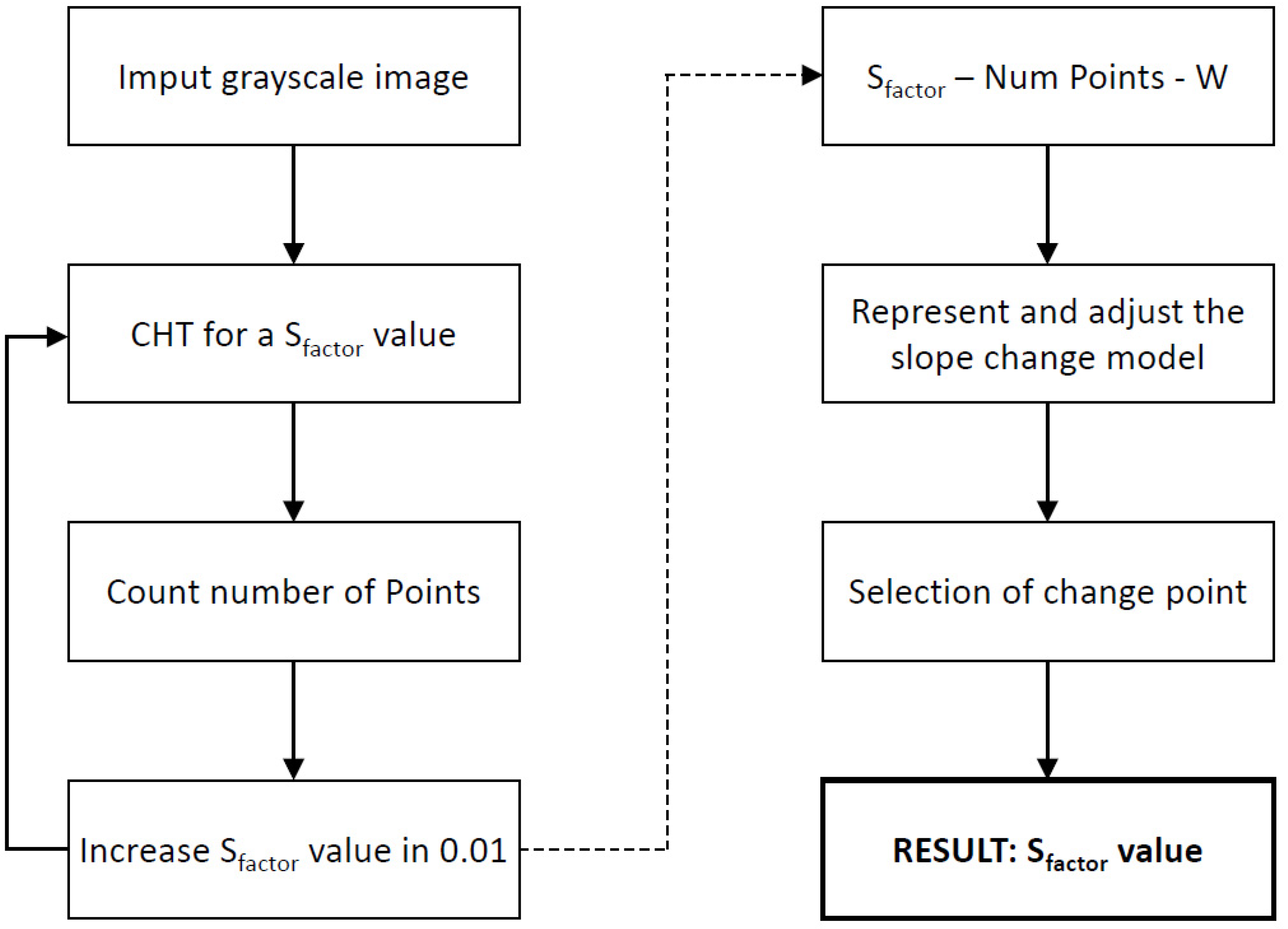
3.2. Flowchart
4. Results and Discussion
- -
- An increase in the final precision in the counting of points by applying CHT.
- -
- Being an objective method, it allows the results of the algorithm to be compared with other point counting algorithms.
5. Conclusions
Author Contributions
Funding
Informed Consent Statement
Acknowledgments
Conflicts of Interest
References
- Fernández-Guarino, M.; Harto, A.; Sánchez-Ronco, M.; Pérez-García, B.; Marquet, A.; Jaén, P. Retrospective, de-scriptive, observational study of treatment of multiple actinic keratoses with topical methyl aminolevulinate and red light: Results in clinical practice and correlation with fluorescence imaging. Actas Dermo-Sifiliogr. 2008, 99, 779–787. [Google Scholar] [CrossRef]
- Molina, M.A.; Lopez-Rubio, E.; Luque-Baena, R.M. Blood Cell Classification Using the Hough Transform and Convolutional Neural Networks. In Trends and Advances in Information Systems and Technologies; WorldCIST’18 2018; Advances in Intelligent Systems and Computing; Springer: Cham, Switzerland, 2018; Volume 746. [Google Scholar]
- Bukowska, D.M.; Chew, A.L.; Huynj, E.; Kashani, I.; Wan, S.L.; Wang, P.M.; Chen, F.K. Semi-automated identification of cones in human retina using circle Hough transform. Biomed. Opt. Express 2015, 6, 4676–4693. [Google Scholar] [CrossRef] [Green Version]
- Quiroz, J.M.; Delgado, P.V.V. Implementación de un Algoritmo para la Detección y Conteo de Células en Imágenes Microscópicas. Bachelor’s Thesis, Escuela Superior Politécnica del Litoral (ESPOL), Guayaquil, Ecuador, 2009. [Google Scholar]
- Cota, R.O. Reconocimiento y Cuantificación de Células de Peces en Imágenes de Cortes Histológicos; Instituto Tecnológico de La Paz: La Paz, Mexico, 2015. [Google Scholar]
- Jiménez, A.; Rydberg, N. Area of Interest Identification Using Circle Hough Transform and Outlier Removal for ELIspot and FluoroSpot Images; TFM: Barcelona, Spain, 2019. [Google Scholar]
- Memis, A.; Albayrak, S.; Bilgili, F. Femoral head detectrion in perthes MR slices with circular hough transform. In Proceedings of the 26th Signal Processing and Communications Applications Conference (SIU), Çeşme, Turkey, 2–5 May 2018; pp. 1–4. [Google Scholar] [CrossRef]
- Mohammadi, S.; Mohammadi, M.; Dehlaghi, V.; Ahmadi, A. Automatic Segmentation, Detection, and Diagnosis of Abdominal Aortic Aneurysm (AAA) Using Convolutional Neural Networks and Hough Circles Algorithm. Car-Diovasc. Eng. Technol. 2019, 10, 490–499. [Google Scholar] [CrossRef] [PubMed]
- Bosnjak, A.; Bosnjak, M.; Seijas, C. Detección de la Reflexión y Segmentación de las Imágenes Dermatológicas Uti-lizando la Técnica de ‘Level Set’. Venezuela 2016, 135–146. Available online: https://www.researchgate.net/publication/318030664_Deteccion_de_la_Reflexion_y_Segmentacion_de_las_Imagenes_Dermatologicas_Utilizando_la_Tecnica_de_%27Level_Set%27 (accessed on 25 September 2021).
- Blasco-Morente, G.; Garrido-Colmenero, C.; López, I.P.; Tercedor-Sánchez, J. Wood’ light in dermatology: An essential technique. PIEL 2014, 29, 487–494. [Google Scholar] [CrossRef]
- Elsalamony, H.A. Detecting distorted and benign blood cells using the Hough transform based on neural net-works and decision trees. In Emerging Trends in Image Processing, Computer Vision and Pattern Recognition; Morgan Kaufmann: Burlington, MA, USA, 2015; pp. 457–473. [Google Scholar]
- Mitra, J.; Chandra, A.; Halder, T. Peak Trekking of Hierarchy Mountain for the Detection of Cerebral Aneurysm using Modified Hough Circle Transform. Electron. Lett. Comput. Vis. Image Anal. 2013, 12, 57–84. [Google Scholar] [CrossRef] [Green Version]
- Malladi, R.; Sethian, J.A.; Vemuri, B.C. Shape Modeling with Front Propagation: A Level Set Approach. IEEE Trans. Pattern Anal. Mach. Intell. 1995, 17, 158–175. [Google Scholar] [CrossRef] [Green Version]
- Ahmad, T.; Tan, T.S.; Yaakub, A. Implementation of circular Hough transform on MRI images for eye globe volume estimation. Int. J. Biomed. Eng. Technol. 2020, 33, 123–133. [Google Scholar]
- Kuruganti, T.; Hirong, Q. Asymmetry analysis in breast cancer detection using thermal infrared image. Eng. Med. Biol. 2002, 2, 1155–1156. [Google Scholar]
- Schmitter, D.; Delgado-Gonzalo, R.; Unser, M. Trigonometric Interpolation Kernel to Construct Deformable Shapes for User-Interactive Applications. IEEE Signal Process. Lett. 2015, 22, 2097–2101. [Google Scholar] [CrossRef] [Green Version]
- Gao, G.; Wen, C.; Wang, H.; Xu, L. Fast Multiregion Image Segmentation Using Statistical Active Contours. IEEE Signal Process. Lett. 2017, 24, 417–421. [Google Scholar] [CrossRef]
- Raheja, J.L.; Sahu, G. Pellet Size Distribution Using Circular Hough Transform in Simulink. Am. J. Signal Process. 2012, 2, 158–161. [Google Scholar] [CrossRef]
- Mahmood, N.H.; Mansor, M.A.B. Red Blood Cells Estimations Using Hough Transform Techniqu. Signal Image Process. Int. J. (SIPIJ) 2012, 3, 53. [Google Scholar] [CrossRef]
- Xiong, W.; He, Y. Measurement of gear size parameters based on Hough transform circle segmentation. In MIPPR 2019: Remote Sensing Image Processing, Geographic Information Systems, and other Applications; International Society for Optics and Photonics: Bellingham, WA, USA, 2020. [Google Scholar]
- Bernal, J.L.; Cummins, S.; Gasparrini, A. Interrupted time series regression for the evaluation of public health interventions: A tutorial. Int. J. Epidemiol. 2017, 46, 348–355. [Google Scholar] [CrossRef] [PubMed]
- Urrea, J.P.; Ospina, E. Implementación de la transformada de hough para la detección de líneas para un siste-ma de visión de bajo nivel. Sci. Tech. Año X 2004, 1, 79–84. [Google Scholar]
- Canul-Arceo, L.; López-Martínez, J.; Narváez-Díaz, L. La función transformada circular de Hough se deriva de la transformada de Hough para la detección de objetos lineales. Program. Mat. Softw. 2015, 7, 8–13. [Google Scholar]
- Pedersen, S.J.K. Circular Hough Transform, Aalborg University, Vision, Graphics, and Interactive Systems; Aalborg University: Aalborg, Denmark, 2007. [Google Scholar]
- Peral, S. Detección de Circunferencias; Transformada de Hough; Universidad de Valladolid: Valladolid, Spain, 2002. [Google Scholar]
- Soltany, M.; Zadeh, S.T.; Pourreza, H.-R. Fast and Accurate Pupil Positioning Algoritm using Circular Hough Transform and Gray Projection. Proc. CSIT 2011, 5, 556–561. [Google Scholar]
- Kimme, C.; Ballard, D.; Sklansky, J. Finding circles by an array of accumulators. Comun. ACM 1975, 18, 120–122. [Google Scholar] [CrossRef]
- de Vegt, S. A Fast and Robust Algorithm for the Detection of Circular Pieces in A Cyber Physical System; Eindhoven University of Technology: Eindhoven, The Netherlands, 2015. [Google Scholar]
- Dai, T.; Gupta, A.; Murray, C.K.; Vrahas, M.S.; Tegos, G.P.; Hamblin, M.R. Blue light for infectious diseases: Pro-pinoibacterium acnes, Helicobacter pylori, and beyond? Drug Resist. Updates 2012, 15, 223–236. [Google Scholar] [CrossRef] [Green Version]
- Xu, D.; Yan, J.; Liu, W.; Hou, X.; Zheng, Y.; Jiang, W. Is Human Sebum the Source of Skin Follicular Ultraviolet-Induced Red Fluorescence? A cellular to Histological Study. Dermatology 2018, 234, 43–50. [Google Scholar] [CrossRef]
- Jeong, H.; Yoon, B.-J. Effective Estimation of Node-to-Node Correspondence Between Different Graphs. IEEE Signal Process. Lett. 2015, 22, 661–665. [Google Scholar] [CrossRef]


| Sfactor | Number of Points |
|---|---|
| 0.82 | 403 |
| 0.83 | 403 |
| 0.84 | 471 |
| 0.85 | 605 |
| 0.86 | 605 |
| 0.87 | 657 |
| 0.88 | 708 |
| 0.89 | 787 |
| 0.9 | 877 |
| 0.91 | 945 |
| 0.92 | 966 |
| 0.93 | 1001 |
| 0.94 | 1087 |
| 0.95 | 1182 |
| 0.96 | 1279 |
| Trial 1 | SfactorR | - | 0.82 | 0.83 | 0.84 | 0.85 | 0.86 | 0.87 | 0.88 | 0.89 | 0.9 | 0.91 | 0.92 | 0.93 | 0.94 | 0.95 |
| NP | - | 403 | 471 | 549 | 605 | 657 | 708 | 754 | 787 | 877 | 945 | 966 | 1001 | 1087 | 1182 | |
| W | - | 0.460 | 0.583 | 0.752 | 0.898 | 1.056 | 1.240 | 1.436 | 1.600 | 2.182 | 2.829 | 3.086 | 3.601 | 5.661 | 12.190 | |
| R2 | - | - | 94.10 | 95.26 | 96.46 | 97.62 | 98.64 | 99.39 | 99.56 | 98.16 | 96.06 | 94.74 | - | - | - | |
| Signif. | - | X | X | X | X | | | | | | X | - | - | - | ||
| Trial 2 | SfactorR | 0.81 | 0.82 | 0.83 | 0.84 | 0.85 | 0.86 | 0.87 | 0.88 | 0.89 | 0.9 | 0.91 | - | - | - | - |
| NP | 187 | 205 | 220 | 236 | 256 | 285 | 320 | 378 | 471 | 662 | 985 | - | - | - | - | |
| W | 0.234 | 0.263 | 0.288 | 0.315 | 0.351 | 0.407 | 0.481 | 0.623 | 0.916 | 2.050 | - | - | - | - | - | |
| R2 | - | 91.71 | 94.03 | 96.36 | 98.30 | 99.15 | 98.15 | - | - | - | - | - | - | - | - | |
| Signif. | - | X | X | X | | | | - | - | - | - | - | - | - | - | |
| Trial 3 | SfactorR | 0.81 | 0.82 | 0.83 | 0.84 | 0.85 | 0.86 | 0.87 | 0.88 | 0.89 | 0.9 | - | - | - | - | - |
| NP | 298 | 319 | 360 | 396 | 454 | 521 | 618 | 746 | 1015 | 1271 | - | - | - | - | - | |
| W | 0.306 | 0.335 | 0.395 | 0.453 | 0.556 | 0.695 | 0.946 | 1.421 | 3.965 | - | - | - | - | - | - | |
| R2 | - | 87.09 | 90.64 | 94.23 | 97.12 | 98.81 | 96.71 | - | - | - | - | - | - | - | - | |
| Signif. | - | X | X | X | | | | - | - | - | - | - | - | - | - | |
| Trial 4 | SfactorR | - | 0.82 | 0.83 | 0.84 | 0.85 | 0.86 | 0.87 | 0.88 | 0.89 | 0.9 | 0.91 | 0.92 | 0.93 | - | - |
| NP | - | 47 | 65 | 108 | 140 | 167 | 198 | 253 | 323 | 430 | 571 | 688 | 859 | - | - | |
| W | - | 0.058 | 0.082 | 0.144 | 0.195 | 0.241 | 0.300 | 0.417 | 0.603 | 1.002 | 1.983 | 4.023 | - | - | - | |
| R2 | - | - | 93.71 | 94.74 | 96.19 | 98.00 | 99.55 | 98.59 | - | - | - | - | - | - | - | |
| Signif. | - | - | X | X | X | | | | - | - | - | - | - | - | - | |
| Trial 5 | SfactorR | - | 0.82 | 0.83 | 0.84 | 0.85 | 0.86 | 0.87 | 0.88 | 0.89 | 0.9 | 0.91 | 0.92 | 0.93 | 0.94 | 0.95 |
| NP | - | 208 | 255 | 307 | 347 | 386 | 405 | 427 | 443 | 479 | 508 | 525 | 545 | 596 | 635 | |
| W | - | 0.423 | 0.573 | 0.781 | 0.983 | 1.229 | 1.373 | 1.564 | 1.724 | 2.167 | 2.646 | 3.000 | 3.516 | 5.731 | 9.769 | |
| R2 | - | - | 96.42 | 96.91 | 97.42 | 97.98 | 98.72 | 99.42 | 99.91 | 99.54 | 98.60 | 97.63 | - | - | - | |
| Signif. | - | - | X | X | X | | | | | | | | - | - | - | |
| Trial 6 | SfactorR | - | 0.82 | 0.83 | 0.84 | 0.85 | 0.86 | 0.87 | 0.88 | 0.89 | 0.9 | 0.91 | 0.92 | 0.93 | 0.94 | 0.95 |
| NP | - | 276 | 300 | 320 | 340 | 355 | 374 | 399 | 423 | 448 | 473 | 497 | 541 | 582 | 618 | |
| W | - | 0.685 | 0.792 | 0.891 | 1.003 | 1.096 | 1.226 | 1.425 | 1.652 | 1.939 | 2.296 | 2.731 | 3.920 | 6.000 | 10.131 | |
| R2 | - | - | 94.04 | 95.41 | 96.76 | 98.10 | 99.13 | 99.59 | 99.47 | 98.56 | 96.57 | - | - | - | - | |
| Signif. | - | - | X | X | X | | | | | | | - | - | - | - |
, all the p-values < 0.05 then the model is significant.| Trial | 1 | 2 | 3 | 4 | 5 | 6 |
|---|---|---|---|---|---|---|
| 804 | 263 | 379 | 166 | 442 | 405 | |
| 797 | 260 | 385 | 162 | 439 | 420 | |
| NP manual | 802 | 268 | 389 | 169 | 440 | 417 |
| 800 | 261 | 389 | 173 | 437 | 425 | |
| 808 | 259 | 392 | 163 | 447 | 431 | |
| 802 | 262 | 387 | 167 | 441 | 420 | |
| Sfactor | 0.89 | 0.85 | 0.84 | 0.86 | 0.89 | 0.89 |
| NP for selected S | 809 | 256 | 396 | 167 | 443 | 423 |
| Sensitivity | 0.992 | 0.976 | 0.976 | 0.998 | 0.995 | 0.992 |
Publisher’s Note: MDPI stays neutral with regard to jurisdictional claims in published maps and institutional affiliations. |
© 2022 by the authors. Licensee MDPI, Basel, Switzerland. This article is an open access article distributed under the terms and conditions of the Creative Commons Attribution (CC BY) license (https://creativecommons.org/licenses/by/4.0/).
Share and Cite
Moncho Santonja, M.; Micó-Vicent, B.; Defez, B.; Jordán, J.; Peris-Fajarnes, G. Hough Transform Sensitivity Factor Calculation Model Applied to the Analysis of Acne Vulgaris Skin Lesions. Appl. Sci. 2022, 12, 1691. https://doi.org/10.3390/app12031691
Moncho Santonja M, Micó-Vicent B, Defez B, Jordán J, Peris-Fajarnes G. Hough Transform Sensitivity Factor Calculation Model Applied to the Analysis of Acne Vulgaris Skin Lesions. Applied Sciences. 2022; 12(3):1691. https://doi.org/10.3390/app12031691
Chicago/Turabian StyleMoncho Santonja, María, Bàrbara Micó-Vicent, Beatriz Defez, Jorge Jordán, and Guillermo Peris-Fajarnes. 2022. "Hough Transform Sensitivity Factor Calculation Model Applied to the Analysis of Acne Vulgaris Skin Lesions" Applied Sciences 12, no. 3: 1691. https://doi.org/10.3390/app12031691
APA StyleMoncho Santonja, M., Micó-Vicent, B., Defez, B., Jordán, J., & Peris-Fajarnes, G. (2022). Hough Transform Sensitivity Factor Calculation Model Applied to the Analysis of Acne Vulgaris Skin Lesions. Applied Sciences, 12(3), 1691. https://doi.org/10.3390/app12031691