Abstract
Scouring can reduce the strength and rigidity of the pile–soil system and become one of the major causes for the failure of the structure of the partially-embedded single pile. The stratification of the soil fields has a significant influence on the internal force and deformation of laterally-loaded piles. A dynamic model of the laterally-loaded single pile in layered soil is established employing Hamilton’s principle based on the modified Vlasov foundation model. Then, the finite difference method is used to obtain the numerical matrix containing the control equations of the single pile to achieve accurate modeling of the soil–structure interaction (SSI) system affected by scouring, so as to solve the natural frequencies of the single pile. Green’s function method obtains the analytical solution of the forced vibration of the single pile. The effects of scouring and the layered soil on the dynamic response of the single pile are studied by numerical calculation and parameter analysis. It is shown that the dynamic model of the partially-embedded single pile in layered soil based on the modified Vlasov foundation model can accurately predict the dynamic characteristics of pile foundation affected by scouring. As the scouring degree intensifies, the first-order natural frequencies of the single pile in layered soil decrease significantly. The subgrade reaction coefficient of each layer of soil in the modified Vlasov foundation model decreases, and the shear coefficient increases. The first-order natural frequencies of the single pile at each scour level increase with the increase in the thickness of the underlying soil. When the elastic modulus of the first layer of soil is increased by one time, the first-order natural frequencies of the single pile are increased by about 20%.
1. Introduction
As a common form of deep foundation, pile foundations are usually used in bridges, pile foundations of the abutment, and hydraulic structures. They are often subjected to horizontal loads such as wind, waves, traffic, and earthquakes. Existing studies have shown that scouring reduces the strength and stiffness of the pile–soil interaction system and becomes one of the significant causes of structural failure [1,2,3]. Lin et al. proposed a simplified method to evaluate the effect of scour-hole dimensions on the response of laterally-loaded piles in the sand [4]. Zhang et al. studied the effects of stress history, scour depth, scour width, and scour-hole slope angle on the response of laterally-loaded piles in soft clay [5].
Due to the requirement of lateral load-bearing of pile foundations, the dynamic research of laterally-loaded piles has become a hot issue [6]. Scholars at home and abroad have conducted extensive studies on the dynamic characteristics of single piles under horizontal loads. Their theoretical models can be classified into the Continuum model, finite element or boundary element model, and Winkler foundation beam model. Using the continuum model, Poulos analyzed the deflection of piles in clay under a quasi-static cyclic load [7]. Based on the coupling of finite element method and boundary element method, Millán et al. studied the dynamic response of pile support structure under harmonic excitation [8]. Using the linear elastic Winkler foundation model, Novak analyzed the dynamic response of a single pile in the frequency domain [9].
For the study of the dynamic response of the partially-embedded single pile, it is critical to simulate the effect of the soil–structure interaction accurately. The Vlasov foundation model not only overcomes the shortcomings of the Winkler model that cannot show the shear characteristics of the foundation, but is also developed from the elastic half-space model, reducing the complexity of the half-space model, and has a complete theoretical basis [10]. Vallabhan correlated the elastic foundation parameters with the attenuation parameters and proposed a modified Vlasov foundation model [11]. Based on the modified Vlasov foundation model, Das and Sargand obtained the equation of displacement of laterally-loaded piles under dynamic load [12]. Since most of the soil fields in the project are layered, the physical properties of the soil fields that change with the buried depth have a significant impact on the mechanical properties of the pile foundation. Using the Mindlin integral equation, Pise numerically solved the horizontally-loaded pile in the two-layer homogeneous isotropic elastic foundation [13]. Basu et al. analyzed the elastic solution of horizontally-loaded piles in layered soil [14].
The numerical method Is the simplest way to solve the dynamic response of pile foundations in complex sites, and the results are accurate [15,16]. For the evaluation of the seismic behavior of the foundation system, M. Zucca et al. have conducted different types of non-linear numerical analysis, taking into account the soil–structure interaction effects [17]. Using the finite difference method, Bao et al. analyzed the effect of the soil–structure interaction on the natural frequencies of partially-embedded single piles [18]. Compared with fully-embedded single piles, the boundary conditions of partially-embedded single piles in layered soil are more complicated. It is more difficult to use the method of undetermined coefficients to solve the function of dynamic response. The above-mentioned finite element method or boundary element method usually requires much work and often requires professional software and complex models. Green’s function method has a clear concept and can obtain an accurate solution of the closed-form of the system, which is especially important for determining the dynamic response of the pile foundation. Using Green’s function method, Abu-Hilal obtained the steady-state solution of the Euler–Bernoulli beam [19]. Foda and Abdul-Jabbar obtained an analytical solution for the forced vibration of a supported beam [20]. Liang et al. analyzed the dynamic impedance of pile groups in soft clay and the effect of scouring [21]. Therefore, the combination of the finite difference method and Green’s function method will effectively solve the dynamic response of the partially-embedded single pile affected by scouring in the layered soil.
In order to accurately reveal the effect of scouring on the dynamic response of the partially-embedded single pile in layered soil, a dynamic model of the laterally-loaded single pile in layered soil is established employing Hamilton’s principle based on the modified Vlasov foundation model. The numerical matrix containing the control equation of a partially-embedded single pile is obtained by the finite difference method. The soil–structure interaction system is modeled accurately by changing the type and number of units in the process of scouring. Thereby, we can obtain a more accurate natural frequency of the single pile under common boundary conditions (free-fixed piles and free-free piles) and analyze the effect of scouring on its dynamic characteristics. Green’s function method obtains the analytical solution of the forced vibration of the single pile. The effects of elastic modulus and the thickness of layered soil on the dynamic response of a single pile are analyzed.
2. Solving Equations of Motion
2.1. Dynamic Model
Figure 1 shows the analysis diagram of the partially-embedded single pile in the layered soil with the pile top subjected to the lateral dynamic force and the bending moment . The physical parameters of the pile are: length , radius , elastic modulus , the moment of inertia , which is the length of the non-embedded section pile. As shown in Figure 1a, taking the three-layer soil field as an example, the analysis area is divided into five layers according to the embedded depth: the first layer is the non-embedded section; the second, third, and fourth layers are the embedded section; the 5th layer is the soil section below the pile end; the distance from the bottom of each layer to the pile top is (), and . Lame constants of the elastic foundation are and . Taking the undeformed pile top as the origin , the cylindrical coordinate system is established. In Figure 1a, , , are the radial, tangential, and vertical displacement components of the pile body displacement along with the cylindrical coordinate system with the central axis of the pile as the z-axis. is the angle between any point and the axis. The adopted Vlasov model simplifies the basic equation of the isotropic linear elastic continuum by introducing the constraints of displacement and stress and reduces the complexity of the half-space model. For simplicity, modeling and analysis are based on the following assumptions: the pile is slender, vertical and linear elastic; the soil field is a uniform, isotropic and of linear elastic material; there is no slippage or detachment at the pile–soil interface; the displacement of the pile body outside the direction of external excitation is ignored.
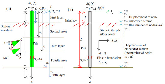
Figure 1.
Schematic diagram of the partially-embedded single pile in layered soil: (a) Laterally-loaded single pile; (b) Analytical model of pile–soil system.
The displacement components of the soil field around the partially-embedded single pile can ignore the vertical displacement. They can be written as:
where is the lateral displacement of the pile, is the vertical displacement components of the pile body displacement, and is the dimensionless function representing the variation of the soil displacement along the r direction.
Based on the assumption of displacements given in Equations (1)–(3) and the stress–strain relations, the potential energy of the pile and soil system is given by:
Correspondingly, the kinetic energy of the pile and soil system can be written as:
where and are the mass of the soil under the pile and the mass per linear meter of the pile, respectively, is the density of the soil around the pile.
The sum of work of non-conservative forces such as external force and bending moment can be written as:
Substituting Equations (4)–(6) into Hamilton’s principle formulation, we can obtain:
where
Therefore, the motion equation of the partially-embedded single pile can be obtained
where , , .
With boundary conditions:
Collecting the coefficients of for in Equation (7), we can obtain:
where
where .
The solution to Equation (13) is:
It is assumed that the pile is undergoing a steady-state harmonic motion. So let
Substituting Equations (16)–(18) into Equation (8) gives:
For free-fixed pile, boundary conditions at are:
For free-free pile, boundary conditions at are:
Solving the differential equation given in Equation (19), with the boundary conditions and , we get the following solution:
where
Meanwhile, the attenuation parameter can be written as:
2.2. Finite Difference Method
By ignoring the effect of external load and damping, Equation (19) can be rewritten as:
Taking free-free pile as an example, the boundary conditions are:
The discretization of Equations (34) and (35) using the FDM is performed as [18]
In Equations (39) and (40), the subscript in represents the displacements and , , of the non-embedded section and the embedded section of the pile and the subscript represents the number of nodes in this section and is the discretization expression of the mode shape function, which is derived using the Taylor series expansion [22].
In the range of , the second and fourth derivatives of can be written as:
Considering the virtual nodes and , from the boundary condition (36)–(38) we have
Substituting Equations (41)–(44) into Equation (40), we can obtain
In Equation (45), and are diagonal matrices and , where the subscript is the number of nodes in the non-embedded section, the subscript is the total number of nodes in a pile. Substituting Equations (36)–(38) into Equation (45), the matrix formulation of Equation (45) can be written as:
where , .
From Equations (36)–(38), we can obtain:
and so
where and are diagonal matrices and . In the same way, substituting boundary condition Equations (36)–(38) into Equation (49), the matrix formulation of Equation (49) can be obtained as:
where .
Considering the continuity condition in Equations (36)–(38), the diagonal matrix of the system is given by
where
Therefore, we can obtain the natural frequencies of each order of partially-embedded single piles by letting the matrix determinant Equation (51) be zero.
3. Green’s Functions for Dynamic Response
3.1. Embedded Section
We can assume that there is a simple harmonic lateral load at the pile top, which can be written as:
where is the Dirac function, is the frequency of the external excitation. We can let when calculating the Green’s functions for the dynamic response of the pile. For the pile top, .
Substitution of Equation (52) into Equation (35) gives:
where , , .
Using the Green’s function method, the solution of Equation (53) can be written as:
where is the function of the external excitation, is the Green’s function to be determined which is the solution of the following formulation:
From Equation (55), it is seen that . Laplace transformation is applied to the variable in Equation (55), we can obtain:
where , , , and are constants which can be determined by the boundary conditions. To obtain the inverse transform of , we assume that . We can get the results of the inverse transform by referring to the literature [23]:
where is the Heaviside function, and are functions specified by
From Equation (56), we can obtain:
Substitution of Equations (62)–(65) into Equation (66) gives the undetermined Green function
where are functions specified by
From Equations (62)–(65) and (68)–(72), we can obtain:
and so
Substitution of Equation (67) into Equation (54) gives the response function of the pile
Correspondingly, the dynamic response function of the embedded pile is given by
3.2. Non-Embedded Section
As described in Section 3.1, Equation (34) can be written as:
where .
Obviously, the solution of Equation (84) is given by
Applying the Laplace transform method for the variable in Equation (84), we can obtain:
where , , and are constants which can be determined by the boundary conditions of the pile.
To obtain the inverse transform of , we assume that .
From Equation (87), we can obtain:
where are functions specified by
Therefore, the response function of the non-embedded section of the pile is as follows:
The dynamic response function of the pile of the non-embedded section is given by
4. Numerical Calculations
4.1. Solution Process
According to the modified Vlasov foundation model, the lateral displacement of a partially-embedded single pile in a layered soil field can be obtained by iteratively solving attenuation parameters. The process is shown in Figure 2.
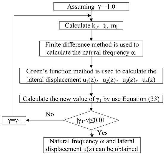
Figure 2.
Flow chart of calculation.
4.2. Validity of the Present Solutions
In order to verify the validity of the finite difference method, the calculation model of Prendergast et al. and the model and calculation method of this paper were used to solve the variation of the first-order natural frequencies of the steel pipe pile with a length of 8.76 m under scouring conditions. The results are compared with the results measured on-site [16].
As shown in Figure 3, when the pile (free-free pile or fixed-free pile) is analyzed under the scour conditions, the scour effect is considered by completely removing the entire soil layer to a certain depth. After scouring, part of the pile body is exposed to the soil surface, and the pile is treated as partially-embedded. In this paper, the pile is divided into 40 pile units. There is no pile–soil interaction above the scour depth so they can be regarded as beam elements. Moreover, they can be regarded as spring-beam elements because of the pile–soil interaction below the scour depth. In the process of numerical calculation, the initial pile’s length of the non-embedded section is 2.19 m (scour level is 0), which can be represented as 10 beam elements and 30 spring-beam elements. The scouring process is simulated by removing spring supports from top to bottom.
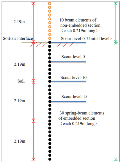
Figure 3.
Numerical model of the finite difference method and setting of scour levels.
The physical parameters of the pile and the foundation are shown in Table 1. The elastic modulus of the foundation is [18]:
where and are the soil’s density and Poisson’s ratio, respectively, and is the velocity of the compression wave (213 m/s for sand [18]).

Table 1.
Physical parameters of the single pile and foundation during the verification.
The subgrade reaction coefficient of the model of Prendergast et al. is [24]:
where is the outer diameter of the pile, and is the flexural rigidity of the pile.
Figure 4 shows the comparison of the first-order natural frequencies of the partially-embedded single pile under scouring obtained by the model of Prendergast et al., the method in this paper, and the actual measured dates on-site. Referring to Equation (97), the subgrade reaction force in the calculation model of Prendert et al. has nothing to do with the pile diameter. The first-order natural frequencies of the single pile obtained by Prendergast et al.’s calculation model have the same trend as the actual measured dates on-site. The first-order natural frequencies of the single pile calculated by the method in this paper are closer to the measured dates on-site, and they are highly consistent with the measured dates on-site within the range of common scour depth (1–3 m). The results of the calculation model in this paper can more effectively predict the dynamic characteristics of partially-embedded single piles under the scouring action.
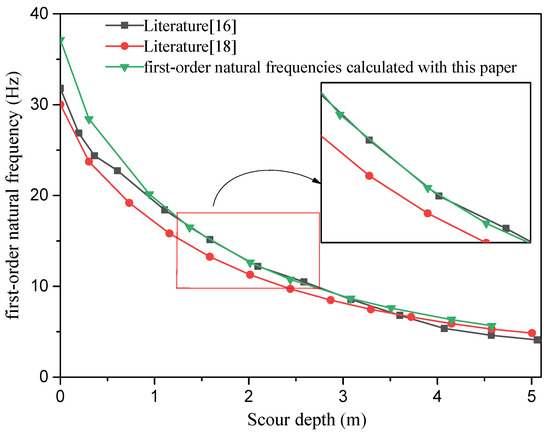
Figure 4.
Comparison of the first-order natural frequencies calculated by the finite difference method with the measurement result by Prendergast et al. [16,18].
The displacement curve of the single pile with pile diameter , slenderness ratio , dimensionless frequency is calculated by using the proposed model and the model presented by the literature [25], which assumes that the pile has a fixed end and a pile top with a constrained angle. The calculation results are compared with the results given by the literature [25] and demonstrated in Figure 5. It can be seen from Figure 5 that the calculation results in this paper are basically consistent with the literature [25], which verifies the validity of Green’s function method in this paper.
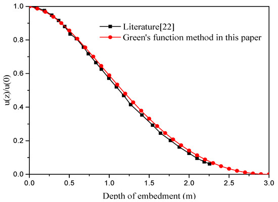
Figure 5.
Comparison of pile displacement calculated by Green’s functions method and the literature [22,25].
5. Parameter Analysis
5.1. Effect of Scour Depth
In this section, the effect of scour depth on the dynamic response of the partially-embedded single pile in layered soil is analyzed. Table 1 shows the physical parameters of the single pile and the layered soil required for the calculation. In the calculation, the partially-embedded single pile passes through the three-layer foundation. The geological condition from top to bottom is: the first layer is the loose sand layer (); the second layer is the medium sand layer (); the third layer is the tight sand layer (). For sand, the Poisson’s ratio is approximately 0.3. The lateral excitation amplitude of the pile top is . The setting of the scouring levels is shown in Figure 3, with each scouring level separated by 1.095 m.
Table 2 shows the variation of Vlasov foundation parameters and dynamic characteristics of partially-embedded single piles with the scour levels under the boundary conditions of free-free piles and fixed-free piles. Table 2 shows that the subgrade reaction coefficient of each layer of soil decreases with the increase in the scour levels, while the shear coefficient increases with the increase in the scour levels.
Table 2.
Effect of the scour on Vlasov foundation parameters and dynamic characteristics of the single pile.
The frequencies of each order of the partially-embedded single pile decrease rapidly with the increase in scouring levels. The depth of the embedded soil decreases with the scour process, and the pile–soil interaction effect gradually weakens.
The effect of the degree of scouring on the dynamic response amplitudes of the partially-embedded single pile in the layered soil fields is investigated in Figure 6. As shown in Figure 6, the displacement of the pile top of the single pile increases with the increase in the scour levels. When the scour level reaches 10, that is, the length of the non-embedded section of the pile satisfies ( is the pile length), the response amplitudes of the pile top of the partially-embedded single pile in the layered soil fields were greater than 0.01 m, and the single pile has presented lateral instability under dynamic load [26]. In addition, as the degree of scouring intensifies, the inverted point of the pile body moves downward, and the displacement at the inverted point increases gradually. The response amplitude of the free-free pile top is slightly larger than that of the free-fixed pile, and the difference between them increases with the increase in scour depth.
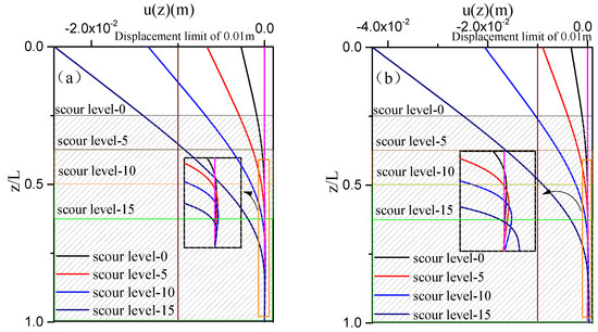
Figure 6.
Effect of the scour degree on the dynamic response of the single pile in layered foundation: (a) Free-fixed pile; (b) Free-free pile.
5.2. Effect of Soil Thickness
In the process of parameter analysis, the steel pipe piles in Table 1 are still used. The setting of the scouring levels is shown in Figure 3. Partially-embedded single piles pass through the three-layer foundation soil, the elastic modulus is 10, 20, 50 MPa from top to bottom, and the Poisson’s ratio is 0.3. In order to study the effect of the thickness of the bottom layer (third layer) of the layered soil fields on the dynamic response of a single pile, the depth of the first layer of soil is kept constant, and the thickness of the third layer is changed by changing the ratio of the thickness of the second and third layers of soil, in order: , , ; , , ; , , ( represents the thickness of the soil layer).
In order to more clearly explore the effect of the thickness of the underlying soil in the layered soil fields on the dynamic response of the partially-embedded single pile, Table 3 shows the effect of h3 on the first-order natural frequencies and amplitudes of the pile top of the pile under varied scour levels. It can be seen from Table 3 that the first-order natural frequencies of the single pile under each scour level increase with the increase in h3. In addition, as the scour degree intensifies, the natural frequencies decrease significantly, and the response amplitudes of the pile top increase significantly. When the scour level reaches 10, the lateral instability of a single pile appears.
Table 3.
Effect of the thickness of the underlying soil on dynamic characteristics of the single pile under varied scour levels.
The variations of the mode shapes of the partially-embedded single pile under varied scour levels with the change of the thickness of the underlying soil are investigated in Figure 7. It is shown that the response amplitudes of the pile top of the single pile and the displacement amplitudes at the inverted point of the pile body decrease with the increase in the thickness of the underlying soil, regardless of the degree of scour.
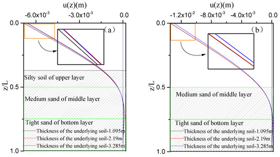
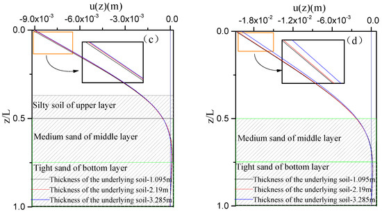
Figure 7.
Effect of the thickness of soil on the dynamic response of the single pile under varied scour levels: (a) Free-fixed pile, scour level-5; (b) Free-fixed pile, scour level-10; (c) Free-free pile, scour level-5; (d) Free-free pile, scour level-10.
5.3. Effect of Elastic Modulus of Soil
This section analyzes the effect of the elastic modulus of the first layer of soil on the dynamic characteristics of the partially-embedded single pile. The first layer of soil around the pile is: mucky soil layer (), loose sand layer (), silty sand layer () and medium sand layer (), successively. The second layer is the medium sand layer (). The third layer is the tight sand layer (). Table 4 shows the physical parameters of the single pile and layered soil field required for the calculation.
Table 4.
Physical parameters of the single pile and foundation in the parameter analysis.
Table 5 shows the variation of the first-order natural frequencies of the partially-embedded single pile and the response amplitudes of the pile top under varied scour levels with the elastic modulus of the first layer of soil. When the scour level is 10, the first layer of soil is completely cleared due to scour, so the dynamic characteristics of the single pile are the same. It can be seen from Table 5 that under each scour level, the response amplitudes of the pile top decrease significantly with the increase in the parameter , and the first-order natural frequencies of a single pile increase with the increase in the parameter . For example: if the elastic modulus of the soil increases by about 0.5 times, one time, and two times, the first-order natural frequencies of the single pile increase by about 10%, 20%, and 30%, respectively. The subgrade reaction coefficients of the elastic foundation increase with the increase in the elastic modulus of the soil, and accordingly, the lateral constraint of the soil field around the pile is strengthened.
Table 5.
Effect of the elastic modulus of soil on dynamic characteristics of the single pile under varied scour levels.
Figure 8 shows the variation of the mode shapes of the partially-embedded single pile under varied scour levels with the change of the elastic modulus of the first layer of soil. Overall, the effect of parameter on the mode shapes of the pile body is significant. With the increase in the parameter , the lateral displacement amplitudes of the pile top of the single pile under each scour level decrease, while the displacement amplitudes at the inverted point of the pile body increase referring to the detail drawn in Figure 8. Corresponding to the results shown in Table 5, with the increase in the elastic modulus of soil around the pile, the lateral constraint of soil around the pile on the pile foundation increases. The pile-soil interaction effect is enhanced and the lateral deformation of the partially-embedded single pile is reduced.
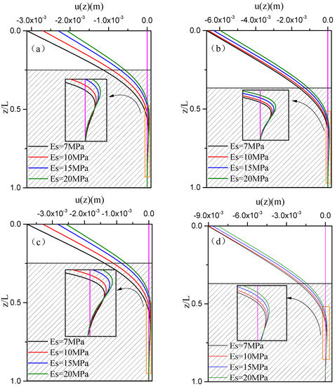
Figure 8.
Effect of the elastic modulus of soil on the dynamic response of the single pile under varied scour levels: (a) Free-fixed pile, scour level-0; (b) Free-fixed pile, scour level-5 (c) Free-free pile, scour level-0; (d) Free-free pile, scour level-5.
6. Conclusions
A dynamic model of the laterally-loaded single pile in layered soil is established employing Hamilton’s principle based on the modified Vlasov foundation model. The finite difference method and Green’s function method are combined to obtain the single pile’s first-order natural frequencies and dynamic response configuration. Then, numerical results and discussions are presented to explore the single pile’s dynamic characteristics and examine the effects of scouring, elastic modulus, and the thickness of layered soil on the dynamic response of the partially-embedded single pile in the layered soil fields. The conclusions are as follows:
- As the scour degree intensifies, the subgrade reaction coefficient of each layer of soil in the modified Vlasov foundation model decreases, and the shear coefficient increases. Furthermore, the first-order natural frequencies of the single pile in layered soil decrease significantly.
- When scouring to the length of the non-embedded section of the pile satisfies ( is the pile length), the partially-embedded single pile will demonstrate lateral instability under the action of dynamic load.
- As the thickness of the underlying soil increases, the first-order natural frequencies of the single pile under varied scour levels increase. During the response, amplitudes of the pile top decrease.
- As the elastic modulus of the first layer of soil increases, the first-order natural frequencies of the single pile increase, and the response amplitudes of the pile top decrease significantly, while the displacement amplitudes at the inverted point of the pile body increase. The elastic modulus of the first layer of soil is increased by about 0.5 times, 1 time and 2 times, and the first-order natural frequencies of the single pile increase by about 10%, 20%, and 30%.
The model in this paper has certain limitations, such as not considering the slip or separation phenomenon of the pile–soil interface and nonlinear dynamic analysis. The pile–soil dynamic response in most sites is particularly complex. As a weak part of the pile foundation, the pile–soil contact surface is prone to the damage of the soil around the pile and even the detachment of the contact surface, which leads to the lack of binding force of the soil and instability of the pile foundation. Therefore, in the future study of the dynamic response of pile foundations, it is necessary to explore the dynamic characteristics of the laterally-loaded piles, considering the weakening effect of the contact surface.
Author Contributions
Conceptualization, J.M.; methodology, J.M. and S.H.; software, S.H.; validation, S.H., X.G. and D.L.; formal analysis, J.M., Y.G. and Q.L.; investigation, X.G. and D.L.; resources, J.M.; data curation, S.H.; writing—original draft preparation, J.M. and S.H.; writing—review and editing, J.M., S.H. and Q.L.; funding acquisition, J.M. All authors have read and agreed to the published version of the manuscript.
Funding
This research was funded by the National Natural Science Foundation of China (grant number 11502072, 51878265 and 52178331), the Young-backbone Teacher Foundation of Colleges and Universities of Henan Province (grant number 2019GGJS076) and the Key R&D and Promotion Special Project in Henan Province—Science and Technology Research Project (grant number 212102310946).
Institutional Review Board Statement
Not applicable.
Informed Consent Statement
Not applicable. Written informed consent was obtained from the patients to publish this paper.
Data Availability Statement
Not applicable.
Acknowledgments
The authors greatly appreciate the comments from the reviewers, whose comments helped to improve the quality of the paper.
Conflicts of Interest
The authors declare no conflict of interest.
References
- Wang, L.H.; Liu, C.L.; Wang, L.J. A simplified method for assessing the dynamic behaviour of a pile in layered saturated soils that considers current scour. Comput. Geotech. 2020, 128, 103831. [Google Scholar] [CrossRef]
- Qi, W.G.; Gao, F.P.; Randolph, M.F.; Lehane, B.M. Scour effects on p–y curves for shallowly embedded piles in sand. Géotechnique 2016, 66, 648–660. [Google Scholar] [CrossRef]
- Liu, Y.J.; Liu, C. Effects of scour-hole dimensions on lateral behavior of piles in sands. Comput. Geotech. 2019, 111, 30–41. [Google Scholar]
- Lin, C.; Han, J.; Caroline, B.; Robert, L.P. Analysis of laterally loaded piles in sand considering scour hole dimensions. J. Geotech. Geoenvironmental Eng. 2014, 140, 04014024. [Google Scholar] [CrossRef]
- Zhang, H.; Chen, S.; Liang, F. Effects of scour-hole dimensions and soil stress history on the behavior of laterally loaded piles in soft clay under scour conditions. Comput. Geotech. 2017, 84, 198–209. [Google Scholar] [CrossRef]
- Ai, Z.Y.; Li, Z.X. Dynamic analysis of a laterally loaded pile in a transversely isotropic multilayered half-space. Eng. Anal. Bound. Elem. 2015, 54, 68–75. [Google Scholar] [CrossRef]
- Poulos, H.G. Single pile response to cyclic lateral load. J. Geotech. Eng. ASCE 1982, 108, 355–375. [Google Scholar] [CrossRef]
- Millán, M.; Domínguez, J. Simplified BEM/FEM model for dynamic analysis of structures on piles and pile groups in viscoelastic and poroelastic soil. Eng. Anal. Bound. Elem. 2009, 33, 25–34. [Google Scholar] [CrossRef]
- Novak, M. Dynamic stiffness and damping of piles. Can. Geotech. J. 1974, 11, 574–598. [Google Scholar] [CrossRef]
- Ma, J.J.; Liu, Q.J.; Zhao, Y.Y. Stability of beams on modified Vlasov foundation subjected to lateral loads acting on the ends. Chin. J. Geotech. Eng. 2008, 30, 850–854. [Google Scholar]
- Vallabhan, C.V.G.; Daloglu, A.T. Modified Vlasov model for beams on elastic foundations. J. Geotech. Geoenvironmental Eng. 1991, 117, 956–996. [Google Scholar] [CrossRef]
- Das, Y.C.; Sargand, S.M. Forced vibrations of laterally loaded piles. Int. J. Solids Struct. 1999, 36, 4975–4989. [Google Scholar] [CrossRef]
- Pise, P.J. Laterally loaded piles in a two-layer soil system. J. Geotech. Eng. Div. 1982, 108, 1177–1181. [Google Scholar] [CrossRef]
- Bash, D.; Salgado, R. Elastic analysis of laterally loaded pile in multi-layered soil. Geomech. Geoengin. Int. J. 2007, 2, 183–196. [Google Scholar] [CrossRef]
- Avaei, A.; Ghotbi, R.; Aryafar, M. Investigation of pile–soil interaction subjected to lateral loads in layered soils. Am. J. Eng. Appl. Sci. 2008, 1, 76–81. [Google Scholar] [CrossRef][Green Version]
- Prendergast, L.J.; Hester, D.; Gavin, K.; O’Sullivan, J.J. An investigation of the changes in the natural frequency of a pile affected by scour. J. Sound Vib. 2013, 332, 6685–6702. [Google Scholar] [CrossRef]
- Zucca, M.; Franchi, A.; Crespi, P.; Longrarini, N.; Ronca, P. The new foundation system for the transept reconstruction of the basilica di collemaggio. In Proceedings of the International Masonry Society Conferences, Milan, Italy, 9–11 July 2018; pp. 2441–2450. [Google Scholar]
- Bao, T.; Liu, Z. Evaluation of Winkler model and Pasternak model for dynamic soil-structure interaction analysis of structures partially embedded in soils. Int. J. Geomech. 2020, 20, 4019167. [Google Scholar] [CrossRef]
- Abu-hilal, M. Forced vibration of Euler–Bernoulli beams by means of dynamic Green functions. J. Sound Vib. 2003, 267, 191–207. [Google Scholar] [CrossRef]
- Foda, M.A.; Abduljabbar, Z. A dynamic Green function formulation for the response of a beam structure to a moving mass. J. Sound Vib. 1998, 210, 295–306. [Google Scholar] [CrossRef]
- Liang, F.; Zhang, H.; Huang, M. Influence of flood-induced scour on dynamic impedances of pile groups considering the stress history of undrained soft clay. Soil Dyn. Earthq. Eng. 2017, 96, 76–88. [Google Scholar] [CrossRef]
- LeVeque, R. Finite Difference Methods for Ordinary and Partial Differential Equations: Steady-State and Time-Dependent Problems; Society for Industrial and Applied Mathematics: Philadelphia, PA, USA, 2007; pp. 3–10. [Google Scholar]
- Asmar, N.H. Partial Differential Equations with Fourier Series and Boundary Value Problems; Dover Publications: New York, NY, USA, 2016; pp. 306–309. [Google Scholar]
- Ashford, S.A.; Juirnarongrit, T. Evaluation of pile diameter effect on initial modulus of subgrade reaction. J. Geotech. Geoenvironmental Eng. 2003, 129, 234–242. [Google Scholar] [CrossRef]
- Makris, N.; Gazetas, G. Dynamic pile-soil-pile interaction. Part II: Lateral and seismic response. Earthq. Eng. Struct. Dyn. 1992, 21, 145–162. [Google Scholar] [CrossRef]
- China Academy of Building Research. Technical Code for Building Pile Foundations: JGJ 94–2008, 1st ed.; China Construction Industry Press: Beijing, China, 2008; pp. 58–59. [Google Scholar]
Publisher’s Note: MDPI stays neutral with regard to jurisdictional claims in published maps and institutional affiliations. |
© 2022 by the authors. Licensee MDPI, Basel, Switzerland. This article is an open access article distributed under the terms and conditions of the Creative Commons Attribution (CC BY) license (https://creativecommons.org/licenses/by/4.0/).