Abstract
Skeleton-based human action recognition has attracted extensive attention due to the robustness of the human skeleton data in the field of computer vision. In recent years, there is a trend of using graph convolutional networks (GCNs) to model the human skeleton into a spatio-temporal graph to explore the internal connections of human joints that has achieved remarkable performance. However, the existing methods always ignore the remote dependency between joints, and fixed temporal convolution kernels will lead to inflexible temporal modeling. In this paper, we propose a multi-scale adaptive aggregate graph convolution network (MSAAGCN) for skeleton-based action recognition. First, we designed a multi-scale spatial GCN to aggregate the remote and multi-order semantic information of the skeleton data and comprehensively model the internal relations of the human body for feature learning. Then, the multi-scale temporal module adaptively selects convolution kernels of different temporal lengths to obtain a more flexible temporal map. Additionally, the attention mechanism is added to obtain more meaningful joint, frame and channel information in the skeleton sequence. Extensive experiments on three large-scale datasets (NTU RGB+D 60, NTU RGB+D 120 and Kinetics-Skeleton) demonstrate the superiority of our proposed MSAAGCN.
1. Introduction
With the development of Internet technology and the popularization of video acquisition equipment, video has become the main carrier of information. The amount of video data is exploding, and how to analyze and understand the content of videos becomes more and more important. As one of the important topics of video understanding, human action recognition has become the focus of research in the field of computer vision.
Action recognition learns the representation and motion information in the video by modeling the spatial and temporal information of the time sequence in the video, which can establish the mapping relationship between the video content and the action category and help a computer effectively be competent for the task of video understanding. Action recognition has extensive application prospects in motion analysis, intelligent monitoring, human-computer interaction, video information retrieval and so on.
In recent years, skeleton-based data has been used more and more widely in human motion recognition. The skeleton data is a compact representation of human motion information, usually composed of a series of time series of 3D coordinates of human body joints, which can significantly reduce the redundant information in calculations. Additionally, in complex scenes, compared with traditional RGB video or optical flow data, human skeleton data is more robust because it can ignore the interference of background information; therefore, the recognition performance will be better.
Earlier skeleton-based action recognition methods mainly used joint coordinates to form feature vectors by hand-designed approaches [1,2,3], and then aggregated these features for action recognition. However, it ignored the internal association of joint information, resulting in insufficient recognition accuracy.
In traditional deep learning methods, the skeleton sequence is usually fed into recurrent neural networks (RNN) or convolutional neural networks (CNN) for analysis, and its features are captured to predict action labels [4,5,6,7,8,9,10,11,12]. However, the representation of skeleton data as pseudo-images or coordinate vectors cannot well express the interdependence between the joints of the human body, which is particularly important for human body action recognition. In fact, it is more natural to regard human skeleton information as a graph, with human joints as nodes of the graph and human bones as edges. In recent years, with the development of graph convolutional networks, it has begun to be successfully applied to various scenarios.
Yan et al. [13] first used graph structure to model skeleton data and construct a series of spatio-temporal graph convolutions on the skeleton sequence to extract features for skeleton-based action recognition. Initially, the graph convolution is performed to make the joints capture the local structure information of its neighbor nodes. With the increase of GCN layers, the receptive field of joints will expand to capture a larger range of neighborhood information. In this way, the spatio-temporal GCN finally obtains the global structure information of the skeleton data.
However, there are some disadvantages in this method: 1. It only pays attention to the physical connection between joints but ignores the remote dependence of joints. There may also be potential connections between disconnected joints. For example, there is no direct connection between the hand and the head in the action of making a call, which is very important to recognizing the action. Ignoring the connection between these disconnected joints will have an impact on the performance of action recognition; 2. It uses a fixed 1D convolution to perform the temporal convolution operation. The receptive field of the temporal graph is predefined and not flexible enough, which will also affect the accuracy of action recognition; 3. A skeleton action sequence contains many frames, and each frame contains multiple joint points. For action recognition, we often only need to focus on the key frame and joint information, and too much redundant information will lead to a decrease in recognition performance.
In order to solve the above problems, we use the high-order polynomial of the skeleton adjacency matrix to perform graph convolution to realize the extraction of the long-distance dependence relationship between the joints and the multi-scale structural feature. The adjacency polynomial makes the distant neighbor joints reachable. We introduce high-order approximation to increase the receptive field of graph convolution and build a multi-scale adjacency matrix according to the hop distances between each joint and its neighbors, which can help to better explore the joints in the spatial feature information. For the modeling of the skeleton sequence in the temporal dimension, the temporal graph is composed of the corresponding joints in consecutive frames connected by the temporal edges. Existing methods [4,13,14,15,16] usually set a fixed temporal window length and use 1D convolution to complete the temporal convolution operation. Since the time window is predefined, it lacks flexibility when recognizing different actions. Thus, we propose a multi-scale temporal convolution module that contains three scales: long, medium and short, to obtain the time characteristics of different temporal domain receptive fields. Additionally, we introduce weights to adaptively adjust and dynamically combine the used temporal domain receptive fields, which can more effectively capture temporal features of the skeleton data.
With the rise of the attention mechanism [17,18,19,20], we can introduce attention modules into the network. From the spatial dimension, an action often only has close connections with a few joints. From the temporal dimension, an action sequence has a series of frames, each of which has a different importance for the final recognition accuracy. From the feature dimension, each channel also contains different semantic information. Therefore, we added spatial attention, temporal attention and channel attention modules to focus on key joints, frames and channels that have a great impact on action recognition.
We propose a novel architecture for skeleton-based action recognition; the basic structure in our proposed model is the spatio-temporal-attention module (STAM), which is composed of a multi-scale aggregate graph convolution network (MSAGCN) module, a multi-scale adaptive temporal convolution network (MSATCN) module and a spatio-temporal-channel attention (STCAtt) module, as shown in Figure 1. We propose a multi-scale GCN to construct a multi-order adjacency matrix to obtain the dependence of joints and their further neighbors in the spatial domain, thereby effectively extracting wider spatial information features. Then we propose a MSATCN containing three temporal convolution kernels to model temporal features in three different ranges of long, medium and short. We introduce the STCAtt module to focus on more meaningful frames and joints from the spatio-temporal and channel dimensions, respectively. Additionally, we have added residual links between the modules, which can effectively reuse the spatio-temporal and channel features, to capture the local and global features of the skeleton sequence. This network architecture can better model the spatial and temporal features of human actions for skeleton-based action recognition. In order to verify the effectiveness of our proposed GCN model, extensive experiments were performed on three large-scale datasets: NTU-RGBD, NTU-RGBD120 and Kinetics, and our model achieved great performance on these datasets.
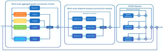
Figure 1.
The architecture of the proposed spatial-temporal-attention module (STAM). It contains a multi-scale aggregate graph convolution module for modeling spatial information of the skeleton sequence. Multi-scale adaptive temporal convolution module is used to capture temporal features of different time ranges (T1, T2 and T3), and the attention module is applied to focus on meaningful information. The residual connection is applied on each STAM. denotes element-wise sum, and denotes element-wise multiplication.
The main contributions of our work are as follows: (1) We propose a multi-scale aggregate GCN, which increases the connection between disconnected joints to better extract the spatial features of the skeleton data. (2) We design a TCN with a multi-scale convolution kernel to adaptively capture the temporal correlation of the skeleton sequence in different temporal length ranges and improve the generalization ability of the model. (3) We introduced an attention mechanism to focus on more meaningful joints, frames and channel features. (4) Extensive experiments have been performed on three public datasets: NTU-RGBD, NTU-RGBD120 and Kinetics, and our MSAAGCN has achieved very good performance.
2. Related Work
2.1. Skeleton-Based Action Recognition
In the task of human action recognition, skeleton data has received more and more attention due to its robustness and compactness. Traditional methods usually use hand-crafting [21,22,23] or learning [24,25] features of human joints to model the human body structure. However, these methods have the problem that the design process is too complicated, and they often ignore the internal relationship between the joints and cannot achieve satisfactory results. With the development of deep learning, CNN-based and RNN-based methods have gradually become the mainstream method for skeleton-based action recognition.
CNN-based methods [4,5,6,7,8] usually define a series of rules to formulate skeleton data into pseudo-images and feed them into the designed CNN network for action classification. RNN-based methods [9,10,11,12] usually model the skeleton sequence as a set of 2D or 3D joint coordinates, focusing on modeling the time dependence of the input sequence.
CNN-based methods: Li C et al. [26] proposed an end-to-end convolutional co-occurrence learning method, using CNN to learn co-occurrence features from skeleton data through a hierarchical aggregation method. Liang et al. [27] proposed a three-stream convolutional neural network method by fusing and learning three motion-related features (3D joints, joint displacements and oriented bone segments) to make full use of skeleton data, adding multi-task integrated learning to improve the generalization ability of the model. Zhang et al. [28] proposed a view adaptive method, which automatically adjusts the viewpoints of each frame to obtain the skeleton data representation under the new viewpoints, determines the appropriate viewpoint according to the input data and finally performs the action recognition through the main Long Short-Term Memory (LSTM) network.
RNN-based methods: Wang et al. [29] proposed a two-stream RNN architecture. In the temporal stream, it uses stacked RNN and hierarchical RNN to extract temporal features from joint coordinate sequences in different temporal ranges. In the spatial stream, the spatial graph of the skeleton is converted into the joint sequence, and then it inputs the sequence into the RNN to learn the spatial dependence of the joints. Li S et al. [30] proposed an independent recurrent neural network. The neurons in the same layer are independent of each other and are connected through cross-layers; it solves the common problems of gradient disappearance and explosion in traditional RNN and LSTM and can handle longer sequences and build a deeper network to learn the long-term dependencies in the skeleton sequence.
However, both CNN-based and RNN-based methods ignore the co-occurrence between spatial and temporal features in the skeleton sequence because the skeleton data is embedded in non-Euclidean geometric space, and these methods cannot handle non-Euclidean data well. In recent years, the graph convolutional network (GCN) has received more and more attention and is widely used in social networks and other fields. In fact, researchers find that it is more natural to describe skeleton data as a graph with human joints as nodes and bones as edges. GCN can effectively process non-European data and model-structured skeleton data. Yan et al. [13] first proposed a spatio-temporal graph convolution network to directly model the skeleton sequence into a graph structure and construct graph convolution to extract spatio-temporal features for action recognition, which achieved better performance than previous methods.
2.2. Graph Convolutional Network and Attention Mechanism
Graph convolutional network: Recently, GCN has been introduced to skeleton-based action recognition and has shown good performance. The principle of constructing GCNs on graphs is mainly divided into spatial methods [31,32] and spectral methods [33,34]. The spatial methods directly perform convolution operation on the graph node and its neighbor nodes to extract features based on the design rules. Additionally, the spectral methods use the eigenvalues and eigenvectors of the graph Laplacian to perform graph convolution in the frequency domain. Most of the existing GCN-based methods [13,15,16,35,36] focus on the design of graph topology.
Yan et al. [13] first proposed to utilize GCN to model the skeleton sequence. Shi et al. [15] proposed a two-stream adaptive graph convolutional network, which parameterizes the graph structure of the skeleton data, inputs it into the network and learns and updates features together with the model to increase the flexibility of GCN. Li M et al. [16] introduced the encoder–decoder structure to capture the implicit joint correlation between specific actions. It also expands the existing skeleton graph to express higher-order dependencies and combines actional and structural links to learn spatial and temporal features. Wen et al. [14] proposed a motif-based GCN, which models the dependency between physically connected and disconnected nodes to extract high-order spatial information and proposed a variable temporal dense block to capture temporal information in different ranges. Cheng et al. [37] proposed to use a lightweight shift operation to replace the 2D convolution operation, achieving excellent performance at a small computational cost. Ye et al. [35] introduced a lightweight and effective Context-encoding Network (CeN) to explore the context encoding information and added it to the GCN to automatically learn the skeleton topology. Peng et al. [36] applied the neural structure search and replaces the predefined graph structure with a dynamic graph structure to explore the generation mechanism of different graphs under different semantics.
Attention mechanism: The attention mechanism can help neural networks pay attention to the more important feature parts of the input information. Many researchers have added the attention mechanism to the action recognition tasks to better model the spatio-temporal graph structure. Liu et al. [17] focused on the joint information in the frame through the global context memory cell and introduced a recurrent attention mechanism, which solves the problem of the original LSTM network not having an explicit attention mechanism. Similarly, Zhang et al. [18] also proposed to add Element-wise-Attention Gate (EleAttG) to RNN, which enables RNN neurons to have the attention ability to adaptively modulate the input. Wen et al. [14] employed the non-local block to capture dependencies, which enhances the ability of the network to extract global temporal features. Xia et al. [38] proposed a spatial and temporal attention mask, which reuses important spatio-temporal features and enables GCN to aggregate global context information of the skeleton sequence.
3. Multi-Scale Adaptive Aggregate Graph Convolutional Network
The data of the human skeleton is usually obtained from video by multimodal sensors or a pose estimation algorithm. The skeleton data is a series of frames containing the corresponding joint coordinates. The 2D or 3D coordinate sequences of the joints are fed into the network, and we construct a spatio-temporal graph. The joints are regarded as nodes in the graph, and the bones connected by adjacent joints are regarded as edges in the graph. We design a multi-scale adaptive GCN, which can model the long-range spatial dependence of the human body structure and extract richer spatial action features. Then we concatenate the multi-order feature maps obtained by the spatial graph convolution operation and then feed them into temporal module, whose purpose is to process temporal information and learn the joint movement information in the temporal sequences to add temporal features for the graph. Additionally, the MSATCN we proposed can extract three forms of different temporal range feature information and aggregate them to obtain high-level feature maps. Moreover, we apply the STCAtt to enhance the representation of features.
3.1. Multi-Scale Aggregate Graph Convolution Module
For better action recognition based on skeleton graphs, multi-scale spatial structural features need to be paid attention to, while traditional methods only consider the physical connections between joints, ignoring that there are also potential correlations between disconnected joints in the structure. For example, there are multi-hop connections between the left hand and the right hand, but it is very important to recognize the action of clapping. Therefore, we propose a multi-scale aggregate graph convolution module to explore the relevance of human skeleton data in the same frame. As shown in Figure 2, we build the multi-order adjacency matrices and adopt an adaptive method in each adjacency matrix to learn the topological structure of the graph to improve the flexibility of modeling semantic information, and finally we aggregate the obtained multi-order information to explore the spatial feature information of the skeleton sequence.
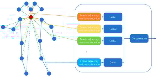
Figure 2.
Spatial graph of the skeleton (left) and multi-scale aggregate graph convolution module (right). In the graph, the solid nodes represent the body joints, and the edges represent the bones that connect the joints. The edges of different colors intuitively reflect the relationship between nodes with different hop connections.
In the graph convolutional network, we construct a graph to represent human skeleton data, where is the set of nodes that symbolizes the joints of the human body; is the set of edges of the skeleton connected by adjacent joints; and represents the adjacency matrix of the edge, which encodes the connection of the edge, that is, if the node and are connected, then ; otherwise, . We define , where represents the identity matrix, and is the adjacency matrix with self-connection. Since cannot be multiplied directly, we first need to standardize it. According to [39], the standardized Laplacian L can be formulated as , where the diagonal matrix , .
For the input , the graph convolution with filter can be expressed as ; represents the eigenvector matrix of ; is the Fourier transform of the graph of ; and can be regarded as a function of the eigenvector of . Hammond et al. [40] have mentioned that can be approximated by Chebyshev polynomials, which is formulated as
where , and represents the -order Chebyshev coefficient. Moreover, a Chebyshev polynomial is defined as , , .
According to [39], for the signal , it satisfies
means to calculate the difference between each vertex and its one-hop neighbor nodes. When , means the k-order connection, and means the difference between each vertex and its k-hop neighbor nodes, so it is possible to perform convolution operations on more neighbor nodes in a larger receptive field. Moreover, the spatial graph convolution with a receptive field of k can also be regarded as a linear transformation of the k-order Chebyshev polynomial. Finally, we define the spatial graph convolution operation as follows:
where is the weight matrix of , which can be learned by training in the network, and represents the bias; denotes the activation function.
We have observed that after each convolution operation in GCN, the network will aggregate the information of the joint and its neighbors connected via bones. This means that after multiple convolution operations, each node finally contains global information, but the early local information will be ignored. He et al. [41] proposed the concept of a residual link by introducing the residual structure, adding identity mapping to connect different layers of the network, and the input data information can be directly added to the output of the residual function. We consider adding residual links to reuse the local information of the node to obtain richer semantic information.
As shown in Figure 2, we define graph transformations of different orders according to the distance of hop connections between nodes, where 1-hop connection indicates a physical connection between nodes, and we aggregate multi-scale information through concatenate operations. The identity transformation is passed through the residual connection.
In order to improve the flexibility of the convolutional layer, inspired by the data-driven method from [15], we add the global graph and individual graph learned from the data to each order of the adjacency matrix and apply data-dependent and layer-dependent biases to the graph transformations of the matrix for more flexible connections so as to better learn the adaptive graph topology. Moreover, we add a graph mask, which is initialized to 1 and updated with the training process.
Feature aggregation: After the feature extraction of the adjacency matrix of each order is performed through the graph convolution transformation, the number of output features becomes 1/n, and then we aggregate them together through a concatenation layer, which consists of a batch normalization layer, a layer and a convolutional layer to maintain the original feature number.
3.2. Multi-Scale Adaptive Temporal Convolution Module
In the defined graph structure, the same joints between consecutive frames are connected by temporal edges (green lines in Figure 1). We choose to decompose the spatio-temporal graph into two spatial and temporal sub-modules instead of directly performing graph convolution operations on the spatio-temporal graph. This is because the strategy of the spatio-temporal decomposition method is easier to learn [14]. For the graph of frame t, we first feed it into the spatial graph convolution and then concatenate its output information with the time axis to obtain a 3D tensor, which is fed into the temporal module for action recognition.
For temporal convolution, current methods [13] usually use 1D convolution to obtain temporal features. Since the convolution kernel size is fixed to , it is often difficult to flexibly capture some temporal correlations of the skeleton data. Moreover, different action classes in the dataset may require different temporal receptive fields. For example, there are actions that can be judged within a short time range, such as falling down, and actions that can be judged within a longer time range, such as carrying a plate. Therefore, we designed a multi-scale temporal convolution module to adaptively extract the feature correlations on the temporal sequence. We use three convolution kernels with kernel sizes of , and to model the features in three different temporal scales of short, middle and long terms, respectively, and add the weight coefficients to adaptively adjust the scales of different importance. The proposed multi-scale temporal convolution operation can be formulated as
where denotes the concatenate operation. denotes the weight, which is used to adjust the importance of time features at different scales. Through the dynamic adjustment of the weight, the model can adaptively extract temporal features in different scales to improve the generalization ability of the temporal convolution module.
3.3. Spatial-Temporal-Channel Attention Module
The attention mechanism is a resource allocation mechanism, which redistributes the originally evenly allocated resources according to the importance of the focus. Inspired by [42,43], here we propose an attention mechanism, which contains three modules of spatial attention, temporal attention and channel attention mask.
Spatial attention module: In the spatial dimension, the movement range and dynamics of each joint in different actions are different. We can use the attention mechanism to help the model adaptively capture the dynamic correlation of each joint in the spatial dimension based on different levels of attention. By using the spatial relationship of features to generate the spatial attention mask , average pooling can learn from the target object and calculate spatial statistics [19,44], and maximum pooling can extract another important clue of object features to infer more refined attention. Using both types of pooling can improve the network representation ability [42]. It is formulated as
where is the input feature map, represent the number of channels, frames and joints, respectively; and represent the average-pooling and max-pooling operation; represents the connection operation; represents the 2D convolution operation; and represents the activation function. , as shown in the attention module in Figure 1; we calculate the product of the attention map and the input feature map, and then the input is connected with the result to refine.
where denotes element-wise multiplication.
Temporal attention module: In the time dimension, there is a correlation between the joint points of different frames, and the correlation between frames of different actions is also different. Similarly, we can use the attention mechanism to adaptively give them different weights. It is formulated as
where , and other symbols are similar to the spatial attention module.
Channel attention module: according to [19], each layer of the convolutional network has multiple convolution kernels, and each convolution kernel corresponds to a feature channel. The channel attention mechanism allocates resources between each convolution channel. We first perform feature compression through the squeeze operation, use global average-pooling to generate the statistics of each channel and then utilize the excitation operation to explicitly model the correlation between the feature channels through parameters and generate weights representing importance for each feature channel. Finally, we reweight the feature map, which is weighted to the previous feature channel by channel through multiplication. Similarly, we can formulate it as
where and are learnable weights; is used for dimensionality reduction; is used to calculate attention weights; and represents the activation function.
3.4. Multi-Stream Framework
The skeleton-based action recognition methods usually utilize the coordinate in the joint information of the input skeleton sequence. Shi et al. [15] found that the bone information connected by the joints is also very helpful for the action recognition and proposed a two-stream framework using joint and bone information. Moreover, the motion information of the joints has a potential effect on action recognition. For example, standing up and sitting down have no difference only from the joint coordinates and bone information, but it is easy to recognize by adding the motion information. In our work, the input data is mainly divided into node information, bone information and motion information.
First, we define the original 3D coordinate set of a skeleton sequence as , where represents the joint coordinates, and and denote the numbers of frames and joints, respectively.
We suppose that the joint feature set is , where represents the coordinates of the v-th joint in the t-th frame. Additionally, the relative coordinate set is , where , and denotes the center joint of the skeleton sequence. We concatenated these two sets into a sequence as the input of the joint information stream.
Then we calculate the bone and the motion information based on the joint information. Additionally, these two information streams expand the matrix by filling in 0 elements to compensate for the change in dimensionality. Suppose that the bone length information set is , where denotes the neighbors of joint . The bone length angle set is , and the angle can be calculated by
where represents the joint coordinates. We concatenate these two sets into a sequence as the input of the bone information stream.
Additionally, we suppose that the motion velocity information set , where , and the motion velocity difference information set is , where . We concatenate these two sets into a sequence as the input of the motion information stream.
We separately input the joints, bones and motion data into our network, and we add the scores of these streams to obtain the final classification result.
3.5. Network Architecture
As shown in Figure 3, the main architecture of our network is a stack of 9 basic modules named STAM (as shown in Figure 1), which contains MSAGCN, MSATCN and STCAtt blocks. Additionally, we introduced residual links to connect each module and each block in the module to capture more abundant context information. First, the original skeleton data passes through the batch normalization (BN) layer for data normalization, and then the normalized data is input into the MSAGCN block. The input and output channels of these modules are (6, 64), (64, 64), (64, 64), (64, 128), (128, 128), (128, 128), (128, 256), (256, 256) and (256, 256). The features extracted from the last module are sent to the global average-pooling layer, and then the classifier is used to obtain the final classification result.
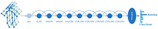
Figure 3.
The overall architecture of our multi-scale adaptive aggregate graph convolutional network. It consists of 9 basic modules (as shown in Figure 1), which are indicated by dark-colored circles, and the numbers below these circles indicate their input and output channels, respectively. Each module contains the residual links in the figure. Light-colored BN circle represents batch normalization layer for data normalization, and the standard Softmax classifier is used for action category.
4. Experiments
4.1. Datasets
NTU-RGB-D 60: NTU-RGB-D [45] is currently the most widely used action recognition dataset. It consists of 56,880 video clips in a total of 60 classes of actions performed by 40 subjects aged 10 to 35 years old. Each video clip contains an action, and each clip has 4 modalities: RGB video, depth map sequence, 3D skeleton data and infrared video. The data is captured by three Microsoft Kinect v.2 cameras at the same time, and the cameras are set at three different horizontal angles: , and . We used the 3D skeleton data in the experiment, which was obtained through the skeleton tracking technology in the Kinect camera. It is composed of the 3D position coordinates of the 25 main body joints of the human body, and there are at most two people in each clip sample. Two benchmarks are recommended in the dataset: cross-subject (X-sub) and cross-view (X-view). (1) For the cross-subject setting, the data is divided into training set and validation set, which contain 40320 video clips and 16,560 video clips, respectively. The subjects in the two sets are different, and 40 subjects are divided into a training group and a test group, each group containing 20 subjects. (2) For the cross-view setting, we select 18960 video clips captured by camera view 1 at for testing, 37,920 clips captured by camera views 2 and 3 at and for training. There are 302 video samples that need to be ignored. Following the convention in [45], we report the Top-1 accuracy on both benchmarks to evaluate recognition performance.
NTU-RGB-D 120: NTU-RGB+D 120 [46] is an extended version of the NTU-RGB+D dataset. It consists of 114480 video clips in a total of 120 classes of actions performed by 106 distinct subjects from 15 different countries, and each subject has a consistent ID number. The author of the dataset recommends two benchmarks: cross-subject(X-sub) and cross-setup(X-setup). (1) For the cross-subject setting, 106 subjects are divided into training group and testing group (including 63,026 and 50,922 clips respectively), half of which are used for training and the other half are used for testing. (2) For the cross-setup setting, the training data comes from 54,471 video clips with even setup ID numbers, and the testing data comes from 59,477 clips with the remaining odd setup ID numbers. Among them, 532 bad video samples should be ignored. Following the convention in [46], we report the Top-1 accuracy on both benchmarks.
Kinetics: Kinetics [47] is a large-scale video dataset for human action recognition, which contains about 300,000 video clips collected from YouTube; each clip is about 10 s. There are 400 action classes in the dataset, and there are at least 400 videos for each action. Since Kinetics only contains the original video clips, Yan et al. [13] used the OpenPose toolbox to extract the skeleton data of the original data and estimated the position of each person’s 18 joints on each frame. The tool can generate 2D coordinates and confidence scores from the video clip, and we use to represent the joint. We selected the two people with the highest joint confidence if a clip contained multiple people. The dataset provides 240,000 clips as the training set and 20,000 clips as the validation set. We trained the model on the training set, and we used the Top-1 accuracy rate and Top-5 accuracy rate to evaluate the model on the validation set. Following the convention in [47], we used two metrics: (1) Top-1 accuracy and (2) Top-5 accuracy to evaluate the validation set.
4.2. Implementation Details
In the experiment, the deep learning framework we used was PyTorch. In order to save computing resources and improve computing efficiency, we chose SGD with a Nesterov momentum of 0.9 and weight decay of 0.0001 to optimize the model, and cross-entropy loss was used as the loss function. In the MSATCN, we set the kernel size . All our models were trained on two NVIDIA Tesla V100 GPUs.
For the NTU-RGB+D and NTU-RGB+D 120 datasets, each sample contained at most two people. If the number of people was less than 2, then we filled it with 0. We set the fixed number of frames in each sample to 300 frames. For samples less than 300 frames, we fill themed up to 300 frames by repeating the samples. For these two datasets, we set the batch size to 64, and the maximum numbers of training epochs were set to 50 and 60, respectively. The learning rate was initialized to 0.1 and multiplied by 0.1 at epochs 30 and 40 for NTU RGB+D and at epochs 30 and 50 for NTU RGB+D 120. Additionally, in the first 5 epochs, we used the warmup strategy [41] to ensure the stability of training process.
For the Kinetics dataset, we used the data processing method in [13]; the batch size was set to 128, and the training epoch was set to 70. The learning rate was initialized to 0.1 and was multiplied by 0.1 at epochs 40, 50 and 60.
4.3. Ablation Study
In this section, we examined the effectiveness of our proposed components in MSAAGCN through experiments, and we used the recognition accuracy as an evaluation metric.
4.3.1. MSAAGCN
We first added adjacency matrices of different orders and observed the changes in the recognition accuracy of the model to prove the effectiveness of our proposed multi-scale adaptive aggregate GCN. Since the maximum distance between the two joints in the NTU-RGB-D dataset was 12, we chose the maximum number of scales N to be 12. As shown in Table 1, we have verified the recognition accuracy of the model after aggregation of 1, 2, 4, 8 and 12-order adjacency matrices on the NTU-RGB-D X-sub dataset. Obviously, the more adjacency matrices are aggregated, the better the recognition accuracy, which shows that each adjacency matrix is useful for model performance. However, when we aggregate to higher-order matrices, the performance improvement of the model becomes smaller. This may be due to the small dependence of the recognition of most actions on the distant joints. We used N = 12 for MSAGCN to conduct the following experiment.

Table 1.
Recognition accuracy (%) with different scale aggregation on X-sub benchmarks of the NTU RGB+D dataset.
In order to verify the effectiveness of the various modules in our proposed spatio-temporal network, including MSAGCN, MSATCN and STCAtt modules, we conducted experiments on a NTU-RGB-D X-sub benchmark to show the performance of the model with and without these modules. As shown in Table 2, we used Js-AGCN (Joint stream from 2s-AGCN [15]) as the baseline for comparison experiments. In order to ensure the fairness of the experiment, we first used the original spatial convolution and temporal convolution modules in Js-AGCN to test the recognition accuracy of the network model. Then we replaced the original spatial convolution module with the MSAGCN modules, and we found that the accuracy of the model improved 1.1%. This shows that the multi-scale aggregate graph convolution operation can extract more features from the input skeleton sequence, which is helpful for better classification. Next, we used the MSATCN module with kernel size to replace the original temporal convolution module, which improves the accuracy of the model by 0.6%. This shows that the use of a fixed temporal convolution kernel will make the temporal features indistinct, and the multi-scale temporal convolution can effectively capture the features of different temporal ranges. Finally, we used both the MSAGCN and MSATCN modules to replace the original modules, and the accuracy of the model increased to 87.8%, which shows that our proposed MSAGCN and MSATCN can more effectively capture the spatio-temporal features of the skeleton data.
Table 2.
Recognition accuracy with different combination of MSAGCN and MSATCN on the NTU RGB+D X-sub benchmarks.
4.3.2. Attention Mechanism
To verify the advantages of the STCAtt module we proposed in Section 3.3, we first separately tested the recognition accuracy of adding the spatial attention module, the temporal attention module and the channel attention module, respectively. Then we evaluated the performance of the model that concatenates the three modules sequentially. As shown in Table 3, the results indicate that the model with STCAtt achieves the best performance on NTU-RGB-D X-sub and NTU-RGB-D 120 X-sub120 benchmarks. We noticed that the model accuracy is not significantly improved (+0.5%) on the X-sub benchmark, while there is an obvious improvement (+1.9%) on the X-sub120 benchmark. We think this is because the accuracy on the X- sub benchmark is already high enough, and STCAtt is more robust to complex datasets such as NTU-RGB-D 120.
Table 3.
Comparisons of the recognition accuracy with different attentions on the X-sub and X-sub120 benchmarks.
4.3.3. Multi-Stream Framework
Here we verify the effectiveness of the multi-stream framework proposed in Section 3.4. As shown in Table 4, we test the performance of the model when inputting three different data streams of joint, bone and motion. Additionally, we obtain the results by inputting different combinations of these streams. Obviously, the model combining the three streams achieves the best recognition accuracy, and each stream contributes to the improvement of model performance.
Table 4.
Comparisons of the recognition accuracy with a different input stream on the NTU RGB+D X-sub benchmark.
4.4. Comparison with State-of-the-Art Methods
We compared our final model with state-of-the-art skeleton-based action recognition methods on the three datasets of NTU-RGB-D 60, NTU-RGB-D 120 and Kinetics. These methods for comparison include RNN-based methods [7,11,17], CNN-based methods [26,28,45,48] and GCN-based methods [13,14,15,16,36,37,49,50,51,52,53,54,55].
In the NTU-RGB-D 60 and NTU-RGB-D 120 datasets, we obtained the top-1 recognition accuracies on the two recommended benchmarks (X-sub, X-view) and (X-sub120, X-set120), which are shown in Table 5 and Table 6, respectively. Additionally, in the Kinetics dataset, the human joints data was obtained by an OpenPose toolbox, which is not as standardized as in NTU-RGB-D dataset, which can help verify the effectiveness of the model when the data is inaccurate. The recognition task is more challenging due to the variety of actions; we report the top-1 and top-5 recognition accuracies, as shown in Table 7. Our model achieved great results on both of the datasets, which verifies the superiority of our proposed model.
Table 5.
Comparisons of the Top-1 recognition accuracy with the state-of-the-art methods on the NTU RGB+D dataset.
Table 6.
Comparisons of the Top-1 recognition accuracy with the state-of-the-art methods on the NTU RGB+D120 dataset.
Table 7.
Comparisons of the Top-1 and Top-5 recognition accuracy with the state-of-the-art methods on the Skeleton-Kinetics dataset.
4.5. Discussion
Our method achieves good performance, but there are still some actions that are difficult to recognize. Figure 4 shows the recognition accuracy of our method on the NTU RGB+D X-Sub dataset. We have observed that there are three actions with a relatively low accuracy (less than 70%), which are reading, writing and playing with a phone. Figure 5 presents the five key frames of the actions writing and playing with a phone. It is easy to find that both of the actions are performed by two hands, and they are very similar. Moreover, the hands are abstracted into two joints in the dataset, which causes difficulty in recognition. How to accurately model the finer correlations between the joints to better recognize these actions is the next problem we plan to solve.
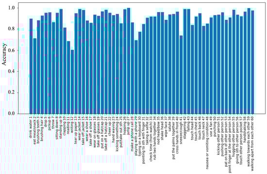
Figure 4.
The recognition accuracy of 60 action classes on NTU RGB+D X-Sub.
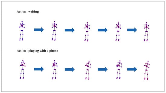
Figure 5.
Visualization of the two actions of writing and playing with a phone. For each action, we selected five key frames to represent.
5. Conclusions
In this work, we proposed a multi-stream model consisting of multi-scale aggregate GCN, multi-scale adaptive TCN and STCAtt modules for skeleton-based action recognition. We fed the skeleton sequence into the spatio-temporal module and constructed multi-order adjacency matrices in the spatial module to obtain the remote dependence and multi-scale semantic information of the joints. In the temporal module, we added a temporal convolution kernel with three ranges of long, medium and short to provide a more flexible receptive field for the temporal feature map. Additionally, we introduced an attention mechanism to focus on distinct key joints and frames and channel information to avoid the interference of redundant information. Moreover, we improved the utilization of features through residual connections between blocks and modules. Finally, with extensive ablation experiments and comparison experiments on three large-scale datasets, the results show that our proposed model achieves good performance.
Author Contributions
Conceptualization, Z.Z. and Y.W.; methodology, Y.W.; software, Y.W.; validation, Z.Z. and J.W.; formal analysis, Z.Z.; investigation, X.Z.; resources, Z.Z.; data curation, J.W.; writing—original draft preparation, Y.W.; writing—review and editing, Y.W.; visualization, X.Z.; supervision, X.Z.; project administration, J.W.; funding acquisition, Z.Z. All authors have read and agreed to the published version of the manuscript.
Funding
This research was funded by [the National Key Research and Development Program] grant number [2018YFCO824401] and [the National Natural Science Foundation of China] grant number [61872324].
Data Availability Statement
Publicly available datasets were analyzed in this study. NTU RGB+D and NTU-RGB-D 120: https://rose1.ntu.edu.sg/dataset/actionRecognition/ (accessed on 26 December 2021). Kinetics-Skeleton: https://github.com/yysijie/st-gcn/blob/master/OLD_README.md (accessed on 26 December 2021).
Conflicts of Interest
The authors declare no conflict of interest.
References
- Cai, Q.; Deng, Y.; Li, H. Survey on Human Action Recognition Based on Deep Learning. Comput. Sci. 2020, 47, 85–93. [Google Scholar]
- Yang, X.; Tian, Y.L. Eigenjoints-based action recognition using naive-bayes-nearest-neighbor. In Proceedings of the 2012 IEEE Computer Society Conference on Computer Vision and Pattern Recognition Workshops, Providence, RI, USA, 16–21 June 2012; IEEE: Piscataway, NJ, USA, 2012; pp. 14–19. [Google Scholar]
- Yang, X.; Tian, Y.L. Effective 3d action recognition using eigenjoints. J. Vis. Commun. Image Represent. 2014, 25, 2–11. [Google Scholar] [CrossRef]
- Li, B.; Dai, Y.; Cheng, X.; Chen, H.; Lin, Y.; He, M. Skeleton based action recognition using translation-scale invariant image mapping and multi-scale deep CNN. In Proceedings of the 2017 IEEE International Conference on Multimedia & Expo Workshops (ICMEW), Hong Kong, China, 10–14 July 2017; IEEE: Piscataway, NJ, USA, 2017; pp. 601–604. [Google Scholar]
- Li, C.; Zhong, Q.; Xie, D.; Pu, S. Skeleton-based action recognition with convolutional neural networks. In Proceedings of the 2017 IEEE International Conference on Multimedia & Expo Workshops (ICMEW), Hong Kong, China, 10–14 July 2017; IEEE: Piscataway, NJ, USA, 2017; pp. 597–600. [Google Scholar]
- Liu, H.; Tu, J.; Liu, M. Two-stream 3d convolutional neural network for skeleton-based action recognition. arXiv 2017, arXiv:1705.08106. [Google Scholar]
- Liu, M.; Liu, H.; Chen, C. Enhanced skeleton visualization for view invariant human action recognition. Pattern Recognit. 2017, 68, 346–362. [Google Scholar] [CrossRef]
- Cao, C.; Lan, C.; Zhang, Y.; Zeng, W.; Lu, H.; Zhang, Y. Skeleton-based action recognition with gated convolutional neural networks. IEEE Trans. Circuits Syst. Video Technol. 2018, 29, 3247–3257. [Google Scholar] [CrossRef]
- Du, Y.; Wang, W.; Wang, L. Hierarchical recurrent neural network for skeleton based action recognition. In Proceedings of the IEEE Conference on Computer Vision and Pattern Recognition, Boston, MA, USA, 7–12 June 2015; pp. 1110–1118. [Google Scholar]
- Zheng, W.; Li, L.; Zhang, Z.; Huang, Y.; Wang, L. Relational network for skeleton-based action recognition. In Proceedings of the 2019 IEEE International Conference on Multimedia and Expo (ICME), Shanghai, China, 8–12 July 2019; IEEE: Piscataway, NJ, USA, 2019; pp. 826–831. [Google Scholar]
- Liu, J.; Shahroudy, A.; Xu, D.; Wang, G. Spatio-temporal lstm with trust gates for 3D human action recognition. In European Conference on Computer Vision; Springer: Cham, Switzerland, 2016; pp. 816–833. [Google Scholar]
- Song, S.; Lan, C.; Xing, J.; Zeng, W.; Liu, J. An end-to-end spatio-temporal attention model for human action recognition from skeleton data. In Proceedings of the AAAI Conference on Artificial Intelligence, San Francisco, CA, USA, 4–9 February 2017; p. 31. [Google Scholar]
- Yan, S.; Xiong, Y.; Lin, D. Spatial temporal graph convolutional networks for skeleton-based action recognition. In Proceedings of the 32nd AAAI Conference on Artificial Intelligence, New Orleans, LA, USA, 2–7 February 2018. [Google Scholar]
- Wen, Y.H.; Gao, L.; Fu, H.; Zhang, F.L.; Xia, S. Graph CNNs with motif and variable temporal block for skeleton-based action recognition. In Proceedings of the AAAI Conference on Artificial Intelligence, Honolulu, HI, USA, 27 January–1 February 2019; Volume 33, pp. 8989–8996. [Google Scholar]
- Shi, L.; Zhang, Y.; Cheng, J.; Lu, H. Two-stream adaptive graph convolutional networks for skeleton-based action recognition. In Proceedings of the IEEE/CVF Conference on Computer Vision and Pattern Recognition, Long Beach, CA, USA, 15–20 June 2019; pp. 12026–12035. [Google Scholar]
- Li, M.; Chen, S.; Chen, X.; Zhang, Y.; Wang, Y.; Tian, Q. Actional-structural graph convolutional networks for skeleton-based action recognition. In Proceedings of the IEEE/CVF Conference on Computer Vision and Pattern Recognition, Long Beach, CA, USA, 15–20 June 2019; pp. 3595–3603. [Google Scholar]
- Liu, J.; Wang, G.; Duan, L.Y.; Abdiyeva, K.; Kot, A.C. Skeleton-based human action recognition with global context-aware attention LSTM networks. Proc. IEEE Trans. Image Processing 2017, 27, 1586–1599. [Google Scholar] [CrossRef] [PubMed] [Green Version]
- Zhang, P.; Xue, J.; Lan, C.; Zeng, W.; Gao, Z.; Zheng, N. Adding attentiveness to the neurons in recurrent neural networks. In Proceedings of the European Conference on Computer Vision (ECCV), Munich, Germany, 8–14 September 2018; pp. 135–151. [Google Scholar]
- Hu, J.; Shen, L.; Sun, G. Squeeze-and-excitation networks. In Proceedings of the IEEE Conference on Computer Vision and Pattern Recognition, Salt Lake City, UT, USA, 18–23 June 2018; pp. 7132–7141. [Google Scholar]
- Wang, F.; Jiang, M.; Qian, C.; Yang, S.; Li, C.; Zhang, H.; Wang, X.; Tang, X. Residual attention network for image classification. In Proceedings of the IEEE Conference on Computer Vision and Pattern Recognition, Honolulu, HI, USA, 21–26 July 2017; pp. 3156–3164. [Google Scholar]
- Hussein, M.E.; Torki, M.; Gowayyed, M.A.; El-Saban, M. Human action recognition using a temporal hierarchy of covariance descriptors on 3d joint locations. In Proceedings of the 23rd International Joint Conference on Artificial Intelligence, Beijing, China, 3–9 August 2013. [Google Scholar]
- Vemulapalli, R.; Arrate, F.; Chellappa, R. Human action recognition by representing 3D skeletons as points in a lie group. In Proceedings of the IEEE Conference on Computer Vision and Pattern Recognition, Columbus, OH, USA, 23–28 June 2014; pp. 588–595. [Google Scholar]
- Weng, J.; Weng, C.; Yuan, J. Spatio-temporal naive-bayes nearest-neighbor (st-nbnn) for skeleton-based action recognition. In Proceedings of the IEEE Conference on Computer Vision and Pattern Recognition, Honolulu, HI, USA, 21–26 July 2017; pp. 4171–4180. [Google Scholar]
- Xu, K.; Hu, W.; Leskovec, J.; Jegelka, S. How powerful are graph neural networks? arXiv 2018, arXiv:1810.00826. [Google Scholar]
- Ying, R.; You, J.; Morris, C.; Ren, X.; Hamilton, W.L.; Leskovec, J. Hierarchical graph representation learning with differentiable pooling. arXiv 2018, arXiv:1806.08804. [Google Scholar]
- Li, C.; Zhong, Q.; Xie, D.; Pu, S. Co-occurrence feature learning from skeleton data for action recognition and detection with hierarchical aggregation. arXiv 2018, arXiv:1804.06055. [Google Scholar]
- Liang, D.; Fan, G.; Lin, G.; Chen, W.; Pan, X.; Zhu, H. Three-stream convolutional neural network with multi-task and ensemble learning for 3d action recognition. In Proceedings of the IEEE/CVF Conference on Computer Vision and Pattern Recognition Workshops, Long Beach, CA, USA, 16–17 June 2019. [Google Scholar]
- Zhang, P.; Lan, C.; Xing, J.; Zeng, W.; Xue, J.; Zheng, N. View adaptive neural networks for high performance skeleton-based human action recognition. IEEE Trans. Pattern Anal. Mach. Intell. 2019, 41, 1963–1978. [Google Scholar] [CrossRef] [PubMed] [Green Version]
- Wang, H.; Wang, L. Modeling temporal dynamics and spatial configurations of actions using two-stream recurrent neural networks. In Proceedings of the IEEE Conference on Computer Vision and Pattern Recognition, Honolulu, HI, USA, 21–26 July 2017; pp. 499–508. [Google Scholar]
- Li, S.; Li, W.; Cook, C.; Gao, Y. Deep independently recurrent neural network (indrnn). arXiv 2019, preprint. arXiv:1910.06251. [Google Scholar]
- Niepert, M.; Ahmed, M.; Kutzkov, K. Learning convolutional neural networks for graphs. In Proceedings of the International Conference on Machine Learning, PMLR, New York, NY, USA, 20–22 June 2016; pp. 2014–2023. [Google Scholar]
- Monti, F.; Boscaini, D.; Masci, J.; Rodola, E.; Svoboda, J.; Bronstein, M.M. Geometric deep learning on graphs and manifolds using mixture model cnns. In Proceedings of the IEEE Conference on Computer Vision and Pattern Recognition, Honolulu, HI, USA, 21–26 July 2017; pp. 5115–5124. [Google Scholar]
- Defferrard, M.; Bresson, X.; Vandergheynst, P. Convolutional neural networks on graphs with fast localized spectral filtering. Adv. Neural Inf. Processing Syst. 2016, 29, 3844–3852. [Google Scholar]
- Henaff, M.; Bruna, J.; LeCun, Y. Deep convolutional networks on graph-structured data. arXiv 2015, arXiv:1506.05163. [Google Scholar]
- Ye, F.; Pu, S.; Zhong, Q.; Li, C.; Xie, D.; Tang, H. Dynamic GCN: Context-enriched Topology Learning for Skeleton-based Action Recognition. In Proceedings of the 28th ACM International Conference on Multimedia, Seattle, WA, USA, 2–16 October 2020; pp. 55–63. [Google Scholar]
- Peng, W.; Hong, X.; Chen, H.; Zhao, G. Learning graph convolutional network for skeleton-based human action recognition by neural searching. In Proceedings of the AAAI Conference on Artificial Intelligence, Hilton New York Midtown, NY, USA, 7–12 February 2020; Volume 34, pp. 2669–2676. [Google Scholar]
- Cheng, K.; Zhang, Y.; He, X.; Chen, W.; Cheng, J.; Lu, H. Skeleton-based action recognition with shift graph convolutional network. In Proceedings of the IEEE/CVF Conference on Computer Vision and Pattern Recognition, Seattle, WA, USA, 13–19 June 2020; pp. 183–192. [Google Scholar]
- Xia, H.; Gao, X. Multi-scale mixed dense graph convolution network for skeleton-based action recognition. IEEE Access 2021, 9, 36475–36484. [Google Scholar] [CrossRef]
- Gao, X.; Hu, W.; Tang, J.; Liu, J.; Guo, Z. Optimized skeleton-based action recognition via sparsified graph regression. In Proceedings of the 27th ACM International Conference on Multimedia, Nice, France, 21–25 October 2019; pp. 601–610. [Google Scholar]
- Hammond, D.K.; Vandergheynst, P.; Gribonval, R. Wavelets on graphs via spectral graph theory. Appl. Comput. Harmon. Anal. 2011, 30, 129–150. [Google Scholar] [CrossRef] [Green Version]
- He, K.; Zhang, X.; Ren, S.; Sun, J. Deep residual learning for image recognition. In Proceedings of the IEEE Conference on Computer Vision and Pattern Recognition, Las Vegas, NV, USA, 27–30 June 2016; pp. 770–778. [Google Scholar]
- Woo, S.; Park, J.; Lee, J.Y.; Kweon, I.S. Cbam: Convolutional block attention module. In Proceedings of the European Conference on Computer Vision (ECCV), Munich, Germany, 8–14 September 2018; pp. 3–19. [Google Scholar]
- Shi, L.; Zhang, Y.; Cheng, J.; Lu, H. Skeleton-based action recognition with multi-stream adaptive graph convolutional networks. IEEE Trans. Image Processing 2020, 29, 9532–9545. [Google Scholar] [CrossRef] [PubMed]
- Zhou, B.; Khosla, A.; Lapedriza, A.; Oliva, A.; Torralba, A. Learning deep features for discriminative localization. In Proceedings of the IEEE Conference on Computer Vision and Pattern Recognition, Las Vegas, NV, USA, 27–30 June 2016; pp. 2921–2929. [Google Scholar]
- Shahroudy, A.; Liu, J.; Ng, T.T.; Wang, G. Ntu rgb+ d: A large scale dataset for 3d human activity analysis. In Proceedings of the IEEE Conference on Computer Vision and Pattern Recognition, Las Vegas, NV, USA, 27–30 June 2016; pp. 1010–1019. [Google Scholar]
- Liu, J.; Shahroudy, A.; Perez, M.; Wang, G.; Duan, L.Y.; Kot, A.C. Ntu rgb+ d 120: A large-scale benchmark for 3d human activity understanding. IEEE Trans. Pattern Anal. Mach. Intell. 2019, 42, 2684–2701. [Google Scholar] [CrossRef] [PubMed] [Green Version]
- Kay, W.; Carreira, J.; Simonyan, K.; Zhang, B.; Hillier, C.; Vijayanarasimhan, S.; Viola, F.; Green, T.; Back, T.; Natsev, P.; et al. The kinetics human action video dataset. arXiv 2017, arXiv:1705.06950. [Google Scholar]
- Caetano, C.; Sena, J.; Brémond, F.; Dos Santos, J.A.; Schwartz, W.R. Skelemotion: A new representation of skeleton joint sequences based on motion information for 3d action recognition 2019. In Proceedings of the 16th IEEE International Conference on Advanced Video and Signal Based Surveillance (AVSS), Taipei, Taiwan, 18–21 September 2019; IEEE: Piscataway, NJ, USA, 2019; pp. 1–8. [Google Scholar]
- Zhang, P.; Lan, C.; Zeng, W.; Xing, J.; Xue, J.; Zheng, N. Semantics-guided neural networks for efficient skeleton-based human action recognition. In Proceedings of the IEEE/CVF Conference on Computer Vision and Pattern Recognition, Seattle, WA, USA, 13–19 June 2020; pp. 1112–1121. [Google Scholar]
- Cheng, K.; Zhang, Y.; Cao, C.; Shi, L.; Cheng, J.; Lu, H. Decoupling GCN with DropGraph module for skeleton-based action recognition. In Proceedings of the Computer Vision–ECCV 2020: 16th European Conference, Proceedings, Part XXIV 16, Glasgow, UK, 23–28 August 2020; Springer International Publishing: Cham, Switzerland, 2020; pp. 536–553. [Google Scholar]
- Song, Y.F.; Zhang, Z.; Shan, C.; Wang, L. Stronger, faster and more explainable: A graph convolutional baseline for skeleton-based action recognition. In Proceedings of the 28th ACM International Conference on Multimedia, Seattle, WA, USA, 12–16 October 2020; pp. 1625–1633. [Google Scholar]
- Liu, Z.; Zhang, H.; Chen, Z.; Wang, Z.; Ouyang, W. Disentangling and unifying graph convolutions for skeleton-based action recognition. In Proceedings of the IEEE/CVF Conference on Computer Vision and Pattern Recognition, Seattle, WA, USA, 13–19 June 2020; pp. 143–152. [Google Scholar]
- Tang, Y.; Tian, Y.; Lu, J.; Li, P.; Zhou, J. Deep progressive reinforcement learning for skeleton-based action recognition. In Proceedings of the IEEE Conference on Computer Vision and Pattern Recognition, Salt Lake City, UT, USA, 18–23 June 2018; pp. 5323–5332. [Google Scholar]
- Shi, L.; Zhang, Y.; Cheng, J.; Lu, H. Skeleton-based action recognition with directed graph neural networks. In Proceedings of the IEEE/CVF Conference on Computer Vision and Pattern Recognition, Long Beach, CA, USA, 16–17 June 2019; pp. 7912–7921. [Google Scholar]
- Si, C.; Jing, Y.; Wang, W.; Wang, L.; Tan, T. Skeleton-based action recognition with spatial reasoning and temporal stack learning. In Proceedings of the European Conference on Computer Vision (ECCV), Munich, Germany, 8–14 September 2018; pp. 103–118. [Google Scholar]
Publisher’s Note: MDPI stays neutral with regard to jurisdictional claims in published maps and institutional affiliations. |
© 2022 by the authors. Licensee MDPI, Basel, Switzerland. This article is an open access article distributed under the terms and conditions of the Creative Commons Attribution (CC BY) license (https://creativecommons.org/licenses/by/4.0/).