Inverse Identification of Residual Stress Distribution in Aluminium Alloy Components Based on Deep Learning

Abstract

Residual stress within a structural component can significantly affect the mechanical performance and stability of a structure. Therefore, it is crucial to find a way to determine the residual stress distribution to maintain the normal working of structures. Conventional methods for residual stress determination primarily include experimental testing, finite element simulations and inverse identification. However, these methods suffer from disadvantages of high testing costs, long calculation time and low inverse efficiency. To avoid these shortcomings, this study developed a high-performance method based on a deep learning technique. In this method, an artificial neural network was used to replace the finite element calculation in the finite element model updating (FEMU) technique and the residual stress distribution of structural components was inversely obtained based on the measured residual stresses of a finite number of measuring points. Compared with the conventional FEMU technique, the calculation efficiency of the proposed method was considerably improved. Furthermore, the accuracy and efficiency of the method were verified by simulated four-point bending experiments considering an elastic-plastic material.

1. Introduction

Residual stress is inevitably introduced into structural components during manufacturing processes such as forging, cutting and shot peeing [1,2]. Residual stress may reduce the yielding limit, fatigue life, tensile or compressive strength and other mechanical properties of the material [3,4]; it can also significantly impact the stability of the components. Therefore, understanding the residual stress distribution in engineering components is of great significance to ensure the safety of components and structures.

At present, experimental testing is the main means to obtain the residual stress distribution of structural components. Based on whether the components are damaged during the testing process, the experimental testing methods can be classified into destructive [5,6] and non-destructive [7,8] testing. Destructive testing methods redistribute the residual stress in components through mechanical damage, which leads to deformation. The residual stress can then be calculated based on the magnitude of the deformation. Such a method can achieve high measurement accuracy and evaluate large measurement depths; however, it cannot characterize the evolution of in situ residual stress in a service environment [5]. The in situ residual stress of structural components can be obtained via non-destructive testing methods, while ensuring structural integrity. The most commonly used non-destructive testing method is the X-ray diffraction method. As an example, Silvia et al. [9] measured the residual stress of an AlSi10Mg alloy using the X-ray diffraction method. Further, Schoderböck and Köstenbauer [10] studied the residual stress state of fibre-reinforced sputtering film using the X-ray diffraction method. However, this method can only measure the residual stress values of certain scattered points in the components. Thus, developing a method to obtain the complete residual stress field of the components is of great practical significance.

The complete residual stress field of components can be obtained via interpolation [11], finite element simulations [12,13], or inverse identification [14,15]. The interpolation method is a mathematical calculation method, which does not consider the physical properties of materials, whereas the finite element simulation method has the disadvantage of long calculation time in predicting the residual stress under thermo-mechanical coupling conditions. A more accurate method to achieve the whole residual stress field is to determine the residual stress distribution which satisfies the elastic theory and is consistent with the residual stresses at the measuring points. Further, the inverse identification method combines an experimental test with the FEMU method [16,17] and is expected to become an effective method for residual stress field prediction because its finite element calculation results in the residual stress distribution naturally satisfying the elastic theory. The inverse eigenstrain method is the most commonly used inverse identification method, using which the complete residual stress field can be reconstructed by updating the residual stress in the incompatible region [15]. However, if no prior knowledge of the region with residual stress distribution exists, the successful application of the inverse eigenstrain method is a challenge. In addition, most of the current inverse problems regarding residual stress use few parameters to describe the residual stress field, which may not be sufficient to accurately express its complex nature. Based on the FEMU method, this study attempts to develop a multi-parameter inverse method for residual stress identification that is suitable for a complex residual stress field without prior knowledge. However, for multi-parameter inverse identification problems, the inverse process often needs to call the finite element program several times iteratively and the resulting high time cost may make the inverse identification difficult to complete in a reasonable time. Therefore, developing a time-efficient simulation technology to replace the finite element calculation is crucial.

The artificial neural network (ANN) is a possible alternative to the finite element program. By adjusting the weights of neurons, the ANN can automatically learn the complex mapping relationship between the input and output parameters. Further, it has an excellent nonlinear fitting ability and can realize almost real-time prediction. In fact, many data-driven research works have focused on using an ANN instead of a finite element analysis for real-time simulation [18,19]. Aguir et al. [18] used two neural networks to replace the simulated tensile and bulging tests and simultaneously identified the elastic-plastic constitutive parameters of materials via multiple experiments. Further, Zhang et al. [20] employed a neural network, instead of a finite element program, to obtain the constitutive model parameters of aluminium foam. Thus, considering the existing research studies, it can be concluded that an ANN can not only significantly improve inverse efficiency but also maintain an accuracy as high as that of finite element calculations.

The inverse identification of the residual stress field is a highly nonlinear problem. Using the ANN can remarkably reduce the calculation time. Considering this, an inverse method to generate a self-balanced residual stress field by replacing the finite element calculation with a convolutional neural network (CNN) [21] is proposed in the paper. By using this method, the residual stress field can be obtained from the residual stresses measured at a finite number of points. The CNN is a deep feedforward neural network that consists of convolution, pooling and fully connected layers. It exhibits good fault tolerance and generalization ability. Thus, it should be suitable for predicting complex residual stress distributions with a highly nonlinear relationship. As a deep convolutional network, the U-Net architecture has shown great potential in solving nonlinear problems [22]. For example, Mendizabal et al. [23] applied the U-Net to the nonlinear relationship between the contact force on an external surface and the finite element displacement of a three-dimensional cantilever beam as well as a liver model under a moving load on the external surface; their results showed that the network could simulate various geometric shapes and topological structures very quickly. Koeppe et al. [24] applied the U-Net to model reduction technology and accurately predicted the stress, node force and displacement in relation to the plastic history of the model. Consequently, considering the complexity of the finite element programs used to calculate the residual stress of components, the U-Net was utilized in this work to replace the finite element calculation.

The rest of this paper is structured as follows: The principles of the inverse method for residual stress field prediction are introduced in Section 2. In Section 3, the proposed inverse method is verified by simulated four-point bending experiments. Section 4 compares the performance of the CNN and FEMU methods and discusses their initial value stability. Finally, the results are summarized at the end of the paper.

2. Inverse Method

In this section, the inverse method of replacing a finite element program with a CNN to generate a self-equilibrium stress field is proposed. This section is divided into three parts. First, the inverse strategy and corresponding technical details are presented. Second, the U-Net architecture is introduced. Finally, the way to generate the sample dataset and train the neural network is described.

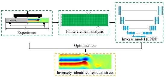
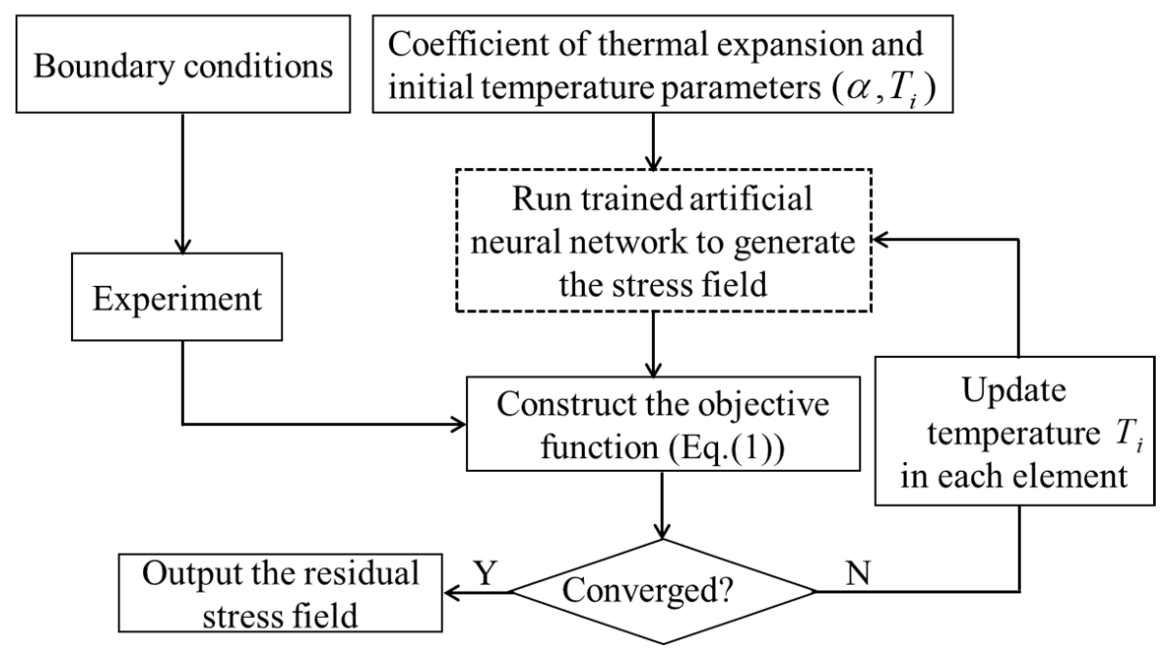
2.1. Inverse Strategy

The inverse problem is essentially an optimisation problem, which aims to minimise the difference between the simulation and experimental results. The FEMU method is one of the commonly used inverse methods and has been successfully applied to the parameter identification of a variety of materials. However, owing to the complexity of the finite element method in calculating residual stress, the inverse approach based on the FEMU method is rarely used for residual stress determination. In this paper, an inverse method using a neural network is proposed to replace the finite element program. Without compromising accuracy, this method can not only determine the complete residual stress distribution base on the stress values of finite measuring points, but also reduce the calculation time dramatically.

To obtain the residual stress of structural components under different process and boundary conditions, selecting the appropriate inverse parameters is of prime importance. In a thermal analysis, when the element temperature and coefficient of thermal expansion are provided, the finite element model can generate a stress field satisfying the self-equilibrium equation. Based on this, complex and diverse stress fields can be realised by applying random temperature and coefficient of thermal expansion at the integration point of each element in a finite element model. However, it should be noted that the temperature field in this method is fictitious and is only used as a means to obtain the residual stress, or to simulate any process conditions that produce the residual stress field. To determine the residual stress field, the optimisation task of this study is to determine the temperature distribution which can minimise the difference between the measured residual stresses and the inversely calculated residual stresses under a particular coefficient of thermal expansion. In fact, when the material properties are provided, the optimisation algorithm can always find a temperature field satisfying the convergence criterion of the objective function by adjusting the temperatures of the elements. Therefore, in this inverse method, all parameters are set as given constants except the element temperature.

To minimise the difference between the inversely calculated and measured residual stresses, the objective function was established as follows:

$$Q={{\displaystyle \sum _i^N\left[{\displaystyle \sum _j^M{({\sigma }_j^{CNN}(T_i,\alpha )-{\sigma }_j^{EXP}(T_i,\alpha ))}^2}\right]}}_i/N$$

(1)

where α and T_i are the coefficient of thermal expansion and element temperature, respectively, N is the total number of measured points and M represents the number of stress components. For a planar problem, the stress components include σ_x, σ_y and τ_xy, so M = 3. Further, ${\sigma }_j^{CNN}$ is the stress at the integration point of each element calculated by neural network and ${\sigma }_j^{EXP}$ is the measured residual stress at the corresponding position.

Figure 1 shows the flow chart of the inverse method based on the CNN. The inverse strategy mainly includes three steps, residual stress measurement, CNN establishment and parameter optimisation. For the first step, to verify the proposed inverse method, the stress field created by a simulated four-point bending experiment of an elastic-plastic material was used as the residual stress field in this paper. The second step involves a series of skills such as pre-processing, training and post-processing of the neural network. In the final step, the optimisation algorithm is used to update the temperature in each element to minimise the objective function (Equation (1)).

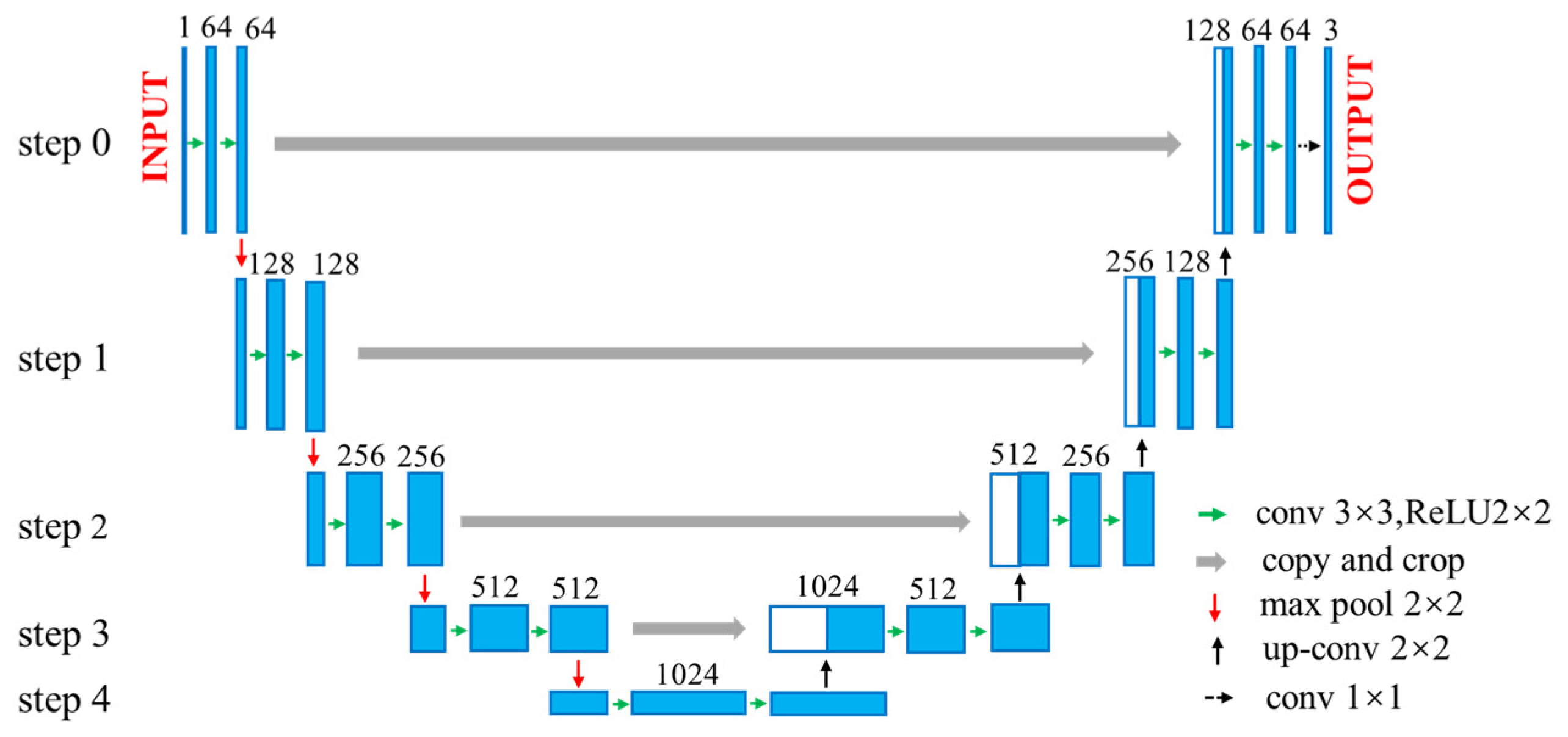
2.2. U-Net Architecture

The U-Net architecture is a typical U-shaped CNN architecture, which was proposed by Ronneberger et al. [22] for medical image segmentation. It exhibits excellent prediction accuracy among similar networks. As shown in Figure 2, the U-Net framework is symmetric. It is similar to an automatic encoder with an encoding path that converts the input space into a low-dimensional representation and a decoding path that extends it back to the original size [23]. The encoding path contains four down-sampling steps (steps 0, 1, 2 and 3), each consisting of two 3 × 3 convolution operations followed by a pooling operation with a stride of 2. Thus, the convolution layer learns the mechanical response of different temperature fields, such as stress fields. In each step, the number of channels doubles and the size of the feature map halves. Channels are used to store feature maps and each channel stores a feature map. At the bottom of the network, there are two 3 × 3 convolution layers connecting the encoder to the decoder. Moreover, similar to the encoding path, the decoding path also consists of four steps, with each step including an up-sampling 2 × 2 transposed convolution and two padded 3 × 3 convolutions. Simultaneously, the feature maps from the encoding path are cropped and connected to the up-sampled feature maps to complete the information fusion. In the decoding part, the numbers of feature maps and channels are halved in each step, but the size of the feature map is doubled. Finally, a 3 × 3 convolution operation converts the feature maps to three output channels, that is, three stress components are stored in three channels, respectively. The number of the feature maps controls the prediction accuracy of the network and a higher number of feature maps can deal with more complex problems. Consequently, on comparing the prediction effects of different number of feature maps, it was observed that, when the number of feature maps was equal to 128 or 256, the prediction performance was the best.

2.3. Database and U-Net Training Strategy

Sufficient data are the key to ensure the high-precision prediction ability of the neural network and finite element software is one of the primary sources to generate large datasets. In fact, once the finite element model is established with given material parameters, the dataset can be obtained by applying random temperatures to the element integration points. To render the training and verification dataset more universal, the Latin cube sampling method [25] was used to design the virtual experiment of variable space, wherein the range of a variable was divided into several intervals and one number was randomly selected from each interval to form a sample. This helped to evenly distribute the variable values in the whole variable space. In this study, the element temperature is the variable to be optimised and its upper and lower limits depend on the magnitudes of actual residual stresses and can be determined by the trial and error method. After determining the temperature range, the Latin cubic sampling method is used to divide the temperature range into several intervals with its number equal to the sample size. Subsequently, the temperature and corresponding stress components of each element can be extracted from the dataset.

Different evaluation indexes have different dimensions and units, which may affect the result of data analysis. To avoid this, the dataset was normalised using Equation (2).

$$x^{*}=\frac{x-\overline{x}}{s}$$

(2)

where $x$ is the original datum and $\overline{x}$ and $s$ represent the mean and standard deviation of the dataset, respectively.

Based on Keras [26], a deep learning library of Python, the U-Net architecture was constructed and tested. When training the network, the MSE (Equation (1)) was used as the error function and the Adam optimiser was employed. Further, the learning rate for the network was set as 10⁻⁵ with ReLU used as the activation function and the training number was equal to 1000.

3. Results

In this section, we present how, first, the target residual stress field was obtained via simulated four-point bending experiments of elastic-plastic aluminium alloy. Thereafter, a four-point bending CNN model based on the U-Net was established and the influence of dataset size on the prediction accuracy of the model was analysed. Finally, the effect of the number of measured points on the inverse accuracy of the residual stress field was studied.

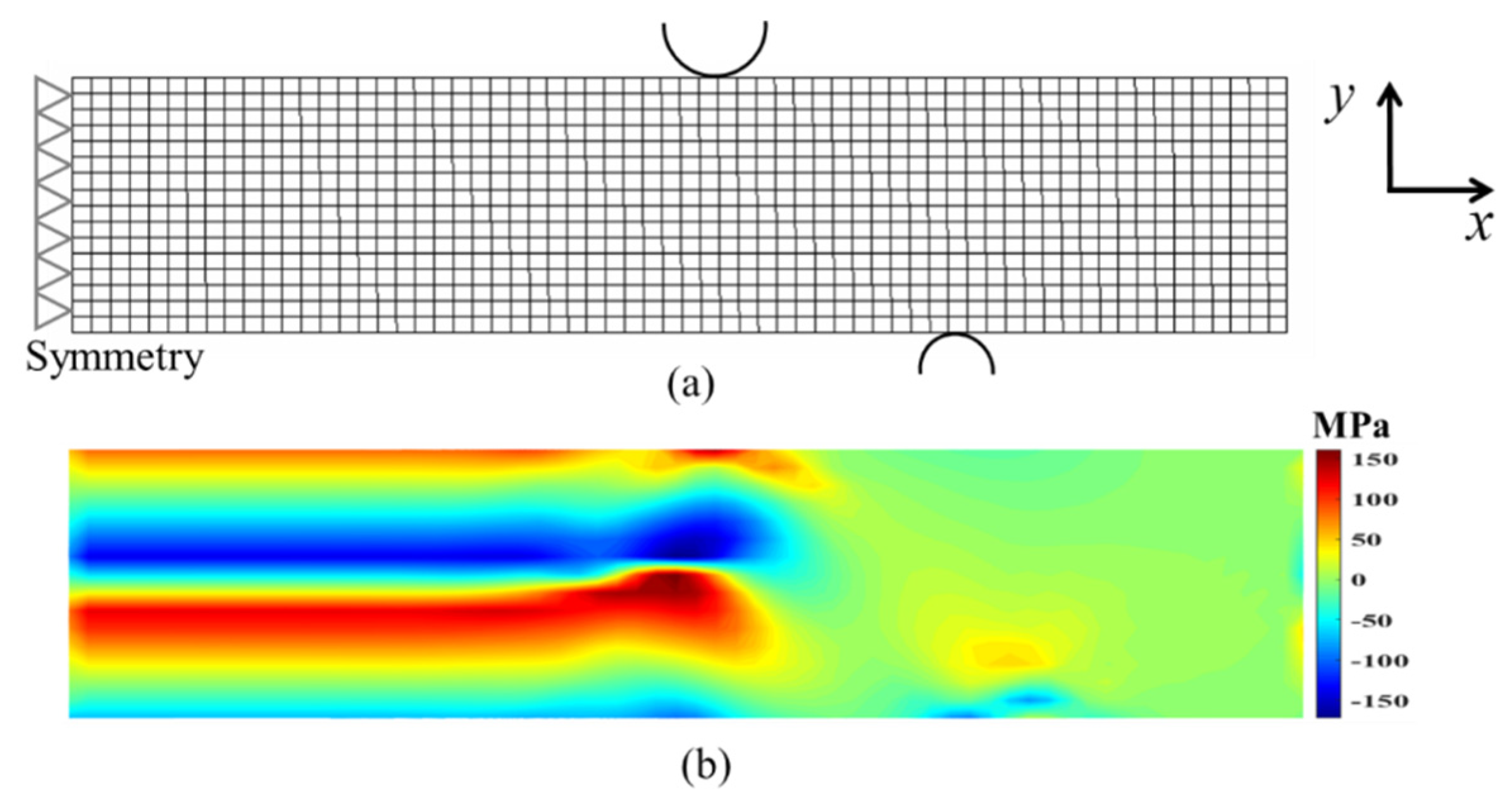
3.1. Residual Stress Field of Simulated Four-Point Bending Experiment

As shown in Figure 3a, a two-dimensional four-point bending finite element model with the size of 100 mm × 20 mm was created using ABAQUS software. Owing to the symmetry of the load and structure, only one half of the bending beam was modelled, while the symmetric boundary condition was applied on the left of the model. Further, the supporting cylinder at the bottom and the loading cylinder on the top were established as analytical rigid bodies. The finite element model was discretised into 1024 plane stress elements (CPS4R in ABAQUS) with 64 elements along the horizontal direction and 16 elements along the vertical direction. The beam was assigned with ideal elastic-plastic material properties with an initial elastic modulus of 70 GPa, Poisson’s ratio of 0.3 and a yielding stress of 200 MPa. Moreover, a prescribed vertical displacement with the magnitude of 10 mm was applied at the reference point of the loading cylinder to make the beam yield. Subsequently, the beam was completely unloaded and then the stress field existing in the beam was regarded as the actual residual stress field. Figure 3b shows the actual residual stress field in the horizontal direction (σ_x). It is evident that the residual stress was mainly distributed in the pure bending part of the beam.

3.2. Residual Stress Prediction Based on UNet Architecture

The U-Net architecture accepts images as its input and output. The length and width of the images (in pixels) are equal to the number of elements along the horizontal and vertical directions of the finite element model, respectively. Each pixel in the image represents the element temperature or stresses at the integration point position of the finite element. Different from the classification problems, the regression U-Net architecture established in this paper needed to output the stress components of each element. For the model in Figure 3, the numbers of input and output variables were 1024 (element temperature T) and 3072 (stress components σ_x, σ_y and τ_xy), respectively. Owing to the multitude of variables, successful training of the neural network was a challenge. However, to improve the prediction accuracy, this large-scale prediction task was decomposed into multiple sub-tasks. Task decomposition was divided into two steps. In the first step, the whole image was divided into four sub-images labelled as ①–④, that is, the four black bold line boxes as shown in Figure 4, with each sub-image containing 16 × 16 pixels. However, edges were produced between sub-images after image segmentation and large errors were caused when the neural network learned the image features due to the lack of pixels near these edges. Consequently, to diminish this edge effect, three more sub-images with the same size (16 × 16 pixels), that is, the red dash line boxes labelled as ⑤–⑦ in Figure 4, were created in the second step. Moreover, the edges generated in the first step should be located in the middle of the red sub-images as far as possible. Following this processing, seven networks were to be trained. Further, when the model needed to be restored to its original size after the neural network learning for each sub-image, the pixel values on the segmentation edges of sub-images ①–④ were overwritten by those at the same positions of sub-images ⑤–⑦.

According to the four-point bending simulation results shown in Figure 3b, the range of residual stress was from −200 to 200 MPa. For an assumed coefficient of thermal expansion (1.5 × 10⁻⁵/°C), the temperature range of elements was determined to be from −130 °C to 130 °C via the trial and error method. In this work, the dataset was obtained by providing different temperature fields in the finite element model and extracting the corresponding stress fields. In total, 80% of the dataset was used to train the CNN model and the remaining 20% was used for model verification. However, the size of the dataset has an important effect on the prediction accuracy of a model. Too small a dataset results in insufficient model feature learning, while too large a dataset causes very long model training time. Therefore, to determine the appropriate size of dataset, three analyses were performed with dataset sizes equal to 8260, 10,260 and 12,260, respectively. Figure 5 shows the root-mean-square errors (RMSE) for model verification of the three analyses. The RMSE was defined as

$$F=\sqrt{Q}$$

(3)

where Q is calculated using Equation (1). It is evident, from Figure 5, that the dataset size used in this paper had a slight effect on the prediction accuracy of the model, indicating that the amount of data required for neural network learning was reached. In contrast, the RMSE was the smallest when the dataset size was 10,260; thus, the subsequent study will be conducted based on this dataset.

Only the residual stresses at a finite number of points can be measured by experimental testing and it is very important to inversely determine the full-field residual stress according to the measured results at these points [27]. To study the influence of the number of measurement points on the full-field residual stress prediction, four cases were considered with the number of measurement points (elements) equal to 1024, 768, 512 and 448, respectively. The positions of these measurement points are shown in

Table 1. Locations of measurement points (elements).

Measurement Points	1024	768	512	448
Row	1:1:16	1:2:16; 2:2:16	1:1:16	1:1:16
Column	1:1:64	1:1:64; 1:2:64	1:2:64	1:2:40; 41:3:64

. Row and Column represent the positions of elements with known residual stresses at their integration points according to the rule of “start:step:end”. For example, “1:2:16” in Row represents the elements in the 1st row, the 3rd row (...) and the 15th row of the mesh (Figure 3a). Figure 6 shows the inversely determined residual stress fields based on different numbers of measurement points. It can be observed that the four cases with different numbers of measurement points yielded quite similar residual stress contours to the simulated experimental result in Figure 3b, except for the stress distribution at the edges of the model. The reason for the relatively large errors at the edges may be that, during the network training process, the pixels near the edges were lost in each convolution, resulting in insufficient learning of the features. Further, to compare the predicted residual stress field with the simulated experimental result more intuitively, the relative error among them is shown in Figure 7. The relative error is defined as the difference between the predicted and experimental values divided by the experimental value. In Figure 7, the abscissa represents the actual residual stresses of all elements in Figure 3b, while the ordinate represents the relative error. It is evident that the larger the absolute value of residual stress, the smaller the error and the residual stresses of most elements with error greater than 20% were close to zero. This is reasonable because, for a small residual stress, a small deviation yields a huge relative error. Figure 8 shows the relative errors of elements with stress exceeding 20 MPa versus the proportion of elements with relative errors larger than a specified value. It can be observed that, with the decrease in the number of measurement points, the relative error increased sharply. For 1024 measurement points, the ratio of elements with relative error larger than 20% was only 1.42%. However, when the number of measurement points was reduced to 448, the ratio of elements with relative error larger than 20% increased to 12.56%. In fact, the elements with large errors were mainly located at the edges of the model. This is mainly due to the insufficient learning caused by the lack of pixels when the neural network learned the edge features. Some image processing methods could be used to improve this in the future.

4. Discussion

In this section, the stability of the inverse algorithm under different initial values is studied and the efficiencies of the inverse methods based on U-Net and traditional FEMU are compared.

4.1. Influence of Initial Values on Stability of the Inverse Algorithm

A stable algorithm should provide stable results under different data disturbances, which is crucial to the reliability of the algorithm. In general, the stability of the algorithm is examined using different initial values. In the optimisation process of this study, the normalized temperatures of all elements were set as a constant T (0 ≤ T ≤ 1), which was then mapped to the input range of the network using Equation (4).

$$T^{*}=(T_{\max }-T_{\min })T+T_{\min }$$

(4)

where T* represents the input temperature of the elements for the neural network and T_max and T_min were set at 130 °C and −130 °C, respectively, as stated in Section 3.2. From

Table 2. RMSE and iterations of the inverse algorithm under different initial values.

Initial Values	0.2	0.5	0.8
RMSE (MPa)	7.82	7.45	7.61
Iteration times	2.5 × 106	106	2.3 × 106

, it is evident that, when different initial normalized temperature values (0.2, 0.5 and 0.8) were used for the inverse algorithm, similar accuracies could be achieved after enough iterations. However, the initial values affected the computational efficiency and T = 0.5 yielded the least number of iterations among the three cases studied.

4.2. Comparison of CPU Running Time of Different Inverse Algorithms

The inverse method proposed in this study used a CNN to replace the FEMU used in the conventional inverse method. The efficiencies of these two methods were compared by considering the case of T = 0.5 in Table 2 as an example. The inverse problems were simulated on a computer configured with a quad-core 2.6 GHz CPU, but only one CPU was used without parallel computing.

Table 3. Comparison of running time between CNN- and FEMU–based methods.

Procedure	Time
	CNN-Based	FEMU-Based
Each iteration	0.08 s	21 s
Training	22.91 h	0
Sampling	59.85 h	0
Total	82.76 h	5833.33 h (estimated)

presents the time required for the CNN- and FEMU-based methods to complete one iteration. The time used for the FEMU-based method was 21 s, while the CNN-based method only required 0.08 s, which is almost negligible compared to the former. Totally, 10⁶ iterations were needed for the CNN-based method to obtain the converged result. Including the training and sampling time, the whole optimisation task took about 82.76 h for the CNN-based method, while it seemed to take forever for the FEMU method. If the same number of iterations was assumed for the two methods, the estimated time for the FEMU-based method would be 5833.33 h, which is far more than that of the CNN-based method. Therefore, it can be concluded that the proposed CNN-based inverse method significantly outperformed the conventional one in terms of computational efficiency.

5. Conclusions

The efficient prediction of the full-field residual stress from a limited number of measurement points is still a challenging task. However, by replacing the FEMU technique in the conventional inverse method with a CNN, a novel inverse method is proposed in this paper to determine the residual stress field of structural components. The main conclusions are as follows:

(1)

The machining process and conditions of structural components need not be known and the full-field residual stress satisfying mechanical constrains can be inversely determined from limited measurement points.

(2)

In the proposed method, the U-Net architecture trained by the temperature and stress fields exhibited superior performance in predicting residual stress field and greatly improved the computational efficiency. In fact, the residual stress determined by this method reached an accuracy close to that of the X-ray diffraction method.

(3)

Moreover, the proposed inverse method based on neural networks is not only suitable for the residual stress prediction but can also undertake inverse identification of various material parameters such as damage factors.

References

1. Akhtar, N.; Afzal, M.; Awais, M.; Akbar, M. Optimizing cold compression deformation to remove residual stresses in die forged disc of Al-Mg-Si alloy. Key Eng. Mater. 2018, 778, 53–60. [Google Scholar] [CrossRef]
2. Tao, X.; Gao, Y. Influences of thermal effects on residual stress fields of an aluminium-lithium alloy induced by shot peening. Int. J. Adv. Manuf. Technol. 2021, 112, 3105–3116. [Google Scholar] [CrossRef]
3. Wang, Y.; Peng, R.L.; Wang, X.-L.; McGreevy, R. Grain-orientation-dependent residual stress and the effect of annealing in cold-rolled stainless steel. Acta Mater. 2002, 50, 1717–1734. [Google Scholar] [CrossRef]
4. Li, X.; Qi, C.; Zhang, P. A micro-macro confined compressive fatigue creep failure model in brittle solids. Int. J. Fatigue 2020, 130, 105278. [Google Scholar] [CrossRef]
5. Zhang, Z.; Tan, Q.; Cui, Y.; Tian, Y.; Wang, Y.; Qin, H.; Bi, Z.; Wang, Y. Experimental validation of residual stress thermomechanical simulation in as-quenched superalloy discs by using diffraction and incremental hole-drilling methods. Mater. Today Commun. 2021, 27, 102229. [Google Scholar] [CrossRef]
6. Gadallah, R.; Tsutsumi, S.; Yonezawa, T.; Shimanuki, H. Residual stress measurement at the weld root of rib-to-deck welded joints in orthotropic steel bridge decks using the contour method. Eng. Struct. 2020, 219, 110946. [Google Scholar] [CrossRef]
7. Zhu, K.Y.; Li, Z.Q.; Fan, G.L.; Xu, R.; Jiang, C.H. Thermal relaxation of residual stress in shot-peened CNT/Al–Mg–Si alloy composites. J. Mater. Res. Technol. 2019, 8, 2201–2208. [Google Scholar] [CrossRef]
8. Marciszko, M.; Baczmański, A.; Klaus, M.; Genzel, C.; Oponowicz, A.; Wroński, S.; Wróbel, M.; Braham, C.; Sidhom, H.; Wawszczak, R. A multireflection and multiwavelength residual stress determination method using energy dispersive diffraction. J. Appl. Crystallogr. 2018, 51, 732–745. [Google Scholar] [CrossRef] [Green Version]
9. Marola, S.; Bosia, S.; Veltro, A.; Fiore, G.; Manfredi, D.; Lombardi, M.; Amato, G.; Baricco, M.; Battezzati, L. Residual stresses in additively manufactured AlSi10Mg: Raman spectroscopy and X-ray diffraction analysis. Mater. Des. 2021, 202, 109550. [Google Scholar] [CrossRef]
10. Schoderböck, P.; Köstenbauer, H. Residual stress determination in thin films by X-ray diffraction and the widespread analytical practice applying a biaxial stress model: An outdated oversimplification? Appl. Surf. Sci. 2020, 541, 148531. [Google Scholar] [CrossRef]
11. Faghidian, S.A. New framework for Bayesian statistical analysis and interpolation of residual stress measurements. Mech. Res. Commun. 2013, 50, 17–21. [Google Scholar] [CrossRef]
12. Jiang, X.; Li, H.; Wang, Y.; Ding, Z. An approach to predict the distortion of thin-walled parts affected by residual stress during the milling process. Int. J. Adv. Manuf. Technol. 2017, 93, 4203–4216. [Google Scholar] [CrossRef]
13. Oliveira, A.L.R.D.; Rego, R.R.; de Faria, A.R. Residual stresses prediction in machining: Hybrid FEM enhanced by assessment of plastic flow. J. Mater. Process. Technol. 2020, 275, 116332. [Google Scholar] [CrossRef]
14. Chukkan, J.R.; Wu, G.; Fitzpatrick, M.E.; Jones, S.; Kelleher, J. An iterative technique for the reconstruction of residual stress fields in a butt-welded plate from experimental measurement, and comparison with welding process simulation. Int. J. Mech. Sci. 2019, 160, 421–428. [Google Scholar] [CrossRef]
15. Jun, T.-S.; Korsunsky, A.M. Evaluation of residual stresses and strains using the Eigenstrain Reconstruction Method. Int. J. Solids Struct. 2010, 47, 1678–1686. [Google Scholar] [CrossRef] [Green Version]
16. Markiewicz, É.; Langrand, B.; Notta-Cuvier, D. A review of characterisation and parameters identification of materials constitutive and damage models: From normalised direct approach to most advanced inverse problem resolution. Int. J. Impact Eng. 2017, 110, 371–381. [Google Scholar] [CrossRef]
17. Liu, G.; Wang, L.; Yi, Y.; Sun, L.; Shi, L.; Ma, S. Inverse identification of graphite damage properties under complex stress states. Mater. Des. 2019, 183, 108135. [Google Scholar] [CrossRef]
18. Aguir, H.; Belhadjsalah, H.; Hambli, R. Parameter identification of an elasto-plastic behaviour using artificial neural networks–genetic algorithm method. Mater. Des. 2011, 32, 48–53. [Google Scholar] [CrossRef]
19. Ali, U.; Muhammad, W.; Brahme, A.; Skiba, O.; Inal, K. Application of artificial neural networks in micromechanics for polycrystalline metals. Int. J. Plast. 2019, 120, 205–219. [Google Scholar] [CrossRef]
20. Zhang, Y.; Sun, G.; Xu, X.; Li, G.; Huang, X.; Shen, J.; Li, Q. Identification of material parameters for aluminum foam at high strain rate. Comput. Mater. Sci. 2013, 74, 65–74. [Google Scholar] [CrossRef]
21. Fan, J.; Xu, W.; Wu, Y.; Gong, Y. Human Tracking Using Convolutional Neural Networks. IEEE Trans. Neural Netw. 2010, 21, 1610–1623. [Google Scholar] [CrossRef] [PubMed]
22. Ronneberger, O.; Fischer, P.; Brox, T. U-Net: Convolutional Networks for Biomedical Image Segmentation, International Conference on Medical Image Computing and Computer-Assisted Intervention; Springer: Berlin/Heidelberg, Germany, 2015; pp. 234–241. [Google Scholar]
23. Mendizabal, A.; Márquez-Neila, P.; Cotin, S. Simulation of hyperelastic materials in real-time using deep learning. Med. Image Anal. 2020, 59, 101569. [Google Scholar] [CrossRef] [PubMed]
24. Koeppe, A.; Bamer, F.; Markert, B. An intelligent nonlinear meta element for elastoplastic continua: Deep learning using a new Time-distributed Residual U-Net architecture. Comput. Methods Appl. Mech. Eng. 2020, 366, 113088. [Google Scholar] [CrossRef]
25. Donovan, D.; Burrage, K.; McCourt, T.; Thompson, B.; Yazici, E. Estimates of the coverage of parameter space by Latin Hypercube and Orthogonal Array-based sampling. Appl. Math. Model. 2018, 57, 553–564. [Google Scholar] [CrossRef] [Green Version]
26. Chollet, F. Keras: The Python Deep Learning Library. Astrophysics Source Code Library. 2018. Available online: https://github.com/keras-team/keras (accessed on 7 December 2021).
27. Coules, H.; Smith, D.; Venkata, K.A.; Truman, C. A method for reconstruction of residual stress fields from measurements made in an incompatible region. Int. J. Solids Struct. 2014, 51, 1980–1990. [Google Scholar] [CrossRef] [Green Version]
Figure 1. Flow chart of the inverse method.
Applsci 12 01195 g001
Figure 2. U-Net architecture.
Applsci 12 01195 g002
Figure 3. Fourpoint bending model and simulated residual stress field: (a) four-point bending model; (b) simulated residual stress field ( σ x ).
Applsci 12 01195 g003
Figure 4. Sub-images in task decomposition:①–⑦ represents seven sub-images.
Applsci 12 01195 g004
Figure 5. Influence of dataset size on prediction accuracy of U-Net.
Applsci 12 01195 g005
Figure 6. Residual stress fields ( σ x ) by inverse identification: (a) 1024 measurement points, (b) 768 measurement points, (c) 512 measurement points and (d) 448 measurement points.
Applsci 12 01195 g006
Figure 7. Relative error versus element stress.
Applsci 12 01195 g007
Figure 8. Relative error versus ratio of elements.
Applsci 12 01195 g008