Analysis of a Cardiac-Necrosis-Biomarker Release in Patients with Acute Myocardial Infarction via Nonlinear Mixed-Effects Models ^†

Abstract

The release of the cardiac troponin T (cTnT) in patients with acute myocardial infarction (AMI) has been analyzed through a methodology based on nonlinear mixed-effects (NME) models. The aim of this work concerns the investigation of any possible relationship between clinical covariates and the dynamics of the release of cTnT to derive more detailed and useful clinical information for the correct treatment of these patients. An ad-hoc mechanistic model describing the biomarker release process after AMI has been devised, assessed, and exploited to evaluate the impact of the available clinical covariates on the cTnT release dynamic. The following approach was tested on a preliminary dataset composed of a small number of potential clinical covariates: employing an unsupervised approach, and despite the limited sample size, dyslipidemia, a known risk factor for cardiovascular disease, was found to be a statistically significant covariate. By increasing the number of covariates considered in the model, and patient cohort, we envisage that this approach may provide an effective means to automatically classify AMI patients and to investigate the role of interactions between clinical covariates and cTnT release.

1. Introduction

Current trends in the diagnostic field make use of increasingly sophisticated techniques based on the analysis of circulating biomarkers: these techniques, in addition to their specificity and sensitivity, are also minimally invasive since they are based on sample blood analysis. For example, several cardiac biomarkers are released into circulation following stress on cardiac function or damage to myocardial tissue. In particular, among these, the measurements of specific cardiac biomarkers, such as the cardiac troponins T (cTnT) and I (cTnI), are currently exploited to diagnose and confirm the presence of acute myocardial infarction (AMI): this condition represents one of the most frequent and severe acute coronary syndrome (ACS), associated with insufficient blood supply and, finally, death of the involved cardiac tissue, [1]. More recently, especially with the advent of the high-sensitivity tests for cardiac troponins, their use has extended beyond the diagnosis of AMI, to encompass clinical risk stratification and prognostic assessment, [2]. Several factors, such as gender, age, and circadian cycle, [3,4,5], influence the release of cTns. For this reason, in this work, we are interested in investigating and modeling the impact of such available clinical covariates on the release dynamic of cTns, in particular of cTnT, in order to derive more detailed and better performing simulation models. To this end, we exploit the flexible modeling approach of the nonlinear mixed-effects (NME) models to describe the response of a dynamic system by taking into account both the influence of fixed and random effects, with the possibility to include the effects of the covariates directly in the model. This approach is especially suitable to deal with repeated experimental measurements on different subjects, e.g., balanced and unbalanced longitudinal datasets, and with missing data, [6,7]. Furthermore, NME models allow the exploitation of all the possible information available in the experimental set, in order to improve the quality of the model results. Similarly to the classic nonlinear regression approach, [8,9,10,11], mixed-effects models find wide application in various biological fields and especially in pharmacokinetics. As an example, in [12], NME models are applied to collect clinical data on 59 newborns treated with phenobarbital, in the first 16 days after birth, in order to investigate how to improve the dosing phase of the drug, optimizing the therapy. Another popular trend concerns the application of NME to model the growth in cellular species, [13], and the dynamics of the concentration of molecular species in a biological compartment [14,15]. In the clinical setting as well, the NME models show their great potential: e.g., Samson et al., in [16], leveraged NME models to describe the reduction in viral load after the initiation of treatment and to evaluate the intra- and inter-patient variability in the HIV clinical trials. French et al., in [17], applied ME models to identify key parameters in datasets of diabetic patients with foot ulcers: the identification of such parameters proved especially useful for diagnosis and treatment. In [18], Ieva et al. used the nonlinear semi-parametric and parametric ME model to detect different patterns of growth in the number of NSTEMI diagnoses, with the aim of monitoring the diffusion of new diagnostic techniques.

As mentioned above, in this work, NME models are applied to analyze a dataset of patients subject to acute myocardial infarction with ST-segment elevation (STEMI). In particular, we are interested in evaluating the effect of the available clinical covariates on the evolution of cTnT plasmatic concentration, with the aim of identifying different sub-classes of STEMI patients. The main advantage of a computer-aided classification of patients may consist in the possibility to optimize both the diagnosis and the treatment of these patients and to maximize the added value of the use of cardiac-necrosis biomarkers to assess prognosis. The stochastic approximation expectation maximization (SAEM) algorithm is chosen to perform the identification of the model parameters and to evaluate the impact of the available clinical covariates. The reason for choosing SAEM lies in the peculiarity of the experimental measurements, which appear temporally dependant on the time of onset of AMI: even though the distance between two subsequent acquisitions is approximately the same among different patients, the time elapsed from the infarct until the first acquisition is different for each patient, due to a number of factors (e.g., the severity of the pain, closeness to the hospital). In this regard, our recent work explored the feasibility of estimating the onset time of the AMI using cTnT curves in those cases where this information was not available or unreliable, [19]. Furthermore, the measurements are very heterogeneous in terms of concentration: the troponin levels in the blood are heavily affected by the extent of the damage, and, in STEMI patients, by the type of pharmacological treatment they have undergone before the measurements (e.g., thrombolysis).

A preliminary version of the present work has been presented in [20]; the present work has been improved and extended in several directions: firstly, the analysis was conducted on a more comprehensive set of clinical covariates, including, e.g, age, gender, and AMI onset time, which were not considered in the previous work. In particular, the impact of the AMI onset time on the release dynamics of cTnT has been carefully examined in this work. The parameters-identification step has also been improved by exploiting two different identification phases (one of which relies on simulated annealing). The reliability of the obtained results and the robustness of the technique were tested and suitably validated from a statistical point of view. In addition to the results, the background and methods sections have also been significantly expanded in the present version of the paper.

The paper is structured as follows: Section 2 provides the background on the NME models, and on the AMI pathophysiology, while Section 3 is dedicated to describing the exploited mathematical model and the available clinical data. Section 4 presents the results, followed by discussion in Section 5.

2. Background

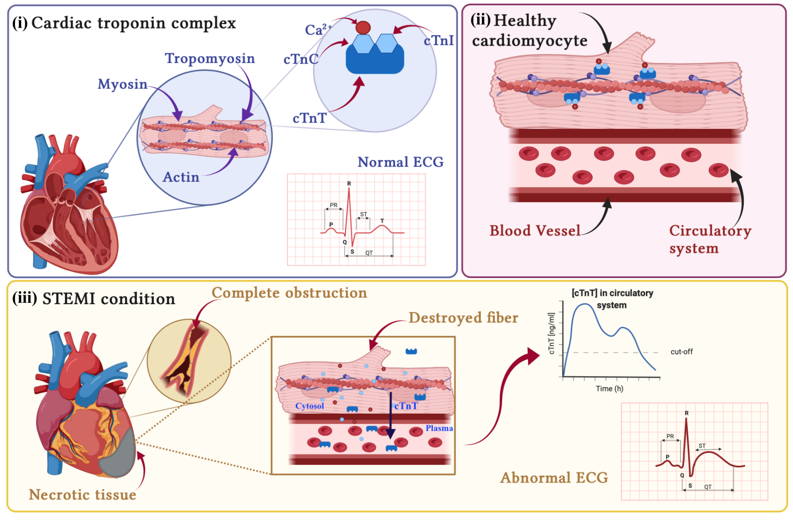
2.1. Pathophysiology of AMI

Cardiac troponins are a protein complex involved in the contraction of the cardiac muscle. They are composed of three different subunits, (i) cardiac troponin C (cTnC), (ii) cardiac troponin I (cTnI), and (iii) cardiac troponin T (cTnT), Figure 1(i). In the presence of an electrical stimulus, the cell is activated, causing a rapid increase in the intracellular concentration of Ca²⁺, which can bind cardiac troponin C (cTnC), favoring conformational changes in tropomyosin. As a result, the myosin and actin filaments are free to slide over each other, allowing the muscle fibers to contract. In a healthy cardiomyocyte, Figure 1(ii), the integrity and functionality of all fibers and of the protein complex are maintained: therefore, the concentration of cTnT is undetectable in peripheral blood.

After the onset of AMI, the blood flow downstream of the obstruction impedes the normal blood supply to the underlying tissue, causing its death; see Figure 1(iii). At the cellular level, the necrosis of this tissue implicates the progressive desegregation of the fibers, and the diffusion of cTns subunits from the disrupted sarcomere, first into the cytosol, and then into the plasma, where it is possible to measure the concentration levels of the cTns through specific assays; see Figure 1(iii). In the plasma of AMI patients, cTnT concentrations describe a typical biphasic curve, see Figure 1(iii), in which the first peak is due to the early and rapid leakage of the cTnT molecules contained in the cytoplasm, following the rupture of the outer cell membrane, while the second one is due to the slow release of the sarcomeric cTnT, following the degradation of the cardiac fibers. It is possible to characterize two main clinical classes of AMI patients, which require different approaches in both diagnosis and treatment. These classes are represented by:

• STEMI (ST-segment elevation AMI): in this class of patients, the obstruction usually completely blocks the blood supply to the tissues downstream of it. In this case, the extension of the cardiac damage is such that it causes alterations in the electrical activity of the heart, resulting in a visible elevation of the ST-segment on the ECG, [21]; see Figure 1(iii).
• NSTEMI (non-ST-segment elevation AMI): the occlusion is only partial; therefore, a reduced blood flow is guaranteed downstream of the obstruction; these patients exhibit an ECG without visible alteration [22].

In the present study, we focus our attention on STEMI patients, since the release profile and its dynamic are well-known from a clinical point of view, [23,24], with the possibility to associate a specific mathematical behavior. Indeed, for this class of patients, we were able to define an ad-hoc mathematical model able to reconstruct the release profile of cardiac troponin T (cTnT) in the plasma.

2.2. Nonlinear Mixed-Effects Models

A generic representation of a nonlinear model,

$$y_{ij}=f({\mathsf{\Phi }}_i,x_{ij})+e_{ij}$$

(1)

describes the jth response of the ith individual, expressed as a nonlinear function, f, of the predictor vector, $x_{ij}$, and the r-parameter vector, ${\mathsf{\Phi }}_i$, and with a measurement or process error given by $e_{ij}$, usually assumed to be independent and identically normally distributed, $\mathcal{N}(0,{\sigma }^2)$, where ${\sigma }^2$ represents the variance of the residual. The peculiarity of the ME lies in the parameter vector ${\mathsf{\Phi }}_i$, expressed as the combination of two types of effects (see [7,12,13]):

• Fixed effects—the terms, in the parameter expressions, that remain constant over all the individuals of the analyzed population. They represent the set of the population parameters.
• Random effects—the random components of the model parameters, assumed to be different among individuals or groups of individuals;

Therefore, we can rewrite the vector of individual parameters ${\mathsf{\Phi }}_i$ as follows:

$${\mathsf{\Phi }}_i=A_i\beta +B_i{\omega }_i$$

(2)

where $A_i$ and $B_i$ represent the covariate (or design) matrices for the $i-th$ subject for the fixed and random effects, respectively; $\beta$ is the p vector of the fixed population parameters; and ${\omega }_i\sim (0,{\sigma }^{2}D)$ is a q vector of random effects with covariance matrix equal to ${\sigma }^{2}D$ [7].

2.3. Stochastic Approximation Version of Expectation Maximisation Algorithm (SAEM)

In the present work, we exploited the stochastic approximation version of the expectation maximisation algorithm (SAEM), [25], with a Markov-chain Monte-Carlo procedure to investigate the implication of the available covariates on the release kinetics of cTnT in STEMI patients, as well as to estimate the model parameters. The expectation maximisation (EM) algorithm, [26], developed for problems with missing values, produces maximum-likelihood estimates (MLE) of the model parameters, and it consists of two main steps:

• Expectation step (E)—during which the likelihood of the observed data is computed starting from the current estimate of the model parameters;
• Maximization step (M)—where the estimate of the parameters is updated, seeking the point in the parameter space that maximizes the likelihood.

The EM algorithm is based on iterative executions of these two steps, until convergence. The SAEM algorithm introduces a stochastic approximation procedure, where the current approximation of the parameters depends on their a-posteriori density distribution, [27], and it is composed of (i) a first exploratory phase and (ii) a subsequent smoothing one. In particular, during the exploratory phase, Figure 2(i), the algorithm explores the parameter space, starting from an initialization point, and proceeding with two distinct steps, as follows:

(i)

The set of the individual parameters are computed by sampling a conditional distribution through Markov-chain Monte-Carlo procedure, namely

$$p\left({\mathsf{\Psi }}_i\right|y_i,{\theta }^k)$$

(3)

where ${\mathsf{\Psi }}_i$ represents the individual parameters set for subject i, $y_i$ is the experimental observation vector for subject i, and ${\theta }^k$ is the population parameters set at SAEM iteration k.

(ii)

the set of the population parameters is computed starting from the individual parameter sets identified at the previous iteration and represents the initialization point for a new exploratory iteration,

$${\theta }^{k+1}=\frac{1}{N}\sum _{i=1}^N{\mathsf{\Psi }}_i$$

(4)

The smoothing phase, Figure 2(ii), starts when the algorithm has moved in the region of the parameter space with a high probability of finding the optimal global solution. In this phase, the estimates are stabilized toward the maximum likelihood. As in the exploratory phase, the smoothing phase is composed of the two steps described above: however, in this case, the population parameters are computed taking into account the individual parameter sets identified in all the previous iterations of the smoothing phase,

$${\theta }^{k+1}=\frac{1}{k}\sum _{i=1}^k\frac{1}{N}\sum _{i=1}^N{\mathsf{\Psi }}_i$$

(5)

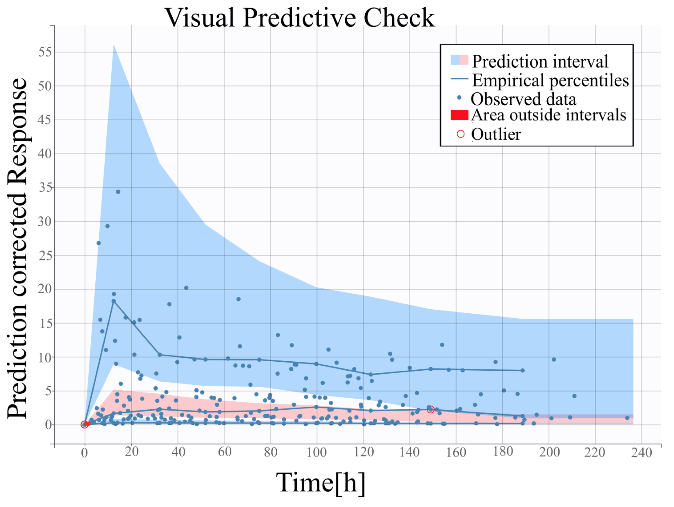
2.4. Visual Predictive Check

We evaluate the robustness of the proposed model and potential misspecifications in order to understand how the proposed model can interpret and correctly describe the observed process, i.e., providing accurate parameter predictions and avoiding inaccurate estimates. Many of the statistical methods used to assess the suitability of the model are based on graphical representation and they comprise ‘goodness-of-fit inspection methods’. These statistical techniques are simple to implement, but they can give misleading results when applied to non-linear mixed-effects models. Here, we choose to perform a visual predictive check (VPC), which allows us to evaluate the ability of the proposed model to reproduce both the central trend and the variability in the observed time-varying data [28]. VPC bases its analysis on performing several simulations, which are used to design the structure of the observed data. The first step consists of evaluating the empirical percentiles from the observed data in each temporal bin, allowing for a summary of their distribution. Then, the theoretical percentiles are computed from data generated by multiple Monte-Carlo simulations, and at the same temporal bins as the empirical ones. From these simulated replicas of the observed data, it is possible to generate non-parametric confidence intervals. The size of the confidence intervals allows for the evaluation of the real deviation between accurate observations and simulated data. In the VPC representation, the confidence intervals indicate the uncertainty of the predictions.

3. Materials and Methods

3.1. Nonlinear Model of Cardiac Troponin T (cTnT) Release in AMI Patients

Based on the abovementioned dynamics of an AMI, a three-compartmental model composed of three ordinary differential equations describing the variation in the concentration of the cardiac troponin T, cTnT, in sarcomere ($C_s$), cytosol ($C_c$), and plasma ($C_p$), was defined, [29,30,31], as follows:

$$\begin{array}{c}\hfill \left\{\begin{array}{cc}\hfill \frac{d{C}_s}{d\tau }& =-(C_s-C_c)\frac{{\tau }^3}{({\tau }^3+T_d^3)}\hfill \\ \hfill \frac{d{C}_c}{d\tau }& =(C_s-C_c)\frac{{\tau }^3}{({\tau }^3+T_d^3)}-a(C_c-C_p)\hfill \\ \hfill \frac{d{C}_p}{d\tau }& =a(C_c-C_p)-b{C}_p\hfill \end{array}\right.\end{array}$$

(6)

In model (6), the flux in cTnT between the three compartments, shown in Figure 1(iii), was modeled using Fick’s first law of diffusion, [32]. In particular, $a:=D_{cp}/D_{sc}$, $b:={\alpha }_{cp}/D_{sc}$, $T_d:=T/D_{sc}$, and $\tau :=D_{sc}t$ are the coefficient of diffusion between cytosol and plasma ($D_{cp}$), the clearance (${\alpha }_{cp}$), the time threshold for the sarcomeric disassembly ($T_d$), and the time, respectively, each one normalized by the coefficient of diffusion between sarcomere and cytosol ($D_{sc}$). Notably, model (6) is structurally identifiable, as in [33]: this property concerns the structure of the defined mathematical model and the choice of its parameters, and it was ensured by evaluating if the model was controllable and observable [34,35]. Finally, the output of the model is represented by the reconstructed cTnT concentration in the plasma, since only in this compartment it is possible to make measurements.

The implementation of the model, the estimation of the parameters, as well as all the statistical analysis were performed using Matlab and Monolix, [36], toolboxes.

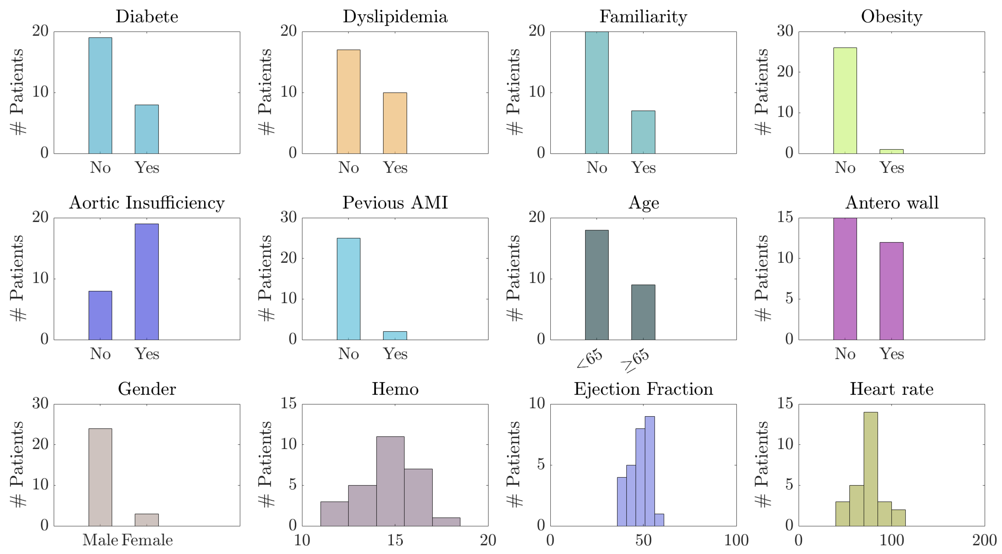
3.2. Experimental Dataset: cTnT Concentration Levels and Clinical Covariates

The experimental dataset exploited in the present study consists of a retrospective historical collection of time-series measurements of cTnT levels in the plasma of STEMI patients, provided by the Interventional Cardiology Unit of the Magna Graecia University Hospital in Catanzaro, Italy. The dataset includes some clinical information and biomarker measurements of 27 consecutive patients aged between 18 and 85 years, presented with STEMI and treated with percutaneous coronary revascularization (PTCA). Each blood sample was analyzed using highly sensitive assays (hs-cTnT) with a cut-off value of 0.014 [ng/mL], calculated on a reference population. According to the general guidelines, the first acquisitions were performed every 6 hours from the time of admission for the first one/two days, and then every 24 h, [22]. As previously mentioned, the dataset shows a high temporal inhomogeneity, mainly due to the fact that the time of the onset of symptoms varies from patient to patient, causing a mismatch between the acquisitions [19].

In addition, the experimental dataset contains several categories of clinical information, related to:

• Pre-hospital data: diabetes, dyslipidemia, smoke, obesity, familiarity with the disease (presence of cases of AMI in the family), and other cardiac pathologies;
• Admission data: time from onset of symptoms, gender, age;
• Post-hospitalization data: ejection fraction, thrombolysis, revascularization, biomarkers, anterior wall, and other information, along with data and time labels.

These covariates can be continuous, e.g., age, ejection fraction, and hemoglobin, or categorical, e.g., gender, dyslipidemia, diabetes, and smoke. Since the goal of the work is to investigate the influence of the clinical covariates on the cTnT release, we chose to not include all those covariates which can be identified as consequences rather than possible causes of an AMI, such as ejection fraction, hemoglobin, and anterior wall. Given the limited number of patients, and based on the indication suggested in [37] for the evaluation of the thrombolysis in myocardial infarction (TIMI) risk score for STEMI (an important predictor of mortality after AMI), we proceeded with the reorganization of the patients into two main groups based on their age (years): younger than 65, and older than 65. Figure 3 shows the distribution of all the categorical and continuous covariates exploited in the study.

Another crucial aspect to investigate is represented by the relationship between circadian rhythm and onset of AMI, which shows a peak of incidence of cases during the early morning, [38]. During this time interval, the oxygen demand increases with the vascular tone, while the coronary blood flow undergoes a decrease. This imbalance between supply and demand seems to have an impact on the onset of AMI symptoms, as reported in [39]. All the onset times can be grouped into four temporal bands over 24 h: (i) night ($0\le t_i<6$), (ii) morning ($6\le t_i<12$), (iii) afternoon ($12\le t_i<18$), and (iv) evening ($18\le t_i<24$). In our dataset, most patients present an indicative time of onset of symptoms at 00:00 ($0\le t_{AMI}<6$), arbitrarily chosen by clinicians following the inability to provide an estimation of this time by the patients. Since considering the onset of symptoms would imply a further reduction in the dataset (patients with AMI time at 00:00 cannot be included in the analysis), it was not taken into account in the present study. Informed consent was obtained by all patients.

3.3. Strategy for Covariates Selection

The high inter-individual variability can be dealt with by including the effect of the covariates in the troponin model (6). To identify which covariates among the available ones can better explain this variability, we statistically test the relationship between covariates and the model output. In particular, several models are tested following the pipeline reported below:

• A first analysis was performed without the introduction of covariates, in order to initialize the parameters identification phase.
• The effect of each covariate on the model parameters was assessed; Wald’s test was used to statistically evaluate which covariate yields a significant effect and should be added to the model. Bonferroni correction was applied to avoid the problem of multiple tests.
• Finally, the models obtained by the combination of the most significant covariates were analyzed.

The results are discussed in Section 4.

4. Results

4.1. Analysis of Selected Covariates

Table 1. Effects of the covariates on the parameters of model (6). M: model, PM: parameters of model (6) significantly influenced (the specific covariate is reported in square bracket), A: age, D: dyslipidemia, AI: aortic insufficiency. For each model, it is reported the effect of each covariate (in square brackets) on the parameters, and the associated p value computed via Wald’s test, and corrected for multiple tests using the Bonferroni.

M	Cov${}_1$	Cov${}_2$	Cov${}_3$	−2LL	BIC	SE	PM(Cov: ${\mathit{p}}_{\mathbf{val}}$)
1				−1613.80	−1576.76	0.655
2	D			−1651.87	−1569.93	0.427	b (D: $p=2.46\times {10}^{-5}$)
3	D	AI		−1655.09	−1604.58	1.575	b(D: $p=1.65\times {10}^{-7}$), T${}_d$(AI: $p=1.65\times {10}^{-9}$)
4	D	A		−1560.24	−1507.51	0.142	b(D,A: $p_D=5.5\times {10}^{-10}$,         $p_A=0.015$), $T_d$(A: $p=3.3\times {10}^{-15}$), $C_{s0}$(A: $p=3.3\times {10}^{-15}$)
5	A	AI		−1586.06	−1536.63	0.42	b(A,AI: $p_A=8.55\times {10}^{-10}$,         $p_{AI}=8.85\times {10}^{-5}$), $T_d$(A: $p=3.3\times {10}^{-15}$), $C_{s0}$(A: $p=3.3\times {10}^{-15}$)
6	A	AI	D	−1574.81	−1505.38	0.183	b(D: $p_D=4.2\times {10}^{-10}$), $T_d$(A,AI: $p=0.015$)

shows the results obtained for all the significant models, in terms of (i) log-likelihood, computed using importance sampling Monte-Carlo methods with a size of 10,000 samples, (ii) Bayesian information criterion (BIC) index, (iii) standard error (SE), and (iv) significance of the covariate influence on the model parameters, evaluated in terms of p-value.

In what follows, we focus our attention on model 2 of Table 1, which, besides exhibiting a good compromise of log-likelihood, BIC and SE, has been deemed of particular interest from the clinical standpoint; indeed, dyslipidemia is a known clinical cofactor in the incidence of AMI and, therefore, it is interesting to investigate its influence on the cTnT release curve.

The influence of dyslipidemia on parameter b was explicitly introduced in the model as follows:

$$log\left(b\right)=log\left(b_{pop}\right)+{\beta }_{b_{Dyslipidemi{a}_1}} \ast [Dyslipidemia=1]+{\omega }_b$$

(7)

where ${\beta }_{b_{Dyslipidemi{a}_1}}$ represents a part of the fixed effect, specific for the dyslipidemic class, and ${\omega }_b$ is the random effect specific to each individual. Since it is not possible to constrain the parameter values through the definition of specific bounds, whose values must be positive, we chose a log-normal distribution for the parameters, as shown in Equation (7).

Figure 4 shows the cTnT acquisitions of the 27 STEMI patients grouped according to the dyslipidemic covariate: the mean, the standard deviation, and the median values for the distribution of the experimental data are reported, for both dyslipidemic and non-dyslipidemic patients, in

Table 2. Mean, std, and median of cTnT concentration over the observation interval, for dyslipidemic and non-dyslipidemic patients.

	Dyslipidemia Yes	Dyslipidemia No
mean	1.5	4.1
std	2.4	5.7
median	0.62	1.8

.

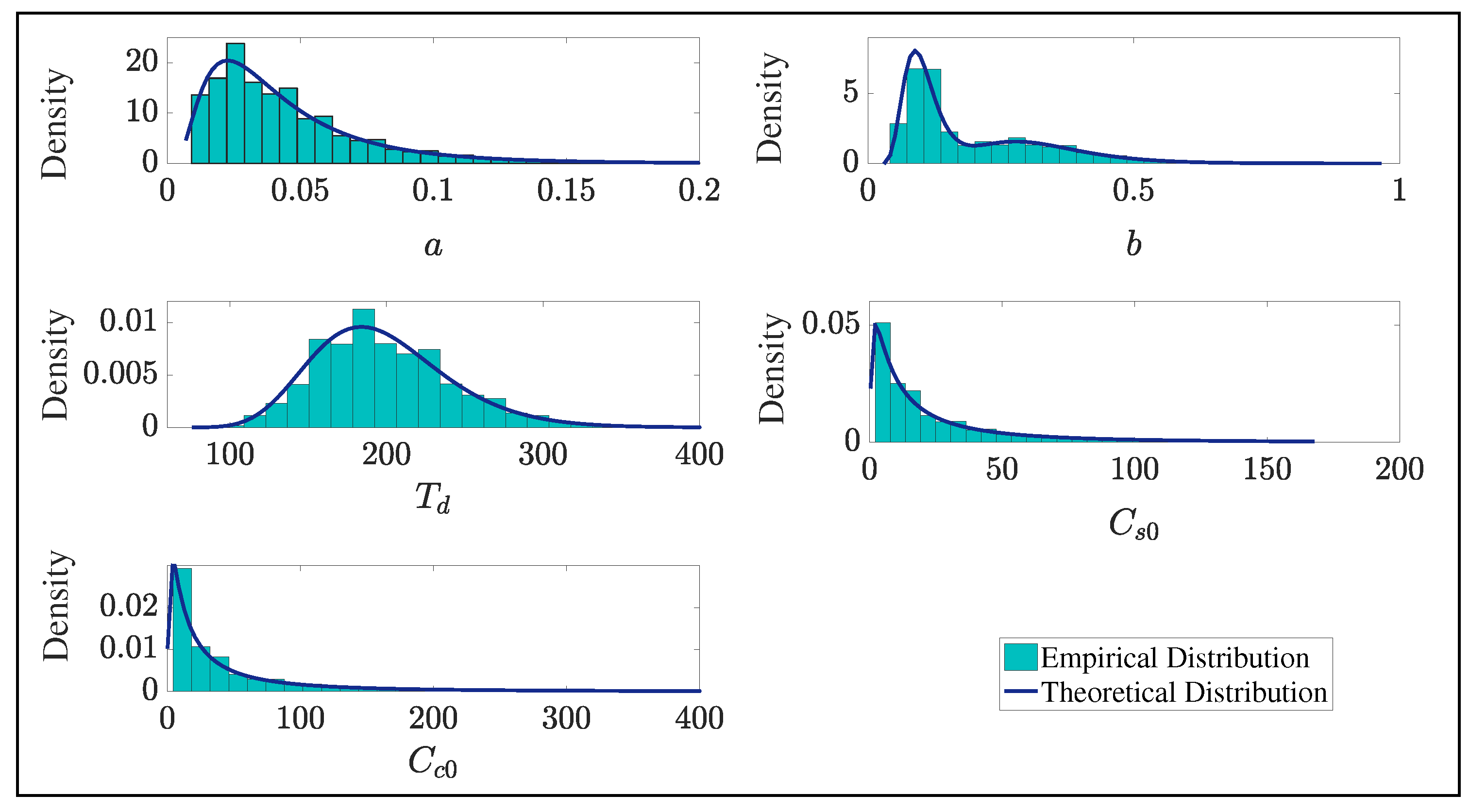
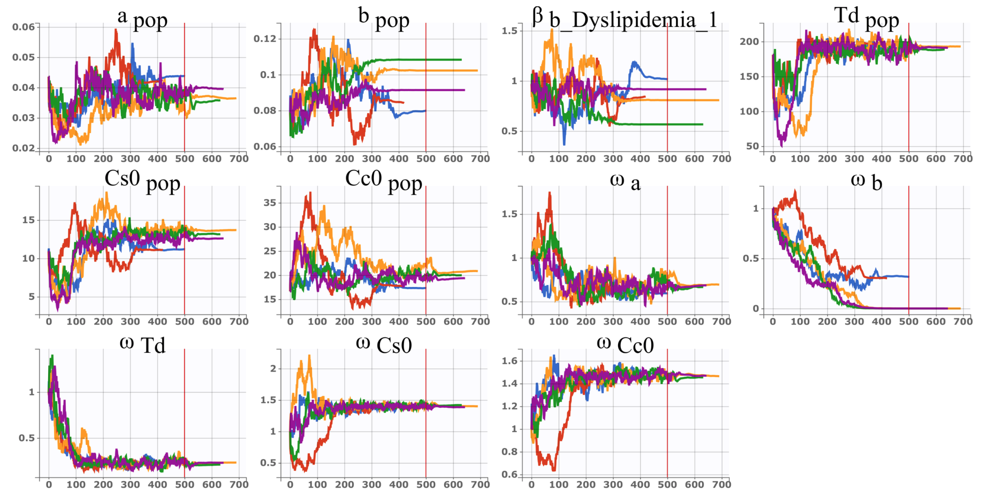
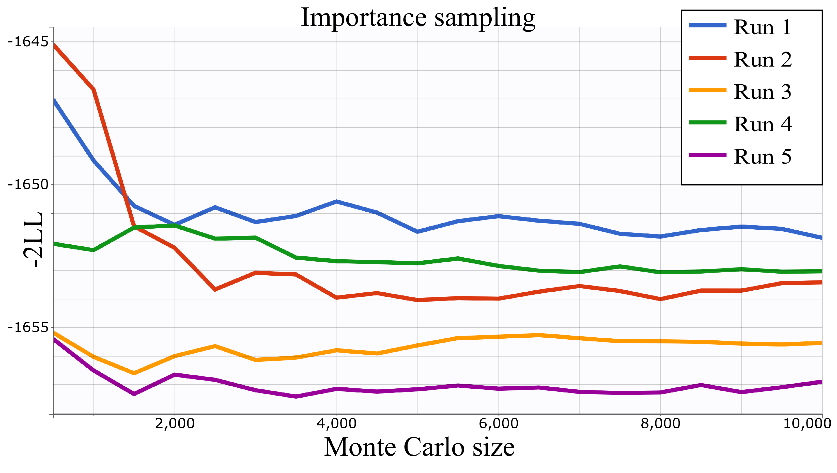
4.2. Parameter Estimation

The parameter estimation was performed by exploiting the SAEM algorithm. To ensure convergence towards a global optimum, an initial exploration phase was carried out using the simulated annealing algorithm: decreasing by 5% the variance of the random effects, and of the residual error parameter between two iterations, guarantees the exploration of a larger parameter space for a reasonable number of iterations. In such a manner, we can explore a larger space by improving the choice of the best starting point for subsequent parameter estimation [36]. The empirical and theoretical distributions of the obtained parameters estimate are reported in Figure 5 for all the parameters of model (6). All the empirical parameter distributions are nicely fitted through log-normal density functions, except for parameter b: in this case, the theoretical distribution exhibits a bimodal trend, which is interpolated by the mixture of two log-normal distributions (dyslipidemic and no-dyslipidemic groups). This bimodality was confirmed by means of Warren Sarle’s bimodality coefficient (BC), [40], which resulted as equal to 0.7.

Information about the estimated parameters is shown in

Table 3. Fixed and random effects estimated for each parameter. S.E. and R.S.E (%) are reported for both effects.

Fixed Effects
Parameter	Value	S.E.	R.S.E(%)
$a_{pop}$	0.0361	0.00675	18.7
$b_{pop}$	0.0986	0.0144	14.6
$\beta b_{Dyslip.}$	1.16	0.241	20.9
$T_{d_{pop}}$	193	17.9	9.26
$C_{s{0}_{pop}}$	15.1	4.3	28.4
$C_{c{0}_{pop}}$	23.5	7.34	31.2
Standard Deviation of the Random Effect
Parameter	Value	S.E.	R.S.E(%)
${\omega }_a$	0.682	0.165	24.2
${\omega }_b$	0.329	0.109	33.2
${\omega }_{T_d}$	0.221	0.0611	27.7
${\omega }_{C_{s0}}$	1.4	0.188	13.5
${\omega }_{C_{c0}}$	1.47	0.204	13.8

, which reports the typical value for the fixed effects, and the standard deviation of the random effects, explicable as the inter-individual variability. The standard error (SE) and the percentage relative standard error (RSE%) are quite limited, implying that the variability in the estimator remains low.

Such low variability in fixed- and random-effects coefficients, along with the good agreement between experimental measurements and model output (see Figure 6), let us conclude that the proposed mixed-effect model effectively describes the observed inter-individual variability in cTnT release. Figure 6 shows the results of the individual fitting for some patients: the reconstructed curves for every single patient are reported in comparison to the population model (red line). The results for all the 27 analyzed patients are shown in Figure S1 in the Supplementary Materials.

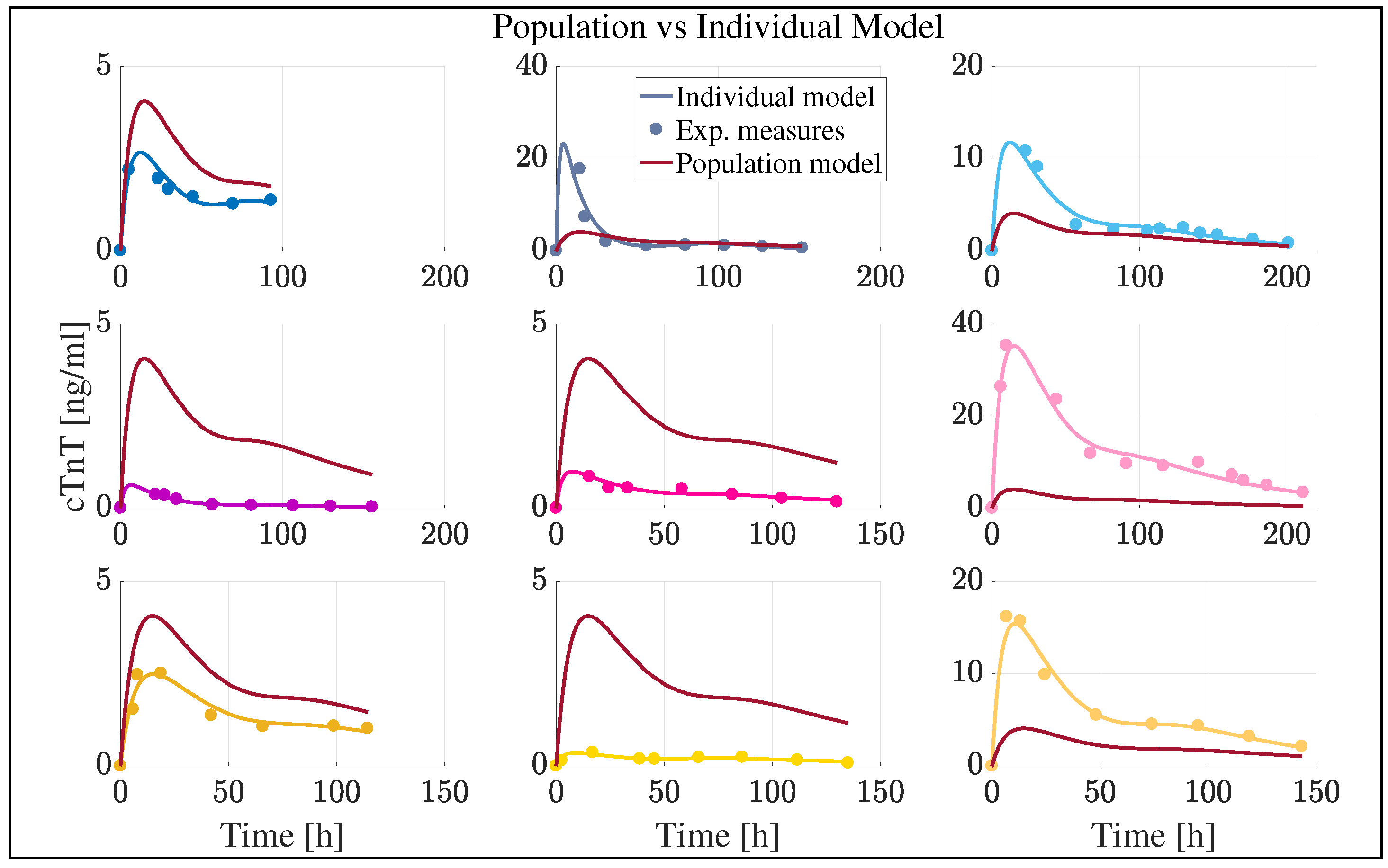
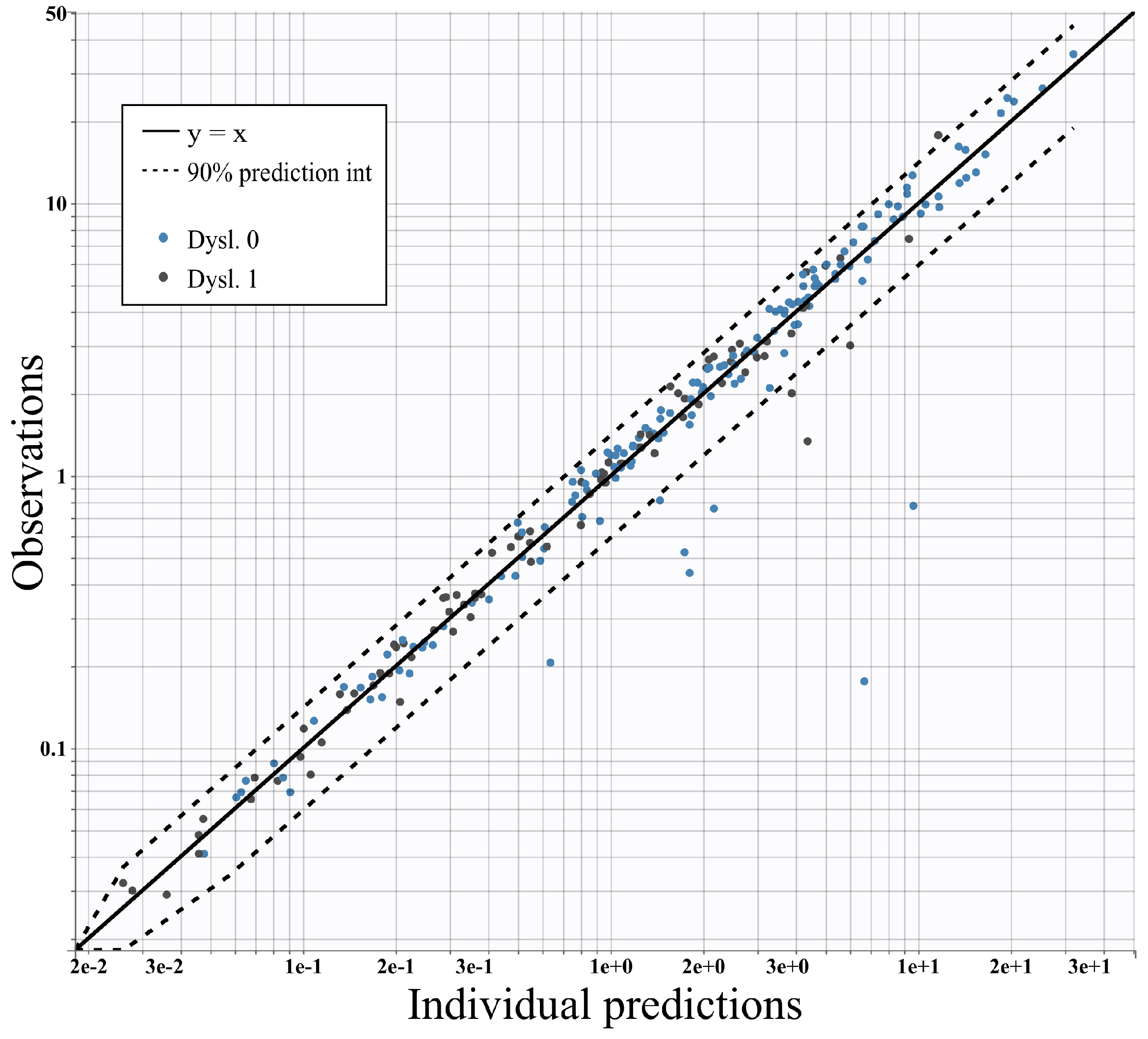
4.3. Assessment of the Model against Experimental Data

A visual predictive check analysis (VPC) was performed setting the number of the bins equal to 8: in this way, we achieved a good compromise between the approximation and estimation of the data. Furthermore, the least-squares criterion was chosen as the data-grouping method. Figure 7 shows the results of the VPC for the model of interest: the blue areas delimit the predicted percentiles for 10–90% while the red area represents 50% of the simulated dataset—here, we generate a dataset of 10,000 simulated time series.

The three blue lines indicate the empirical percentiles, while the red area and the red dots identify the areas outside the predicted intervals, and the outliers, as points located outside the closest percentile, respectively. From Figure 7, we can observe that the blue area for the 90 empirical percentile is very large, compared to the other ones: probably, this is due to the high variability in the observed data (blue dots). Furthermore, from Figure 7, it is possible to note that in the final part of the plot, the three quantiles appear closer than the model suggests. This means that in this part of the curve, the model could suggest incorrect results. A careful inspection of the results shown in Figure 7 reveals the presence of two outliers, distributed at the beginning and at the end of the curve: in particular, a small red area is localized in correspondence with the first outlier, probably due to the inconsistency in the first measurements, which is different for all the patients. Finally, to further assess the structural model, the relationship between observations and predictions was reported in Figure 8, where all the data are distributed among the line represented by the equation $y=x$. This suggests that the model is capable of correctly explaining all the experimental data. Note that the data outside the 90% prediction interval are associated with the first acquisition, as confirmation of the presence of the outlier and of the red area at the beginning of the curve in Figure 7.

However, no particular misspecification can be detected, confirming the suitability of the model. Figure 9 shows the results obtained from the convergence analysis of the MCMC method for five trajectories of the population parameters. This analysis consists of running the estimation task several times, starting from different randomly generated initial values of the fixed parameters. This type of test allows us to understand if MCMC has explored a parameter space large enough to reach the true posterior distribution of the parameters, and if the estimated values belong to that distribution [41].

As we can see from Figure 9, the results are in agreement in all five trajectories and, in particular, converge to roughly the same value of −2LL (i.e., the difference between two log likelihoods), as shown in Figure 10.

5. Discussion and Conclusions

In this paper, a novel approach based on an NME model was proposed for the analysis of cardiac-biomarkers release in AMI patients of the STEMI subclass. In particular, the inter-individual variability in the cTnT release time course was investigated, identifying the clinical covariates that have a significant influence on the parameters of the underlying release model. The proposed approach paves the way for the development of novel strategies to exploit cardiac-biomarkers acquisition in a clinical context, to gain patient-specific detailed valuable information for both diagnosis and prognosis.

From the preliminary analysis conducted in this work, despite the limited number of patients and the reduced number of considered covariates, we found a statistically significant relationship between dyslipidemia and the shape of the cTnT release curve. In particular, the results highlight its implications for the parameter related to the clearance of cTnT from the circulatory system. Further assessments of the proposed model concerned the evaluation of its ability to explain the experimental data by exploiting an MCMC strategy to sample the parameters model from a conditional distribution. Of note is that, despite the known clinical implication of dyslipidemia in cardiovascular disease, its direct influence on the cTnT release curve is not yet investigated in the literature. Notice that, despite the limited number of patients, the number of subjects with dyslipidemia in our dataset (9 out of 27) is coherent with the incidence rate encountered in AMI patients (20–40%). Furthermore, the statistical significance of the adjusted p value for the dyslipidemia covariate adds to the importance of our findings, providing a direction for future and more comprehensive investigation.

On the other hand, other covariates with a known clinical impact on cTnT levels, such as the presence of diabetes, do not show a statistically significant influence, according to the NME analysis, probably due to the limited number of subjects analyzed.

Another interesting finding is that dyslipidemic patients exhibit, on average, lower cTnT values with respect to non-dyslipidemic ones. This counter-intuitive finding, if confirmed in a larger cohort of patients, might be explained in several ways: one possibility is that it relates to the treatment with statins, a lipid-lowering drug, which exerts a protective function beyond their effect on blood cholesterol levels, by stabilizing the plaques and providing an anti-inflammatory effect.

Since age and gender represent two other important risk factors for AMI, [42], we proceeded to evaluate their impact on the dynamics of cTnT release: in relation to the experimental data of the analyzed population, and as reported in [43], their effects may be mainly on the basal level of cTnT in the systemic circulation, specifically in male patients of ages greater than 65 years. However, due to the characteristics of the analyzed population, these two factors did not show a significant impact on the release curve. Future analysis is planned of another clinically interesting model suggested by the analysis and reported in Table 1, i.e., model 3: this model suggests taking into account both dyslipidemia and age. In particular, from the analysis emerges that age could influence the parameter $T_d$, i.e., the threshold which allows modeling the release from sarcomere. Furthermore, a more thorough study on a larger dataset, including other potentially relevant covariates, e.g. renal failure (not available in the current dataset as none of the patients included had any impairment of renal function), and the circadian clock, will be the objective of our future work. Expanding the scope of our analysis, it will likely be possible to reveal other clinically relevant information that can be extracted from the cTnT release curve, including possible interactions between two or more covariates.

References

1. Tilea, I.; Varga, A.; Serban, R.C. Past, Present, and Future of Blood Biomarkers for the Diagnosis of Acute Myocardial Infarction—Promises and Challenges. Diagnostics 2021, 11, 881. [Google Scholar] [CrossRef] [PubMed]
2. Couch, L.S.; Sinha, A.; Navin, R.; Hunter, L.; Perera, D.; Marber, M.S.; Kaier, T.E. Rapid risk stratification of acute coronary syndrome: Adoption of an adapted European Society of Cardiology 0/1-hour troponin algorithm in a real-world setting. Eur. Heart J. Open 2022, 2, oeac048. [Google Scholar] [CrossRef] [PubMed]
3. Chaulin, A.M. Biology of Cardiac Troponins: Emphasis on Metabolism. Biology 2022, 11, 429. [Google Scholar] [CrossRef] [PubMed]
4. Bohn, M.K.; Higgins, V.; Kavsak, P.; Hoffman, B.; Adeli, K. High-sensitivity generation 5 cardiac troponin T sex-and age-specific 99th percentiles in the CALIPER cohort of healthy children and adolescents. Clin. Chem. 2019, 65, 589–591. [Google Scholar] [CrossRef] [PubMed] [Green Version]
5. Fournier, S.; Iten, L.; Marques-Vidal, P.; Boulat, O.; Bardy, D.; Beggah, A.; Calderara, R.; Morawiec, B.; Lauriers, N.; Monney, P.; et al. Circadian rhythm of blood cardiac troponin T concentration. Clin. Res. Cardiol. 2017, 106, 1026–1032. [Google Scholar] [CrossRef]
6. Lindstrom, M.J.; Bates, D.M. Newton–Raphson and EM algorithms for linear mixed-effects models for repeated-measures data. J. Am. Stat. Assoc. 1988, 83, 1014–1022. [Google Scholar]
7. Lindstrom, M.J.; Bates, D.M. Nonlinear mixed effects models for repeated measures data. Biometrics 1990, 46, 673–687. [Google Scholar] [CrossRef]
8. Montefusco, F.; Pedersen, M.G. Explicit theoretical analysis of how the rate of exocytosis depends on local control by Ca2+ channels. Comput. Math. Methods Med. 2018, 2018, 5721097. [Google Scholar] [CrossRef] [Green Version]
9. Sawlekar, R.; Montefusco, F.; Kulkarni, V.V.; Bates, D.G. Biomolecular implementation of a quasi sliding mode feedback controller based on DNA strand displacement reactions. In Proceedings of the 2015 37th Annual International Conference of the IEEE Engineering in Medicine and Biology Society (EMBC), Milan, Italy, 25–29 August 2015; pp. 949–952. [Google Scholar] [CrossRef]
10. Montefusco, F.; Procopio, A.; Bulai, I.M.; Amato, F.; Pedersen, M.G.; Cosentino, C. Interacting with COVID-19: How population behavior, feedback and memory shaped recurrent waves of the epidemic. IEEE Control. Syst. Lett. 2022, 7, 583–588. [Google Scholar] [CrossRef]
11. Parrotta, E.I.; Procopio, A.; Scalise, S.; Esposito, C.; Nicoletta, G.; Santamaria, G.; De Angelis, M.T.; Dorn, T.; Moretti, A.; Laugwitz, K.L.; et al. Deciphering the role of Wnt and Rho signaling pathway in iPSC-derived ARVC cardiomyocytes by in silico mathematical modeling. Int. J. Mol. Sci. 2021, 22, 2004. [Google Scholar] [CrossRef]
12. Davidian, M.; Gallant, A.R. The nonlinear mixed effects model with a smooth random effects density. Biometrika 1993, 80, 475–488. [Google Scholar] [CrossRef]
13. Aggrey, S. Logistic nonlinear mixed effects model for estimating growth parameters. Poult. Sci. 2009, 88, 276–280. [Google Scholar] [CrossRef]
14. Pinheiro, J.C.; Bates, D.M.; Lindstrom, M.J. Model Building for Nonlinear Mixed Effects Models; Department of Biostatistics Madison, University of Wisconsin: Madison, WI, USA, 1995. [Google Scholar]
15. Hickey, G.L.; Mokhles, M.M.; Chambers, D.J.; Kolamunnage-Dona, R. Statistical primer: Performing repeated-measures analysis. Interact. Cardiovasc. Thorac. Surg. 2018, 26, 539–544. [Google Scholar] [CrossRef] [Green Version]
16. Samson, A.; Lavielle, M.; Mentré, F. Extension of the SAEM algorithm to left-censored data in nonlinear mixed-effects model: Application to HIV dynamics model. Comput. Stat. Data Anal. 2006, 51, 1562–1574. [Google Scholar] [CrossRef] [Green Version]
17. French, R. Using Mixed Effects Modeling to Quantify Difference Between Patient Groups with Diabetic Foot Ulcers. Ph.D. Thesis, WKU Mahurin College, Bowling Green, KY, USA, 2017. [Google Scholar]
18. Ieva, F.; Paganoni, A.M.; Secchi, P. Mining administrative health databases for epidemiological purposes: A case study on acute myocardial infarctions diagnoses. In Advances in Theoretical and Applied Statistics; Springer: Berlin/Heidelberg, Germany, 2013; pp. 417–426. [Google Scholar]
19. Procopio, A.; De Rosa, S.; Covello, C.; Merola, A.; Sabatino, J.; De Luca, A.; Liebetrau, C.; Hamm, C.W.; Indolfi, C.; Amato, F.; et al. Estimation of the Acute Myocardial Infarction Onset Time Based on Time-Course Acquisitions. Ann. Biomed. Eng. 2021, 49, 477–486. [Google Scholar] [CrossRef]
20. Procopio, A.; Merola, A.; Cosentino, C.; De Rosa, S.; Canino, G.; Sabatino, J.; Ielapi, J.; Indolfi, C.; Amato, F. Analysis and classification of patients with acute myocardial infarction by using nonlinear mixed-effects modeling. In Proceedings of the 2021 IEEE 6th International Forum on Research and Technology for Society and Industry (RTSI), Virtual, 6–9 September 2021; pp. 569–573. [Google Scholar]
21. Ibanez, B.; James, S.; Agewall, S.; Antunes, M.J.; Bucciarelli-Ducci, C.; Bueno, H.; Caforio, A.L.; Crea, F.; Goudevenos, J.A.; Halvorsen, S.; et al. 2017 ESC Guidelines for the management of acute myocardial infarction in patients presenting with ST-segment elevation: The Task Force for the management of acute myocardial infarction in patients presenting with ST-segment elevation of the European Society of Cardiology (ESC). Eur. Heart J. 2018, 39, 119–177. [Google Scholar]
22. Roffi, M.; Patrono, C.; Collet, J.P.; Mueller, C.; Valgimigli, M.; Andreotti, F.; Bax, J.J.; Borger, M.A.; Brotons, C.; Chew, D.P.; et al. 2015 ESC Guidelines for the management of acute coronary syndromes in patients presenting without persistent ST-segment elevation: Task Force for the Management of Acute Coronary Syndromes in Patients Presenting without Persistent ST-Segment Elevation of the European Society of Cardiology (ESC). Eur. Heart J. 2016, 37, 267–315. [Google Scholar]
23. Mair, J.; Artner-Dworzak, E.; Lechleitner, P.; Smidt, J.; Wagner, I.; Dienstl, F.; Puschendorf, B. Cardiac troponin T in diagnosis of acute myocardial infarction. Clin. Chem. 1991, 37, 845–852. [Google Scholar] [CrossRef]
24. Wu, A.H. Release of cardiac troponin from healthy and damaged myocardium. Front. Lab. Med. 2017, 1, 144–150. [Google Scholar] [CrossRef]
25. Lavielle, M.; Mentré, F. Estimation of population pharmacokinetic parameters of saquinavir in HIV patients with the MONOLIX software. J. Pharmacokinet. Pharmacodyn. 2007, 34, 229–249. [Google Scholar] [CrossRef] [Green Version]
26. Moon, T.K. The expectation-maximization algorithm. IEEE Signal Process. Mag. 1996, 13, 47–60. [Google Scholar] [CrossRef]
27. Delyon, B.; Lavielle, M.; Moulines, E. Convergence of a stochastic approximation version of the EM algorithm. Ann. Stat. 1999, 27, 94–128. [Google Scholar] [CrossRef]
28. Bergstrand, M.; Hooker, A.C.; Wallin, J.E.; Karlsson, M.O. Prediction-corrected visual predictive checks for diagnosing nonlinear mixed-effects models. AAPS J. 2011, 13, 143–151. [Google Scholar] [CrossRef] [PubMed] [Green Version]
29. Procopio, A.; De Rosa, S.; Covello, C.; Merola, A.; Sabatino, J.; De Luca, A.; Indolfi, C.; Amato, F.; Cosentino, C. Mathematical model of the release of the CTNT and CK-MB cardiac biomarkers in patients with acute myocardial infarction. In Proceedings of the 18th European Control Conference, Naples, Italy, 25–28 June 2019; pp. 1653–1658. [Google Scholar]
30. Procopio, A.; De Rosa, S.; García, M.R.; Covello, C.; Merola, A.; Sabatino, J.; De Luca, A.; Indolfi, C.; Amato, F.; Cosentino, C. Experimental Modeling and Identification of Cardiac Biomarkers Release in Acute Myocardial Infarction. IEEE Trans. Control. Syst. Technol. 2020, 28, 183–195. [Google Scholar] [CrossRef]
31. Procopio, A.; De Rosa, S.; Montefusco, F.; Canino, G.; Merola, A.; Sabatino, J.; Ielapi, J.; Indolfi, C.; Amato, F.; Cosentino, C. CBRA: Cardiac biomarkers release analyzer. Comput. Methods Programs Biomed. 2021, 204, 106037. [Google Scholar] [CrossRef]
32. Crank, J. The Mathematics of Diffusion; Oxford University Press: Oxford, UK, 1979. [Google Scholar]
33. Procopio, A.; Bilotta, M.; Merola, A.; Amato, F.; Cosentino, C.; De Rosa, S.; Covello, C.; Sabatino, J.; De Luca, A.; Indolfi, C. Predictive mathematical model of cardiac troponin release following acute myocardial infarction. In Proceedings of the 2017 IEEE 14th International Conference on Networking, Sensing and Control (ICNSC), Calabria, Italy, 16–18 May 2017; pp. 643–648. [Google Scholar]
34. Villaverde, A.F.; Barreiro, A.; Papachristodoulou, A. Structural Identifiability of Dynamic Systems Biology Models. PLoS Comput. Biol. 2016, 12, e1005153. [Google Scholar] [CrossRef] [Green Version]
35. Villaverde, A.F. Observability and Structural Identifiability of Nonlinear Biological Systems. Complexity 2019, 2019, 8497093. [Google Scholar] [CrossRef] [Green Version]
36. Chan, P.L.; Jacqmin, P.; Lavielle, M.; McFadyen, L.; Weatherley, B. The use of the SAEM algorithm in MONOLIX software for estimation of population pharmacokinetic-pharmacodynamic-viral dynamics parameters of maraviroc in asymptomatic HIV subjects. J. Pharmacokinet. Pharmacodyn. 2011, 38, 41–61. [Google Scholar] [CrossRef] [Green Version]
37. Morrow, D.A.; Antman, E.M.; Charlesworth, A.; Cairns, R.; Murphy, S.A.; de Lemos, J.A.; Giugliano, R.P.; McCabe, C.H.; Braunwald, E. TIMI risk score for ST-elevation myocardial infarction: A convenient, bedside, clinical score for risk assessment at presentation: An intravenous nPA for treatment of infarcting myocardium early II trial substudy. Circulation 2000, 102, 2031–2037. [Google Scholar] [CrossRef] [Green Version]
38. Muller, J.E.; Stone, P.H.; Turi, Z.G.; Rutherford, J.D.; Czeisler, C.A.; Parker, C.; Poole, W.K.; Passamani, E.; Roberts, R.; Robertson, T.; et al. Circadian variation in the frequency of onset of acute myocardial infarction. N. Engl. J. Med. 1985, 313, 1315–1322. [Google Scholar] [CrossRef]
39. Takeda, N.; Maemura, K. Circadian clock and cardiovascular disease. J. Cardiol. 2011, 57, 249–256. [Google Scholar] [CrossRef] [Green Version]
40. Knapp, T.R. Bimodality revisited. J. Mod. Appl. Stat. Methods 2007, 6, 3. [Google Scholar] [CrossRef]
41. Nylander, J.A.; Wilgenbusch, J.C.; Warren, D.L.; Swofford, D.L. AWTY (are we there yet?): A system for graphical exploration of MCMC convergence in Bayesian phylogenetics. Bioinformatics 2008, 24, 581–583. [Google Scholar] [CrossRef] [Green Version]
42. Mueller, M.; Vafaie, M.; Biener, M.; Giannitsis, E.; Katus, H.A. Cardiac Troponin T–From Diagnosis of Myocardial Infarction to Cardiovascular Risk Prediction. Circ. J. 2013, 77, 1653–1661. [Google Scholar] [CrossRef] [Green Version]
43. Gore, M.O.; Seliger, S.L.; Defilippi, C.R.; Nambi, V.; Christenson, R.H.; Hashim, I.A.; Hoogeveen, R.C.; Ayers, C.R.; Sun, W.; McGuire, D.K.; et al. Age-and sex-dependent upper reference limits for the high-sensitivity cardiac troponin T assay. J. Am. Coll. Cardiol. 2014, 63, 1441–1448. [Google Scholar] [CrossRef]
Figure 1. (i) Cardiac troponin complex is composed of three different protein subunits, each of which has a specific role in cardiac contraction: (1) subunit C, designed to bind the C a 2 + , (2) subunit I, binds to actin in thin myofilaments, and (3) subunit T, connected to tropomyosin. (ii) In a typical healthy cardiomyocyte, all the fibers appear intact, and none of the three cardiac troponin subunits is appreciably detectable in the systemic circulation. (iii) During an AMI, the myocardial tissue downstream of the vascular obstruction goes into necrosis: the myofibers disintegrate and the cellular membrane breaks down, allowing components of the troponin complex to reach the circulatory system. Several abnormalities can be observed on ECG tracings. Among them, an elevation in the ST segment, especially during the initial phase of an AMI, is associated with a larger clinical risk, suggesting complete coronary obstruction. This type of AMI is called STEMI (ST-elevation myocardial infarction) and requires prioritized management, being associated with a higher risk for mortality and clinical complications, especially in the absence of timely restoration of blood flow to the infarcted area.
Applsci 12 13038 g001
Figure 2. Graphical representation of the stochastic approximation version of the expectation-maximization algorithm (SAEM) in combination with the MCMC method. To ensure the global optimization solution, SAEM proceeds through two distinct steps: (i) the exploratory phase, during which the entire parameter space is explored, and (ii) the smoothing phase, during which the optimal solution is refined.
Applsci 12 13038 g002
Figure 3. Distribution of all the available categorical and continuous covariates among the 27 STEMI patients of the study. Note that covariates such as ejection fraction, hemoglobin, and anterior wall are not included in the analysis.
Applsci 12 13038 g003
Figure 4. Time course of the concentration levels of cTnT into the plasma of the 27 STEMI patients, with and without dyslipidemia. Each color is associated with the time series of a different patient.
Applsci 12 13038 g004
Figure 5. Empirical and theoretical distribution of the estimated values for each parameter of the model (6). The distribution for parameter b clearly exhibits a bimodal trend, confirmed by evaluating Warren Sarle’s bimodality coefficient (BC) which for the distribution of the estimated values for parameter b is >0.5 (0.7).
Applsci 12 13038 g005
Figure 6. Model results for some of the 27 STEMI patients. For each subject, the population model (red light line), obtained by the fixed effects estimated from all the patients, and the individual fit (colorful line), obtained by taking into account the random effects, are reported. The experimental acquisitions are denoted by dots.
Applsci 12 13038 g006
Figure 7. Visual predictive check analysis computed on the whole population, and obtained by simulating, through the Monte-Carlo method; 10,000 time series.
Applsci 12 13038 g007
Figure 8. Observations vs individual predictions for the model taking into account the dyslipidemic covariate (i.e., model 2 in Table 1).
Applsci 12 13038 g008
Figure 9. Population parameter estimates with respect to the iterations of SAEM during the convergence assessment of the model. Each color refers to a trajectory.
Applsci 12 13038 g009
Figure 10. Distribution of the −2LL values for each iteration among all the five trajectors.
Applsci 12 13038 g010