Leveraging Machine Learning and Semi-Structured Information to Identify Political Views from Social Media Posts

Abstract

Social media platforms make a significant contribution to modeling and influencing people’s opinions and decisions, including political views and orientation. Analyzing social media content can reveal trends and key triggers that will influence society. This paper presents an exhaustive analysis of the performance generated by various implementations of the Naïve Bayes classifier, combined with a semi-structured information approach, to identify the political orientation of Twitter users, based on their posts. As research methodology, we aggregate in a semi-structured format a database of over 86,000 political posts from Democrat (right) and Republican (left) ideologies. Such an approach allows us to associate a Democrat or Republican label to each tweet, in order to create and train the model. The semi-structured input data are processed using several NLP techniques and then the model is trained to classify the political orientation based on semantic criteria and semi-structured information. This paper examines several variations of the Naïve Bayes classifier suite: Gaussian Naïve Bayes, Multinomial Naïve Bayes, Calibrated Naïve Bayes algorithms, and tracks a variety of performance indices and their graphical representations: Prediction Accuracy, Precision, Recall, Confusion Matrix, Brier Score Loss, etc. We obtained an accuracy of around 80–85% in identifying the political orientation of the users. This leads us to the conclusion that this type of application can be integrated into a more complex system and can help in determining political trends or election results.

1. Introduction

Social media platforms are now present in our daily lives and have made a significant contribution to modeling and influencing people’s opinions and decisions. The analysis of the content we post on social media platforms can facilitate the identification and analysis of opinions, ideas, and trends among users, including political orientation and preferences. The content of our posts in our online presence reveals a lot about the personality of users and their opinions [1]. Moreover, analyzing social media content can reveal trends and key triggers that will influence society.

Among social media platforms, Twitter generates large amounts of text containing political insights, which can be analyzed to extract the users’ opinions and predict trends in elections. Our research uses semi-structured information as input data and various forms of the Naïve Bayes classifier to examine the identification of political orientation of Twitter users, based on the content of their posts, in terms of Democrat and Republican classification. The second objective is to calculate performance metrics related to several machine learning models and algorithms in order to make a comparison of their accuracy on the proposed data set. As practical usability, the application can be used in real case scenarios to predict the election results, to monitor and evaluate the evolution of political preferences of social media users, to establish if a politician or political party increases or decreases in popularity, and even to predict the dynamics of political movements.

The choice of tweet posts as input was inspired by the candidacy of US President Donald Trump. During his mandate, he accelerated an already existing trend in the online environment, namely posting personal opinions on Twitter, related to various events, laws, news, etc., in an informal manner, very close to the natural language used in daily life. Many other political leaders followed his model and posted more actively on the social network Twitter, the platform also gaining over six million new users in the first quarter of 2018 [2]. This phenomenon is called “The Trump Effect”.

The context presented above has the classic structure of a Topic Classifying issue, in which machine learning models must frame the input data in a certain class according to common features. More precisely, the classification is made according to the words mainly used in the posts of Democrats and Republicans. The ideologies of the two political orientations are linked to different points of view related to highly popular topics, such as abortion, gun ownership, racism, army development, the death penalty, and emigration [3].

As research methodology, we aggregated in a semi-structured format (CSV) a database of over 86,000 political posts related to the topics mentioned above. Such an approach allows us to associate a Democrat or Republican label to each tweet. By analyzing the content of tweets and verifying the labels, the AI model will learn to tag tweets on its own, in a supervised learning process. This paper examines several variations of the Naïve Bayes classifier suite: Gaussian Naïve Bayes, Multinomial Naïve Bayes, Calibrated Naïve Bayes algorithms, and tracks a variety of performance indices and their graphical representations: Prediction Accuracy, Precision, Recall, Confusion Matrix, Brier Score Loss, etc. The implementation is carried out in Python, known as the main programming language, used in the AI field.

2. Related Work

Social media is increasing in popularity at a very fast pace, and so is the number of users, which leads to huge amounts of unstructured text posted on these platforms. Besides exchanging information, users on social media also express their ideas and opinions about different topics, such as products, travel, food, and even politics and people. Consequently, users express their sentiments about people, organizations, places, or ideas. Among them, Twitter is a social media platform which generates large amounts of text containing political insights, which can be analyzed to extract the users’ opinions and predict trends in the elections.

Social networks have the potential to revolutionize the world of social science research, or Social Science Engineering [4]. Twitter is mainly used by specialists because of its text-oriented content. The popularity of the Twitter platform is growing both socially and scientifically, and its content is used in more and more varied research.

In addition to using tweets for Topic Classifying applications, they are very popular as a research resource for Sentiment Analysis. This topic is related to extracting the positive or negative perception from a text document, and according to [5], tweet posts were used because it was concluded that the analysis on shorter and concise texts is more efficient and offers better performance. This type of analysis is often found in services such as movie recommendations, products, reviews, ranking, and sorting by preferences.

In [6], a framework that aggregated user interactions on social for demographics and personality discovery tasks was proposed. The authors of [7] developed a study in which customers reacted to a retailer’s political opinion posted on a social media account.

In addition, according to [8], in the field of natural language processing, research studies are conducted on emoticons and hashtags used in tweets, as these elements also provide significant informational load for the content. The paper concludes that using the correct hashtags in a tweet post already frames that post in a certain class, and links it to a certain trend.

In [9], the textual analysis of the data on Twitter is made based on full-text, hashtags, and data clusters and the purpose of the paper is to classify tweets according to the Democrat and Republican political orientation of the users. The use of neural networks as a prediction mechanism in the aforementioned paper leads to better performance indices than in the case of probabilistic algorithms, resulting in a final prediction accuracy of about 94%.

An intelligent threatening language detection that uses machine learning and deep learning models is described in [10]. The authors of [11] developed a deep learning-based system used for information triaging on Twitter during several situations, such as emergency situations or influential events. Perez-Landa et al. [12] classified the posts on Twitter using a natural language processing approach and an explainable artificial intelligence model.

Baute presented the study of transcripts in the parliamentary debates in the United States of America. Using only the written form of politicians’ natural language as input data, the study investigates a politician’s agreement or disagreement on a political proposal, depending on the words he or she uses to express his or her opinion. Of course, on average, the agreement or disagreement of a political representative on a respective political proposal was in line with the ideologies of the party to which he belonged. This is, in fact, also a verification step in the context of NLP.

In [13], the authors proposed a methodology to predict the outcome of election results by utilizing the user influence factor, using a combined approach between Principal Component Analysis and SVM.

This research examines the performance of various forms of the Naïve Bayes algorithm in detecting the political orientation (Democrat and Republican), based on tweets.

3. The Methodology Used for the Implementation

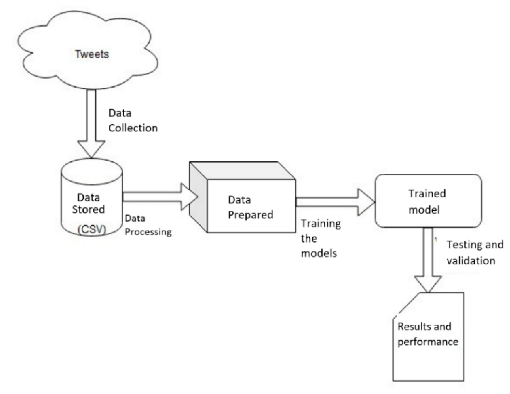
This section presents the implementation of the system and the steps undertaken in order to achieve the goals of the research, namely the identification of an individual’s political orientations based on their tweets, as well as the analysis of results obtained using various NLP algorithms and models. The proposed research is based on 2 main phases:

• Data preparation: aggregating a set of tweets in a CSV document—semi-structured format, using NLP techniques, such as tokenization, lemmatization, eliminating stop-words
• Training ML models on the prepared data, using several Naïve Bayes algorithm versions in order to conduct a comparative analysis of the performance

Figure 1 illustrates the main steps undertaken in the implementation and validation process.

We used Scikit-learn, a Python library for machine learning to build a classifier in Python. The steps to build a classifier in Python are as follows:

• Import the Sklearn Python package.
• Import the data set, in order to build the classification prediction model.
• Organize the input data into two sets: one training data set and one test data set. We use the train_test_split function of the Sklearn python package to split the data into sets.
• Create and evaluate the model: After splitting the data into training and testing sets, we will create the model for identifying political orientation and evaluate it. For this purpose, we use the Naïve Bayes suite of algorithms to create several models and evaluate their performance. For evaluation purposes, we use the predict function to make predictions.
• Calculate performance indicators to evaluate performance.

3.1. Data Collection

The input data used for this research are the tweet posts of some political personalities whose political orientation is known. The data set used consists of 3 aggregated open source data sets available on the Kaggle platform. This data set was used to train the model. As a large number of such posts is needed in order to carry out the training process and obtain quality results, 86,460 political posts were aggregated as input data and stored in semi-structured format (CSV). Initially, 100,000 posts were retrieved, but some of the tweets were omitted due to the fact that they did not meet the requirements and did not contribute to the training of the model. The final collection of tweets, however, meets the performance requirements and also allows the data set to be divided into training, testing and validation sets. To train the models, the tweets were labeled Democratic (left), respectively, Republican (right). In order to facilitate the computational process, the value 1 was assigned for the Democratic label, namely the value 0 for the Republican label.

An example of a Democrat tweet is: “We need to transition to low carbon economy”, posted by House Agriculture Committee Chairman David Scott, while a Republican tweet is: ”More than 80% of Americans support requiring work-capable adults to participate in a job or training program at least.”, posted by Steve Scalise, United States House of Representatives.

The data were collected through the Twitter API [14], which provides access to data and metadata. Additionally, a software tool called Hydrator [15] was used to automate the process of obtaining posts from the Twitter platform and store them in a semi-structured format. This tool is available in open-source format on Github. The result was a CSV file with 86,460 entries arranged in two columns: Tweet (post content) and Party (political party). These data were then extracted using the Python module, Pandas [16], and entered into a DataFrame object, as can be seen in Figure 2:

In order not to affect the performance of the model and to have a balanced data set, the Democratic and Republican tweets were divided in almost equal sets. Thus, as a percentage, we have 49% Democratic tweets and 51% Republican tweets (Figure 3). Numerically, there are 44,095 posts labeled as Republican and 42,365 Democratic posts.

Thus, at this point, the data set are aggregated, well distributed, labeled and prepared for the next stage of data processing using NLP techniques.

3.2. Input Data Processing

The input data collected in the first step are processed using a set of fundamental and acknowledged techniques for the NLP domain [17].

• The first procedure applied on the data is the elimination of punctuation. Given that tweet posts are close to natural language, they do not follow spelling and punctuation rules. In general, abbreviations are used in a tweet, punctuation marks are non-existent, too few, or used incorrectly. The case where a post follows all the grammatical norms is rare, even if some posts come from some great political individuals. Therefore, to perform this procedure we use a regular expression, or RegEx.
• Transform all characters in lower-case, using a predefined Python method. This plays an important role in the characteristics matrix which is used in training the models.
• The next steps in the data processing are the tokenization, lemmatization, and stemming processes, implemented through the Natural Language Toolkit (NLTK) platform [18]. Tokenization splits the text based on separators, the most commonly used being the space to generate the most common type of token—the word. This is also the approach used in this research. Once we obtained the tokens, we applied the lemmatization and stemming procedures. Lemmatization groups the different inflected forms of a word, so that they are further treated as a single element. Bringing the words to the basic form takes into account several forms of derivation, such as the plural, conjugation according to person or tense, possessive pronouns, datives, and superlative forms. Stemming removes or replaces word suffixes to reduce words to their common root. Lemmatization and stemming are quite similar; however, lemmatizing focuses more on the context of words and on their morphological analysis [19].

Thus, the tokenized text is further processed, and the vocabulary initially obtained is substantially reduced by merging tokens that refer to the same element.

4.

Remove Stop Words—connection terms connection, conjunctions, interjections, indefinite article, etc., will be removed. The purpose of this step is to isolate only the terms with high informational value. We used the specialized utility from the NLTK package, which automates the process of removing Stop-Words. Lists of such keywords have been built over time but are constantly updated. Using the NLTK utility which we finally obtained, after all the procedures performed in this subsection, the set of posts were prepared for the next stage.

In order to observe the differences before and after processing, let us analyze as an example the content of the following unprocessed Republican post: “#Zika fears realized in Florida. House GOP acted to prevent the crisis. Dems in action, inexcusable! Time to put politics aside & work together!”. After all the processing techniques mentioned above have been applied, this tweet becomes: “zika fear realize Florida House GOP act prevent crisis Democrat action in excuse time put political aside work together”. It can be noticed how unknown tokens such as “zika” or “gop” were kept, and the rest of the terms were brought back to basic form. These applied procedures make the classification of posts much easier. Now, even an analysis performed with the naked eye on the keywords in this post can already direct us to the political ideology of the individual who posted this tweet. Further on, we automate this process with the help of the algorithms which is presented in Section 4.

3.3. Input Data Analysis

After the word processing procedures described in the previous subchapter, we obtained the data set prepared for analysis. To perform a more detailed analysis of the data before using to train the models, we used the Wordnet [20] utility in the NLTK package. Specifically, Wordnet was created by Princeton to be able to give meaning, definitions, synonyms, and antonyms to words. Thus, we used Wordnet to mark the synonyms in our data set. This analysis of the meaning of words reduces the number of different terms in the feature matrix and helps analyze the degree of informational load of each term used in model training. The resulting data set was further transformed with a Vectorizer Count [21], which converts a collection of texts to a matrix of token counts and placed in the final form. It was used to further train the models based on it.

The Bag-of-Words principle [22] is first used, where we extract the main features from the text document with processed posts. This principle is used to emphasize the degree of appearance of words, which means that we are more interested in the occurrence of the terms in the document and not their position. In order to be able to use the most used words as features in the model training, we create an array of such characteristics. The elements of the feature matrix must be clear and concise, as the use of ambiguous features in the training process is not recommended.

Because the number of terms obtained for the feature set is very large, a compromise must be made so that we only use terms that carry a strong information load. Therefore, in the matrix mentioned above we aggregate the 5000 most used terms. In order to test the ratio between resources and processing time, we tried to run with 6000 and 7000 such terms, respectively, but the performance was poorly improved, resulting in the fact that the remaining added terms did not bring much information in decision making under the algorithm classification.

Figure 4 shows the occurrence distribution of the first 10 political terms in our data set, which helps in the features analysis for the training of the models.

Further analyzing the rest of the terms, we notice their political and legislative nature. In addition, there are notorious terms debated by the two political orientations, usually in opposition, such as war/peace and debt/prosperity. Besides the political and legislative words, terms such as irresponsible, unacceptable, excuses, and immorality also stand out in the data set.

Figure 5 depicts the number of occurrences of the selected terms, in correlation with Figure 4.

The initial data set with the 86,000 tweets that was processed, resulting in the matrix of terms analyzed in this subchapter, are further divided into smaller sets, used for training, testing, and validation. First, 80% of the input data are used to train the models. Afterwards, the next step is to run a test using 90% of the data set, to compare performance.

4. Machine Learning Algorithms and Models

This section is dedicated to choosing, implementing, and training the models based on ML algorithms. Considering the objectives of our research, the identification of the political orientation based on Twitter posts, we chose three variations of the Naïve Bayes algorithm: Gaussian NB, Multinomial NB, Bernoulli NB, and performed a comparative analysis of their performance.

4.1. The Naïve Bayes Algorithm

The Naïve Bayes algorithm is based on Bayes’ theorem [23], based on conditional probabilities of events. The initial conditioning of the algorithm introduces the hypothesis that there is no correlation between the predictors used in the feature matrix. Thus, these features independently contribute to the decisions made by the algorithm.

Given a vector of characteristics x = [x1, x2,…, xn], respectively the class of labels c ∈ {1, 2,…, C}, the probability of a given event of features to belong to a class is [24] (Figure 6):

The NB classifier is defined as [25]:

$$\widehat{y}=arg\underset{c\in 1,\dots ,\complement }{\underbrace{max} }p\left(c\right){\displaystyle \prod }_{i=1}^{n}p(x_i|c)$$

(1)

As the previous values of the probabilities p(x_i|c) are calculated and learned during the training process, the contributions of each element of the features matrix can be calculated based on the previously calculated values: p(c|x_i) = p(c) p(x_i|c)/p(x_i). This calculation method is called prior probability computation [24].

The Naïve Bayes algorithm is one of the most well-known supervised learning classifiers, highly used in NLP [26]. The algorithm is specialized in class classification, namely, it is used to analyze text data and classify it into categories—categorical text data.

The major difference between the Multinomial NB algorithm and the standard Naïve Bayes variant is found in the distribution of probabilistic data. Specifically, in the case of Multinomial NB, the probabilities p(f_i|c) (the conditional probability of a feature f given the class c) have a multinomial distribution. Based on this type of distribution, the algorithm handles data well that can be classified according to occurrence, such as the appearance of certain terms in a text.

Multinomial distribution is based on repeated events, such as rolling a dice several times, and it is a type of discrete probability distribution. In this case, we can map the probability of each event to occur to their number of occurrences in the tests performed. Multinomial distribution is a generalization of binomial distribution. The basic formula of a multinomial probability distribution is as follows [25]:

$$P\left(x\right)=\frac{n!}{x_1! · x_2! · \dots · x_k!} · p_1{}^{X_1}· p_2{}^{X_2}·\dots · p_k{}^{X_k}$$

(2)

where $X_1+X_2+\dots +X_k=n$ and $p_1+p_2+\dots +p_k=1$, $X_i$ is the occurance of event $E_i$, and $p_i$ id the probability of event $E_i$.

4.2. The Gaussian Naïve Bayes Algorithm

The Gaussian Naïve Bayes algorithm is a variant of Naïve Bayes based on Gaussian/normal distribution, which supports continuous data [26]. The Gaussian NB algorithm also calculates the mean and standard deviation of the data in addition to the basic calculations related to probabilities according to the Bayes theorem. The mean can be calculated using the formula:

$$mean\left(x\right)=\frac{1}{n}·sum\left(x\right)$$

(3)

The standard deviation can be calculated for each input variable with the formula:

$$std\left(x\right)=\sqrt{\frac{1}{n} ·sum(x_i-mean{\left(x\right)}^2 }$$

(4)

For the calculation of the probabilities of the new values the Gaussian density formula is used, PDF—Gaussian Probability Density Function. It is based on the above formulas for mean and standard deviation:

$$pdf\left(x, mean, std\right)=\frac{1}{\sqrt{2\pi }·std}· e^{-\frac{x-mea{n}^2}{2 · st{d}^2}}$$

(5)

4.3. The Bernoulli Naïve Bayes Algorithm

While the classifiers presented in the previous sections measure the occurrence of some features in the model, the Bernoulli NB algorithm [23] determines the presence or absence of a certain feature in a text, based on discrete probabilities.

The main property of the Bernoulli NB algorithm is that it works with binary features. Thus, it analyzes the probability that a document will be found in a certain class, considering whether or not certain features are found in that text document. For a feature vector $x_i$ and a set of classes c, the Bernoulli algorithm is based on the following formula:

$$P\left(x_i|c\right)=P\left(i|c\right)x_i+\left(1-P\left(i|c\right)\right)\left(1-x_i\right)$$

(6)

Within the Bernoulli distribution, for each experiment that can be completed either successfully or with failure, a probability p is assigned for the event to end successfully, namely a probability q = 1 − p, for it to end with failure.

4.4. The Calibrated Naïve Bayes Algorithm

Calibration is used when the distribution on which the algorithm is based is not exactly suitable for the data set to be classified [23]. Thus, if we consider a data set that cannot be completely modeled with a certain distribution, we can calibrate the algorithm in the implementation stage [21].

The calibration of a classifier is carried out using a regressor, called a calibrator, which maps the output of the classifier to a calibrated probability value. There are two types of calibrators: sigmoid and isotonic [27].

The sigmoid calibrator, also called Platt Scaling, is based on a logistic regression according to the formula below, in which f(x) represents a logistic transformation of the classifier, and A and B are two scalar parameters estimated using the maximum likelihood method.

$$P \left(y=1|x\right)=\frac{1}{1+\exp \left(A f\left(x\right)+B\right)}$$

(7)

The isotonic calibrator, also called monotonic, is based on minimizing the argument of an isotonic regression function. The isotonic regression problem we start from is given by the following equation, where m is the isotonic function:

$$y_i=m \left(f_i\right)+{ϵ}_i$$

(8)

Both sigmoid and isotonic calibration will be used in this research.

For the implementation of these algorithms, we used the Sklearn library (Scikit-learn) [26], which is a powerful tool when it comes to developing ML applications in Python. This library provides algorithms for model training, processing, and evaluation utilities, as well as estimation methods. In Sklearn, an estimator is an object with which a model is built based on input data (drive data) and which performs calculations that correspond to the properties, in order to obtain a result for a new, unknown data set (test data). In other words, an estimator can be a regressor or a classifier. All estimators inherit the basic class sklearn.base.BaseEstimator with its methods and properties.

5. Results and Discussion

This section is dedicated to the presentation and analysis of the results obtained. Different metrics and techniques for measuring and analyzing the aforementioned performances are used: Prediction Accuracy, Precision, Recall, Confusion Matrix, and Brier Score Loss.

Let us first analyze the data used for the training and testing phases. The data set was divided using the Train Test-Split functionality [27] from the Sklearn library to test the performances with 80–20, respectively, 90–10 ratios for the training data, respectively, test data. The test_size parameter set to 0.2 will generate the first mentioned ratio, and the value 0.1, will generate the second ratio. Train vectors and test vectors are further used in training and prediction analysis. Following the training process, the prediction method is used to obtain the classification of the data in the two categories, which we then analyze the obtained labels. For the data set of 86,460 posts, when using a 90–10 data split ratio, there are 8646 in the test data, while using an 80–20 ratio, there are 17,292 entries as test data.

5.1. Prediction Accuracy

The first metric used to analyze the performance of the classification based on the number of correctly classified data is the Prediction Accuracy [27], which is defined as the ratio between the number of correctly made predictions and the total number of predictions. Multiplying this ratio by 100 will result in a percentage value. We further analyze the graphical representation of accuracy for the three types of Naïve Bayes algorithms: Multinomial, Gaussian, and Bernoulli.

Figure 7 shows the accuracy percentage for the Multinomial classifier NB. Bases on the analysis performed, this model has the best prediction accuracy. Checking through multiple tests, the accuracy range of the classifier is between 76–82%, with values mainly in the upper area of the range. On average, we can consider that the accuracy of this classifier is approximately 80%. Compared to the current state of the art, the result obtained is acceptable, considering that related works based on neural networks reach an accuracy of 85–95%.

We further analyze the accuracy for Gaussian NB and Bernoulli NB (Figure 8 and Figure 9).

The accuracy range obtained for the Gaussian NB classifier is 73–76% (Figure 9), slightly lower than in the case of the NB Multinomial classifier. With an average of these accuracy values around 75%, the model based on the Gaussian NB algorithm correctly classifies at least three quarters of tweet posts. Although it does not reach the maximum performance of the Multinomial classifier, compared to the previously mentioned data in the current context, the results are satisfactory.

Figure 9 shows the accuracy of the Bernoulli NB classifier.

The Bernoulli classifier has the lowest accuracy of the three models (Figure 9 and has the largest number of incorrectly assigned labels. The accuracy range is 72–75%, with an average of about 73%. Thus, there are cases where this model correctly classifies just under three quarters of the total number of data. However, it should be noted that the Bernoulli algorithm is the fastest in generating results. The performance of this algorithm is lower because the algorithm is optimized for a smaller data set. However, considering all the values obtained so far for accuracy, the Bernoulli algorithm can also be used to result in acceptable values.

We further analyze the accuracy according to the number of correctly labeled posts. Figure 10 shows the Train-Test Split, using an 80–20 ratio. The number of correctly labeled posts decreases from Multinomial to Gaussian and Bernoulli (yellow column).

The difference in accuracy that occurs when analyzing these three algorithms is the result of several factors, such as the construction of the algorithm or the type of distribution on which it is based. The latter factor is easy to observe and analyze. According to the typology of the application and the field of applicability, the Multinomial distribution was the right choice for classifying tweets into categories (political orientations).

For our data set, the Gaussian distribution and the Bernoulli distribution generated satisfactory performances, but below the performance of the Multinomial distribution. To analyze the accuracy, we use the Calibrated (sigmoid and isotonic) Naïve Bayes algorithm and verify the accuracy of the prediction in the three cases (uncalibrated, isotonic calibrated, sigmoid calibrated).

Calibration can improve prediction accuracy (Figure 11). For the data set used in our research, isotonic calibration provides the best accuracy, around 80%, which is similar to the Multinomial classifier. Based on the validation of the accuracy of the three algorithms, as well as of the calibrated variants, we concluded that the models can be used for the proposed purpose, namely, to identify the political orientation in tweets.

5.2. Brier Score Loss

Another measure we can use for the Calibrated Naïve Bayes is the Brier Score Loss [27]. This is an evaluation metric for classification tasks and can be implemented in this case, having two categories. Brier Score Loss is calculated according to the formula below:

$$BSL=\frac{1}{N}{{\displaystyle \sum }}_{t=1}^N{\left(f_t-{\sigma }_t\right)}^2$$

(9)

where $f_t$ represents the probabilistic value of the prediction, and ${\sigma }_t$ is the result of the event of the instance t, with N the number of instances. Thus, the Brier Score Loss calculates the quadratic average of the errors between the predicted value and the current one. The result obtained is always between 0.0 and 1.0, where an ideal model has a score of 0, and in the worst case, a score of 1. In practice, models that have a Brier Score Loss around 0.5 are more difficult to interpret, because that is a point of uncertainty, in which several factors can influence the outcome. Thus, the goal is to obtain a score as low as possible.

Figure 12 shows the performance of calibrated models based on the Brier Score Loss values.

The low values for BSL for the Naïve Bayes algorithm and its calibrated variants can be seen in the figure above. These are in the range 0.2–0.3, with better values obtained in the case of Naïve Bayes calibrated isotonic and sigmoid. Thus, the models created show good performance for the calibrated variants.

5.3. Confusion Matrix (Precision, Recall)

In addition to the prediction accuracy, which was analyzed above, the precision and recall of the model is also measured in the machine learning fields and the Confusion Matrix is built [27]. Precision is often analyzed to the detriment of accuracy if the data set or categories are imbalanced. In our case, the data used are balanced; however, the verification of accuracy is a confirmation in the performance analysis. Thus, precision is measured according to the formula below, using the concepts of True Positive and False Positive.

$$\mathrm{Pr}=\frac{\mathrm{TP}}{\mathrm{TP}+\mathrm{FP}}$$

(10)

Thus, we analyze the precision for the three algorithms, and we calculate the values first for the Republican data set and then for the Democrat data set. Here are the results for the Republican (

Table 1. Precision for the Republican data set.

Algorithm	Multinomial NB	Gaussian NB	Bernoulli NB
Precision	80%	77%	74%

):

The results for the Democrat data set (

Table 2. Precision for the Democrat data set.

Algorithm	Multinomial NB	Gaussian NB	Bernoulli NB
Precision	81%	78%	75%

):

Thus, for precision, the values are very close and the hierarchy of algorithms is preserved. Moreover, the algorithms have a better classification accuracy for the Democrats. Figure 13 shows the values for True Republican and Democrat, False Republican, and Democrat for the Multinomial NB model.

A complementary measure to the precision is the recall, calculated with the following formula [22]:

$$\mathrm{Recall}=\frac{\mathrm{TP}}{\mathrm{TP}+\mathrm{FN}}$$

(11)

Here are the recall results for the Republican (

Table 3. Recall for the Republican data set.

Algorithm	Multinomial NB	Gaussian NB	Bernoulli NB
Precision	83%	80%	76%

):

The results for the Democrat data set (

Table 4. Recall for the Democrat data set.

Algorithm	Multinomial NB	Gaussian NB	Bernoulli NB
Precision	80%	77%	73%

):

In the above formulas, we consider the following notations: TN—“True Negative”, TP—“True Positive”, FN—“False Negative”, FP—“False Positive”. TP refers to truly positive results that have been predictively labeled as positive. TN refers to truly negative results that have been predictively labeled as negative. FN refers to truly positive results that have been predictively labeled as negative. FP refers to truly negative outcomes that have been predictively labeled as positive.

These notations are used to build the Confusion Matrix [22]. In this metric of the classification evaluation, the prediction values for each class are presented in matrix form, as well as the value which had to be obtained (the reference). Figure 14 shows the Confusion Matrix representation for the NB Multinomial algorithm.

In Figure 14, the values for the correct classifications in the Republican and Democrat classes, as well as for the erroneous ones, are the same from the previous chart in Figure 13. Using the heatmap utility in the Python Seaborn library, we can observe the color code associated with the values. On the main diagonal of the matrix are the values from the Republican class, identified as Republican type, respectively, the values from the Democrat class identified as Democrat type. In quadrant 1,2 are the values of Republican type marked as Democratic, and in quadrant 2,1 are the values of Democrat type marked as Republican.

As can be seen in the Figure 15, on the main diagonal we have the tweets correctly labeled divided into categories: Republican and Democrat. It can also be seen that the values for the categories of tweets are in line with the distribution previously presented in Figure 10.

The values obtained in this subchapter meet the performance requirements imposed by the current context. An implementation based on probabilistic algorithms from the Naïve Bayes suite meets the required performances of identifying political orientations from tweets posts in social media.

6. Conclusions

Our research used semi-structured information collected from social media posts and various forms of the Naïve Bayes classifier to examine the identification of political orientation of Twitter users, based on the content of their posts, as Democrat and Republican classification. The second objective was to calculate performance metrics related to several machine learning models and algorithms in order to make a comparison of their accuracy on the proposed data set.

The models described and used in this paper, based on the Naïve Bayes algorithm suite, generated classification results highly similar to the threshold imposed by the current state of the art, with accuracy around 85% for identifying the political orientation of users based on their tweets. The performances of political orientation identification from tweet posts were analyzed according to the metrics used in the industry, and the results were satisfactory. The models are valid and can be used in specialized NLP applications to classify political views from social media posts.

According to the performances measured, for the data set proposed in this paper, the Multinomial Naïve Bayes algorithm represented the best choice from the set of proposed models. Moreover, the importance of choosing and implementing a model with a distribution compatible with the data set and the scope of the work, or using available calibration methods, is pinpointed. Thus, the nature of the data set used is an important factor in the further development of application based on the concepts presented in this work. In addition, through the work conducted, we have confirmed that the representatives of a political party use terms representative to the party ideology in their posts on social networks.

Thus, in this paper, it is demonstrated that the use of Twitter posts represents a good starting point in the study of the behavior and language used by individuals in the social media area. As practical applicability, the application can be used in real case scenarios to predict the election results, to monitor and evaluate the evolution of political preferences of social media users, to establish if a politician or political party grows or decreases in popularity and even to predict the dynamics of political movements. Moreover, as future developments and applications, the research results can be used for some practical contexts, such as:

-

Studying users’ political orientation and evolution in time, as a result of following and the interactions with politicians;

-

Analyzing the fake news promoted by politicians and how the public is influenced;

-

Detecting bots specialized in spreading (fake) political views.