Article

An Earthquake Early Warning Method Based on Bayesian Inference

1
College of Electronic Science and Control Engineering, Institute of Disaster Prevention, Langfang 065201, China
2
Hebei Key Laboratory of Seismic Disaster Instrument and Monitoring Technology, Langfang 065201, China
3
National Institute of Natural Hazards, Beijing 100085, China
*
Author to whom correspondence should be addressed.
Appl. Sci. 2022, 12(24), 12849; https://doi.org/10.3390/app122412849
Submission received: 6 November 2022 / Revised: 6 December 2022 / Accepted: 9 December 2022 / Published: 14 December 2022

Abstract

:
Earthquake early warning (EEW) systems can give people warnings before damaging ground motions reach their site and can reduce earthquake-related losses. It has been shown that Bayesian reference can be used to estimate earthquake magnitude, location, and the distribution of peak ground motion using observed ground-motion amplitudes, predefined prior information, and appropriate attenuation relationships. In this article, we describe a Bayesian approach to earthquake early warning (EEW) systems for the estimation of magnitude (M) and peak ground-motion velocity (PGV) using the Gutenberg–Richter relation as a priori probability derived from statistical historical earthquake information from the Japanese KiK-net. Moreover, using the magnitude Mj = 4.5 and PGV = 0.4 cm/s as the warning threshold, an earthquake hazard discrimination model was established. Following this, the proposed approach was compared with the traditional fitting method to analyze the earthquake hazard discrimination using an Mj = 4.3 earthquake in the Mt. Fuji area and an Mj = 5.5 earthquake in the Ibaraki area of Japan as examples. The results are as follows: (1) The probabilistic algorithm founded on the predictive model of the magnitude from the average period (τc) and PGV from the displacement amplitude (Pd) from the initial 3 s of the P wave is able to provide a fast and accurate estimation of the final magnitude and location. (2) The Bayesian inference approach for the earthquake hazard discrimination model has a 2.94% miss rate and a 5.88% false alarm rate, which is lower than that of the traditional fitting method, thus increasing the accuracy and reliability of earthquake hazard estimation.

1. Introduction

The basic principle of earthquake early warnings is the application of the P-wave information received by the corresponding station to make basic judgments and predictions about an earthquake that has just occurred or is currently occurring prior to the arrival of destructive seismic waves [1,2]. Target areas that could potentially be damaged are consequently alerted to take emergency measures [3]. The accuracy and timeliness of real-time earthquake intensity estimations have become the focus of key research on earthquake early warning systems [4]. Kanamori analyzed the relationship between the average P-wave period (τc) and the magnitude M [5]. Zhao employed characteristic parameters (e.g., displacement amplitude Pd and τc) related to ground motion intensity and statistical regression methods for real-time predictions of peak ground acceleration (PGA) and peak ground velocity (PGV) [6]. Iervolino et al. proposed an earthquake magnitude prediction method based on Bayesian conditional probability distribution theory to calculate earthquake magnitude using historical seismicity information in Campania [7], southern Italy and real-time waveform data. Wu applied Bayesian inference to analyze the relationship between ground motion parameters [8], including Pd, amplitude of acceleration (Pa), initial P-wave velocity amplitude (Pv) and PGV. However, accurately evaluating earthquake hazards on the basis of a single parameter proves to be a complicated task [9]. Methods used for earthquake hazard assessments should be based on multiple parameters. Thus, this paper applies Bayesian inference to obtain prior probability distributions using the Gutenberg–Richter (G–R) relationship and historical earthquake information from Japan [10]. Combined with the average P-wave period τc and the displacement amplitude Pd, the magnitude and subsequent PGV are predicted. The four-level division method is then applied to complete the comprehensive judgment of earthquake hazards. The earthquake warning given according to the earthquake hazard level can reduce the rate of missed and false alarms of earthquake warnings.

2. Earthquake Data Selection and Preprocessing

We used KiK-net data (1 October 2007 to 1 October 2017) obtained from the Japan Institute of Disaster Prevention Technology and Science. The earthquake magnitudes in this dataset range between 3.0 and 8.0, and the majority exceed 4. Earthquake data were processed and screened according to the following standards:
  • We selected data from earthquakes within 10 km of the focal depth and 200 km from the epicenter.
  • The short–term average to long–term average (STA/LTA) and Akaike information criteria (AIC) were combined to automatically detect the arrival of the P- wave and manually correct it.
  • The acceleration record was corrected at the baseline, and the acceleration records were integrated to obtain the velocity and displacement records. Following this, 0.075 Hz Butterworth high-pass filtering was performed to eliminate the low-frequency drift caused by integration.
  • Earthquake records should meet certain Signal to Noise Ratio(SNR) requirements during the calculations. In this paper, velocity amplitudes greater than 0.05 cm/s within 3 s after P-wave triggering were selected as the SNR criteria. Noise reduction of the selected records was also performed to reduce the high-frequency interference of the acceleration records. A total of 145 earthquakes were screened out. Figure 1 presents the distribution of the magnitude, epicenter distance, and earthquake frequency of the dataset.

3. Traditional Calculation Method for Earthquake Magnitude and PGV

The magnitude and PGV of earthquakes are traditionally calculated using fitting methods based on the average period τc and displacement amplitude Pd of the P–wave.

3.1. Magnitude Calculation using Average Period τc

The average period τc is often used in earthquake early warning systems to calculate the magnitude. In particular, the magnitude is estimated by establishing a linear statistical relationship between τc and the magnitude within a few seconds prior to the P-wave [11,12]. τc can be calculated as follows:
τ c = 2 π r ,
for
r = 0 τ 0 u 2 ˙ ( t ) d t 0 τ 0 u 2 ( t ) d t ,
where u(t) is the displacement of the ground motion at time t; u ( t ) ˙   is the velocity of the ground motion at time t, which is counted from the trigger of the station and recorded as t = 0; and τ0 is the upper integration time window length.
In order to process the earthquake data, τc of the first-three-second P–wave was calculated and the fitting relationship with magnitude Mj was established. Note that the magnitude difference between Japan and China is negligible between 4 and 8 [13], and this paper ignores the difference.
l g τ c = a M j + b ± δ ,
In the above equation, Mj is the magnitude, a and b are the fitting parameters, and δ is the standard deviation of Equation (3). Using the least–squares method, these parameters are determined as a = 0.1353, b = −0.0495, and δ = 0.1149.

3.2. Calculation of PGV using Displacement Amplitude Pd

Previous studies have reported a correlation between PGV and earthquake intensity [14,15]. For the analysis of earthquake hazards, PGV is typically used to estimate the potential earthquake hazard in the local area [16]. Moreover, there is a strong log-linear relationship between Pd and PGV:
P G V = max [ v ( t i ) ] ,
for
a ( t i ) = a E W ( t i ) 2 + a N S ( t i ) 2 + a U D ( t i ) 2 ,
v ( t i ) = 0 τ 0 a ( t i ) d t ,
where ti is the ith second after the arrival of the P wave; a(ti) is the combined acceleration in all three directions at ti; a(ti) is the integral of the resultant acceleration at ti; and aEW(ti), aNS(ti), and aUD(ti) are the acceleration records in the east–west, north–south, and vertical directions at ti, respectively.
Pd can be calculated as follows:
P d = max [ d ( t i ) ] ,
where d(ti) is the displacement of the vertical earthquake record representing the displacement sequence from the initial arrival point of the P- wave to ti. For the processed earthquake data, PGV and Pd at the first-three-second P- wave are used, and the log-linear relationship between Pd and PGV is established:
l g P G V = a l g P d + b ± δ ,
where a and b are the fitting parameters, and δ is the standard deviation of Equation (8). Using the least-squares method, the parameters are determined as a = 1.049, b = −0.2691, and δ = 0.16.

4. A Dual-Parameter Earthquake Warning Model Based on Bayesian Inference

4.1. Prediction of Earthquake Magnitude and PGV Based on Bayesian Estimation

We want to estimate the magnitude and PGV of an earthquake given an available set of observed ground motions. According to Bayesian method, the state of belief regarding the magnitude and PGV (M, PGV) given a set of available observations yobs is given by:
f ( x | y o b s ) = f ( y o b s | x ) · f ( x ) x m i n x m a x f ( y o b s | x ) · f ( x ) d x ,
where yobs is the ground motion observation data, namely, the average period τc and displacement amplitude Pd; x denotes the parameters to be established, namely, the earthquake magnitude Mj and PGV; and f(x) is the a priori probability equation, representing all the information available for the real-time prediction of earthquake parameters prior to the earthquake. As a likelihood function, f(x|yobs) is the posterior probability density function (PDF); it is the conditional probability that an earthquake of a certain magnitude and PGV generated the set of observations yobs. The Bayesian estimates (M, PGV) are the most probable source estimates given the available observations; they maximize f(x|yobs)A.; and xmax and xmin are the maximum and minimum values of the magnitude or PGV that can occur in the study area. On the right-hand side, f (yobs|x) is the likelihood function; it is the conditional probability of observing a set of ground motions yobs given an earthquake with a certain magnitude and PGV. The likelihood function requires ground motion models relating source descriptions (M, PGV) to observed ground motion amplitudes.
The prior probability function can be obtained from the G–R relation as follows:
f ( x ) = { β e β x e β x m i n e β x m a x , 0 , x m i n x x m a x x [ x m i n , x m a x ] ,
where β is the ratio of the size to the number of earthquakes and is determined as β = 1.3543 using the least-squares fitting method and earthquake records from 1 October 2007 to 1 October 2017 in Japan (Mj 3–Mj 8). The joint probability density distribution f(yobs|x) is the likelihood function, that is, the conditional probability density of monitoring data yobs at a given x. The information collected in real time and the characteristic parameter data are integrated through the likelihood function and substituted into the Bayesian formula. Thus, the likelihood function can update the probability in real time according to the collected information. If the earthquake early warning information yobs received by each seismic monitoring station is independent and has an identical distribution, then t is taken as the arrival time of the P- wave, and the early warning information from different stations is multiplied to obtain:
f ( y o b s | x ) = k = 1 n f ( y k , t | x ) = k = 1 n 1 2 π σ y k , t exp [ 1 2 ( l g y k , t μ δ ) 2 ] .
In this paper, we adopt a single monitoring in-situ warning information calculation. When the initial phase of the P- wave is picked up, various characteristic parameters are extracted and are uniformly represented with yobs, which can be obtained from Equation (11):
f ( y 1 , t | x ) = 1 2 π σ y 1 , t exp [ 1 2 ( l g y 1 , t μ δ ) 2 ] ,
where f(x|yobs) is the likelihood function; µ is the mathematical expectation that is the average value of lgyobs; and σ is the standard deviation of lgyobs.
When an earthquake is detected by a seismograph, the prior probability function is obtained using the G–R relationship to calculate the historical earthquake information. As long as the characteristic parameters for magnitude prediction can be extracted, the prior probability function can be updated according to the newly extracted information, that is, it is determined by the G–R relationship before the arrival of the P- wave monitored by the station. When t is greater than the arrival time tfirst of the P- wave, that is, when the station records new information, the size must be altered based on the new information:
f t > t f i r s t ( x ) = f t 1 ( x | y 1 , t 1 )
By substituting Equations (10) and (11) into Equation (9), the posterior probability density function is obtained under the condition that the information of the characteristic parameter y1,t is known, that is, the probability density value of x:
f ( x | y 1 , t ) = e x p ( 2 μ l g y 1 , t μ 2 2 σ 2 + β x ) x m i n x m a x e x p ( 2 μ l g y 1 , t μ 2 2 σ 2 + β x ) d x

4.2. Prediction and Simulation of Magnitude Based on Bayesian Inference

From the fitting results of Equation (3) and lgτc, the mathematical expectation µ and standard deviation σ are described as:
μ l g τ c = 0.2455 M 0.9006 , σ l g τ c = 0.2220 .
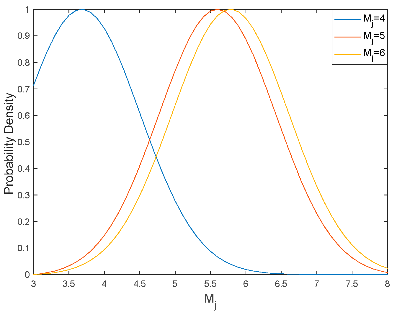
By substituting the results of Equation (15) into Equation (14), the magnitude probability density function of the average period parameter τc at time t can be obtained. Assuming that the earthquake magnitudes are Mj =4, Mj = 5, and Mj = 6, τc takes the values of 1.206, 2.1228 and 3.7359, respectively. Figure 2 presents the probability density distribution obtained by substituting the three magnitudes into Equation (13). The estimated magnitudes corresponding to the maximum probability density are 3.8, 5.6, and 5.8. The verification of the model reveals an error of 0.4836, resulting from the model and calculation errors. Thus, the earthquake magnitude can be predicted using Bayesian inference.

4.3. Predictive Simulation of PGV Based on Bayesian Inference

From the fitting results of Equation (8) and lgPd, the mathematical expectation μlgPd and standard deviation σlgPd can be expressed as:
μ l g P d = 0.9653 l g P G V + 0.0366 , σ l g P d = 0.1045 .
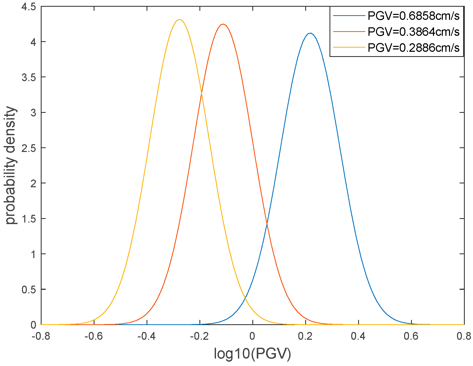
By substituting the parameters into Equation (14), the predicted PGV probability density function of the displacement amplitude parameter can be obtained. For PGV values of 0.6858, 0.3864, and 0.2886 cm/s, the lgPd values a
Are determined to be 0.2631, −0.0549 and −0.2139, respectively. The probability density distribution of different lgPGVs can be obtained by substituting these three displacement amplitudes into Equation (13) (Figure 3). The maximum probability densities of lgPGV are determined as −0.051, −0.3710, and −0.5310, with corresponding PGV values of 0.8892, 0.4256, and 0.2944 cm/s. Due to the large dispersion of the PGV data, the calculation and model errors are also relatively large.

4.4. Earthquake Judgment Model Based on Dual-Parameter Prediction

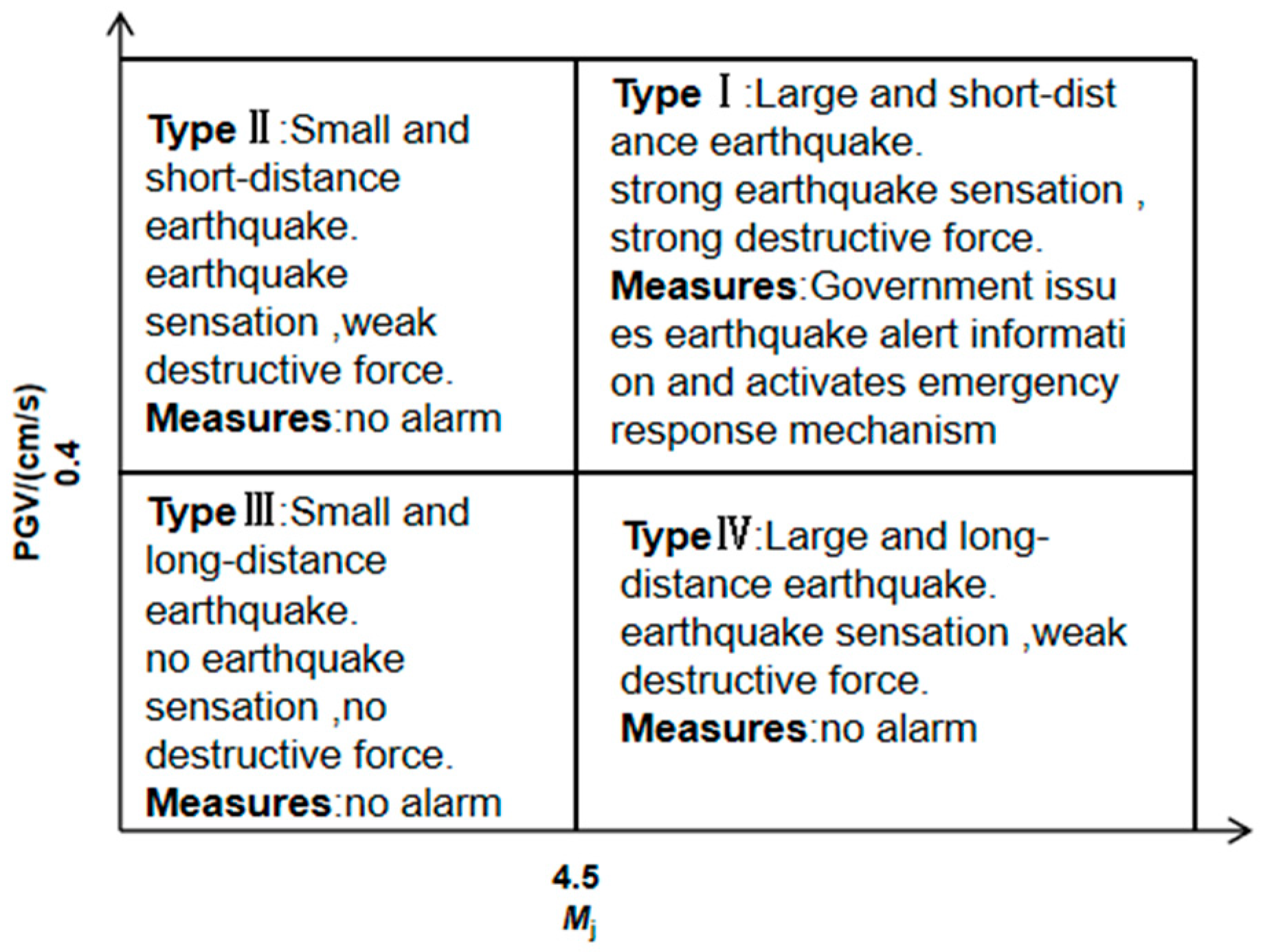
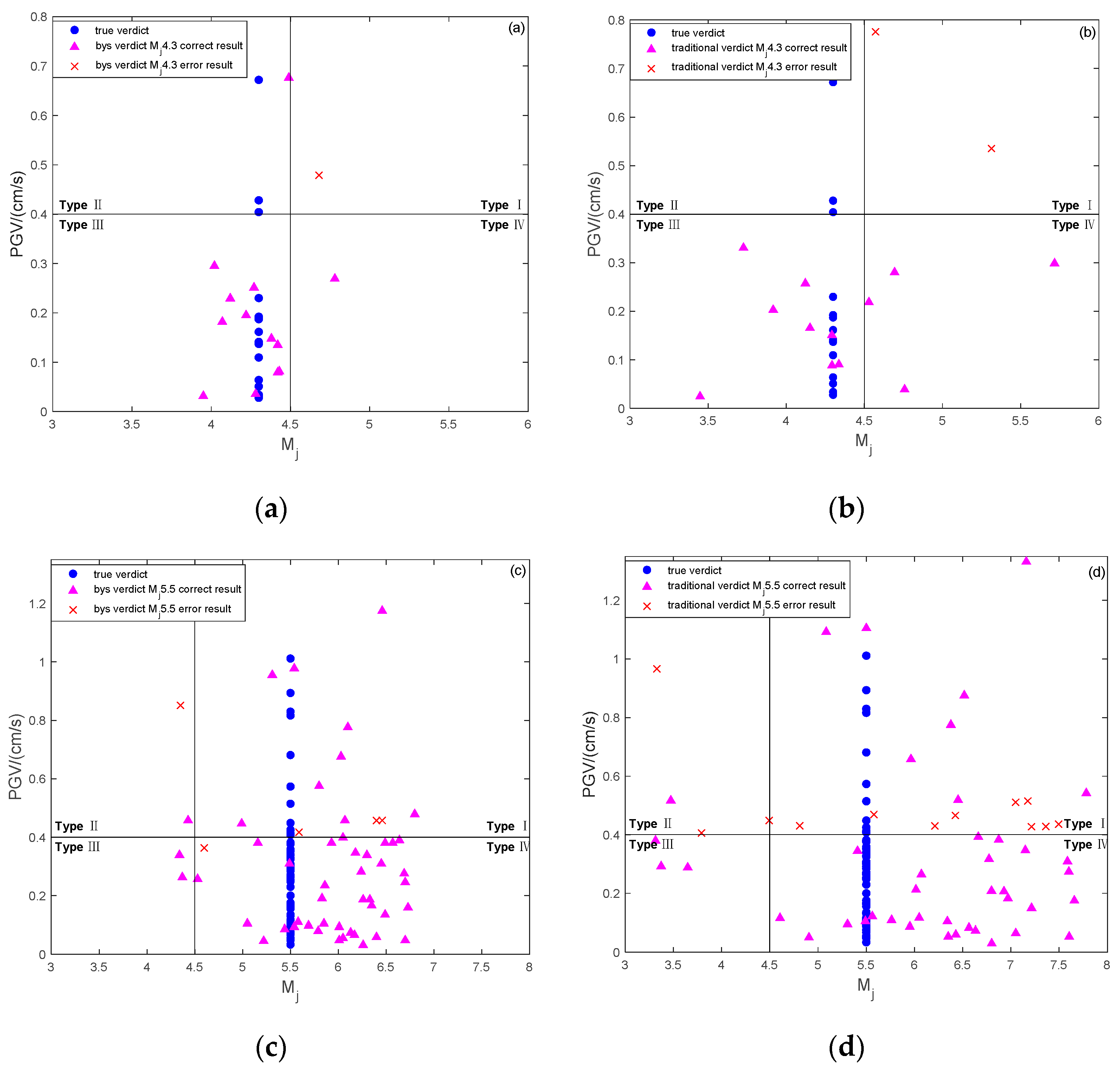
A judgment model was subsequently established to identify earthquake size and distance based on Zollo et al. [8]. According to the relationship between the early warning level and magnitude and intensity [17], the early warning values of magnitude and PGV were set. The seismic events can be classified into four types (Figure 4). In this paper, the thresholds were set as Mj = 4.5 and PGV = 0.4 cm/s. Figure 4 depicts the human sensation, damage degree, and corresponding earthquake warning measures of different earthquake types.

5. Comparative Testing and Analysis

Using the processed seismic data, the τc of the first-three-second P- wave is selected to obtain the predicted magnitude Mf using the traditional fitting approach. A dual-parameter prediction model based on Bayesian inference is then proposed to predict the earthquake magnitude Mb. Finally, the predicted magnitudes Mf and Mb are compared with the actual magnitude Mj. Figure 5 compares the corresponding dispersion degree and error distribution.
The standard deviation of the magnitude predicted using Bayesian inference is 0.3202 lower than that obtained by the traditional fitting method (Figure 5a). This reveals the results of the Bayesian prediction method to be more stable and reliable than those of the traditional fitting approach. The prediction method based on Bayesian inference exhibits a smaller distribution range of errors, a higher fitting accuracy, and a lower deviation degree, which can provide more accurate seismic parameter information for the four-level discriminant model (Figure 5b).
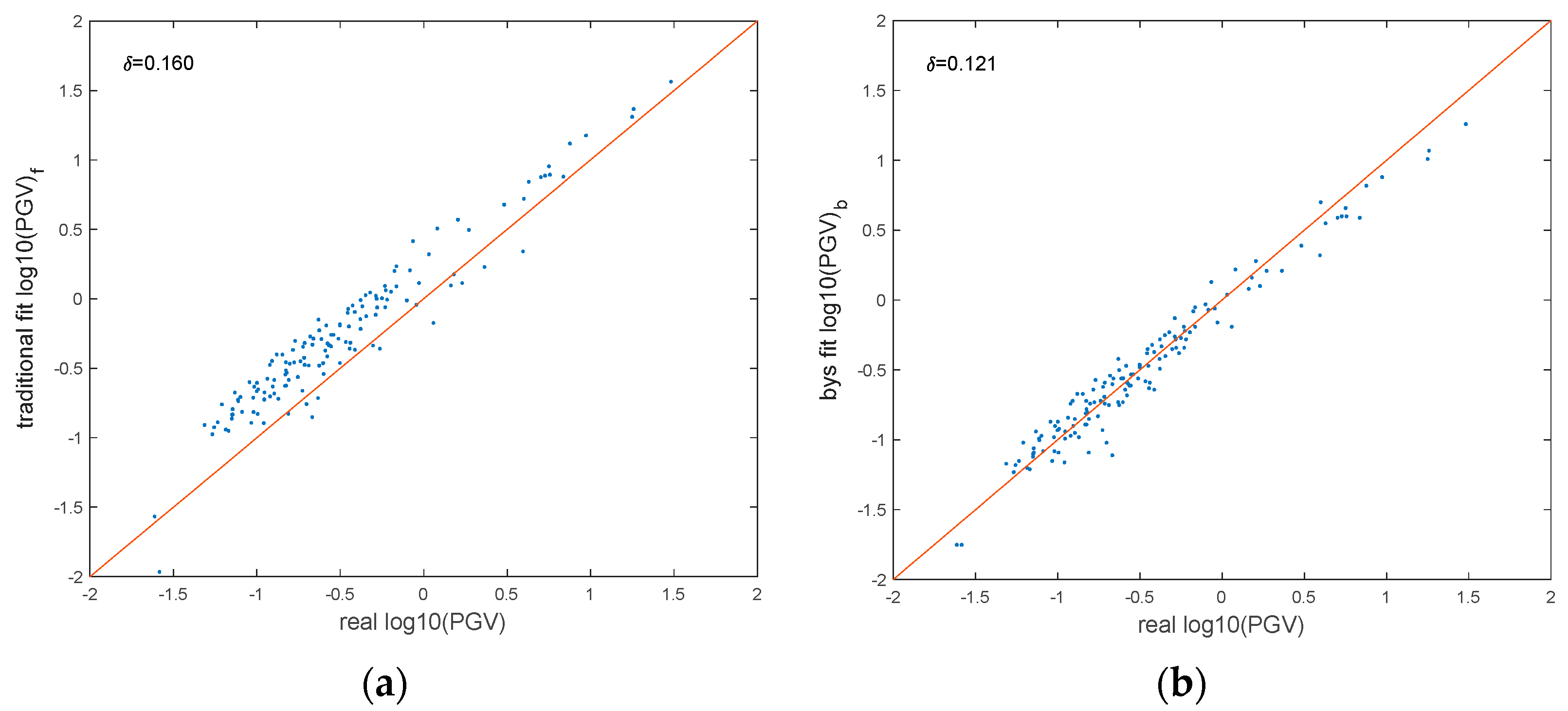
Similarly, by determining the Pd of the after-three-second P-wave, the PGV is predicted using the traditional fitting method (PGVf). PGV is then predicted according to Bayesian inference (PGVb). The predicted values obtained are then respectively compared with the real PGV. Figure 6 depicts the dispersion degree and error distribution. The slope of the red line in Figure 6a,b is 1, indicating that the Bayesian-inference-based PGV is more standard than that obtained with the traditional fitting method.

6. Discussion and Conclusions

In this paper, the 2014 Mj = 4.3 earthquake in Mt. Fuji, Japan (14 data points), and the 2017 Mj = 5.5 earthquake in Ibaraki, Japan (54 data points), were selected for the experimental analysis. Figure 7 displays the earthquake epicenters and the distribution of stations. The data of the first-three-second P- wave collected via 68 stations were selected to estimate the magnitude and PGV, and the earthquake hazard was predicted.
The values obtained with the Bayesian-inference-based prediction method and the traditional fitting method are substituted into the discriminative model in this paper. Figure 8 presents the distribution of all seismic hazard discrimination results. Table 1 shows the missed and false alarms of the Bayesian inference and traditional approaches.
Figure 8 and Table 1 reveal that both the Bayesian-inference-based prediction method and the traditional fitting method suffer from underreporting and misreporting. An under-prediction indicates that the estimated magnitude or PGV is smaller than the threshold and no earthquake alarm is issued, while actually the magnitude and PGV are greater than the threshold and an alarm should be issued. A false- prediction denotes that the estimated magnitude and PGV exceed the threshold and an earthquake alarm is issued, while actually the magnitude or PGV is smaller than the threshold and an alarm should not be issued. In the current 68 experimental results, the prediction method based on Bayesian inference has a miss rate of 2.94% and a false alarm rate of 5.88%; the conventional fitting method has a miss rate of 4.41% and a false alarm rate of 16.18%. The results are as follows: (1) The probabilistic algorithm founded on the predictive model of the magnitude from the average period (τc) and PGV from the displacement amplitude (Pd) from the initial 3 s of the P wave is able to provide a fast and accurate estimation of the final magnitude and location. (2) The Bayesian inference approach for the earthquake hazard discrimination model has a 2.94% miss rate and a 5.88% false alarm rate, which is lower than that of the traditional fitting method, thus increasing the accuracy and reliability of earthquake hazard estimation.
In this paper, a dual-parameter warning method of earthquake magnitude and PGV based on Bayesian inference is proposed to classify earthquake hazards into four levels. The results effectively improve the accuracy and reliability of early warning information. According to the real-time magnitude and PGV conditions, the τc and Pd of the first-three-second P-wave are fitted to the magnitude and PGV, respectively, and the empirical prediction formula is obtained. Furthermore, combined with historical earthquake information, the Gutenberg–Richter relationship is employed as the initial prior probability, and the τc and Pd of the first-three-second P- wave recorded in real time by the seismic station are used as the likelihood functions to predict the magnitude and PGV. The proposed method was compared with the traditional fitting approach [18], revealing the higher accuracy of the former. Finally, the Mj4.3 earthquake in the Mt. Fuji area and the Mj5.5 earthquake in the Ibaraki area of Japan were selected as examples to evaluate and discriminate the magnitude and distance of the earthquake and to analyze the under-prediction and false-prediction rates.
Despite the substantial progress made using the classification model of earthquake types in this paper, it has some limitations. For example, the early warning threshold needs to account for the characteristics of the local geographical environment, which vary across regions. This is particularly important, as the threshold settings play a large role in the model’s accuracy. Future research will focus on refining the model to further explore the available early warning indicators.

Author Contributions

Conceptualization and methodology, Z.L. and J.Y.; software, F.H. and Y.Z.; validation, F.H. and J.Y.; resources and data curation, Z.L., J.Y., F.H. and Y.Z.; writing—original draft preparation, Z.L. and J.Y.; writing—review and editing, Z.L., J.Y., F.H. and Y.Z.; supervision, Z.L. All authors have read and agreed to the published version of the manuscript.

Funding

Funding: This research was funded by National Natural Science Foundation of China, grant number 41874019.

Institutional Review Board Statement

Not applicable.

Informed Consent Statement

Not applicable.

Data Availability Statement

Earthquake data used in the study are available from Japan National Research Institute for Earth Science and Disaster Prevention: Available online: https://www.kyoshin.bosai.go.jp/kyoshin/quake/index_en.html (accessed on 6 July 2022).

Acknowledgments

We would like to thank the editor and reviewers for their valuable comments.

Conflicts of Interest

The authors declare no conflict of interest.

References

  1. Guo, K.; Wen, R.Z.; Peng, K.Y. Effectiveness evaluation and social benefits analyses on earthquake early warning system. Acta Seismol. Sin. 2016, 38, 146–154. [Google Scholar]
  2. Zhang, C.J.; Chen, H.Z.; Cai, J.A.; Hou, Y.Y.; Xu, H.H.; Li, W.D. Discussion on some issues of earthquake early warning engineering. J. Eng. Stud. 2014, 6, 344–370. [Google Scholar] [CrossRef]
  3. Zhang, H.C. Research on Key Technologies of Earthquake Early Warning System; Institute of Engineering Mechanics, China Earthquake Adminiistration: Harbin, China, 2013; pp. 1–190. [Google Scholar]
  4. Feng, J.W. Real-Time Estimation of the Ground Motion Field of Large Earthquakes; Institute of Engineering Mechanics, China Earthquake Adminiistration: Harbin, China, 2019; pp. 1–164. [Google Scholar]
  5. Kanamori, H. Real-time seismology and earthquake damage mitigation. Ann. Rev. Earth Planet Sci. 2005, 33, 195–214. [Google Scholar] [CrossRef] [Green Version]
  6. Zhao, C. Study on the Characteristics of P-Wave to Estimate Magnitude and PGA, PGV in the Field of Earthquake Early Warning; Southwest Jiaotong University: Chengdu, China, 2013; pp. 33–61. [Google Scholar]
  7. Iervolino, I.; Convertito, V.; Giorgio, M.; Manfredi, G.; Zollo, A. Real-time risk analysis for hybrid earthquake early warning systems. J. Earthq. Eng. 2006, 10, 867–875. [Google Scholar] [CrossRef] [Green Version]
  8. Wu, J.Q. Research on Progressive Ground Motion Intensity Warning Based on Bayes Principle and Characteristic Parameters of the P-Wave; Beijing Jiaotong University: Beijing, China, 2016; pp. 37–70. [Google Scholar]
  9. Zhou, Y.X.; Zhang, S.L.; Guo, K.; Zhang, Y. High speed train control strategy in earthquake early warning system. Technol. Earthq. Disaster Prev. 2015, 10, 116–125. [Google Scholar]
  10. Li, S.J.; Lü, Y.J.; Liu, J.W. Research on b-value statistical sample size in Gutenberg Richter law. Technol. Earthq. Disaster Prev. 2018, 13, 636–645. [Google Scholar]
  11. Zollo, A.; Amoroso, O.; Lancieri, M.; Wu, Y.M.; Kanamori, H. A threshold-based earthquake early warning using dense accelerometer networks. Geophys. J. Int. 2010, 183, 963–974. [Google Scholar] [CrossRef]
  12. Hao, M.X.; Zhou, Y.X.; Zhang, J.Z.; Zhang, K.; Yin, Z.J. Application of τc method in the early warning magnitude calculation in Inner Mongolia region. Earthouake Res. China 2020, 36, 136–145. [Google Scholar]
  13. Peng, C.Y.; Yang, J.S.; Zheng, Y.; Zhu, X.Y.; Xu, Z.Q.; Chen, Y. New τc regression relationship derived from all P wave time windows for rapid magnitude estimation. Geophys. Res. Lett. 2017, 44, 1724–1731. [Google Scholar]
  14. Long, C.H.; Lai, M.; Yu, H.; Li, D.H. Study on the correction between effective peak ground acceleration and seismic intensity. Earthq. Res. Sichuan 2011, 2, 26–31. [Google Scholar]
  15. Fang, J.Z.; Zhang, Y.; Wang, K.; Dong, Y. The Research on Application of Site Correction of Ground Motion in Rapid Reporting of Seismic Intensity. South China J. Seismol. 2020, 40, 17–26. [Google Scholar]
  16. Ma, Q.; Li, S.L.; Li, S.Y.; Tao, D.W. On the correlation of ground motion parameters with seismic intensity. Earthq. Eng. Eng. Dyn. 2014, 34, 83–92. [Google Scholar]
  17. Song, J.D.; Jiao, C.C.; Li, S.Y.; Hou, B.R. Prediction method of first-level earthquake warning for high speed railway based on two-parameter threshold of seismic P-wave. China Railw. Sci. 2018, 39, 138–144. [Google Scholar]
  18. Wang, Y.W.; Li, X.J.; Cao, Z.Z.; Lan, J.Y.; Liu, J. Continuous estimation magnitude for earthquake early warning based on Kik-net borehole bedrock strong motions. Earthq. Eng. Eng. Dyn. 2020, 40, 42–52. [Google Scholar]
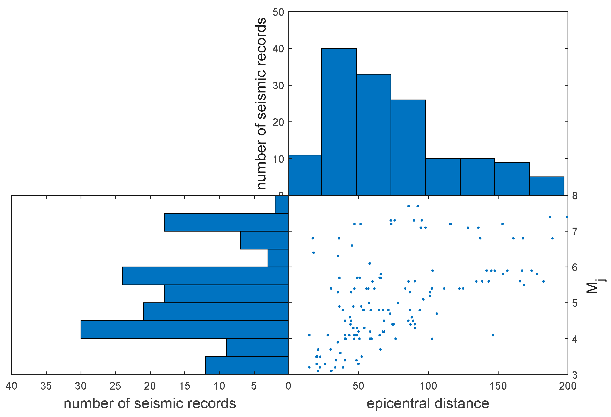
Figure 1. Distribution of the number of earthquake records with selected epicentral distances and magnitudes.
Applsci 12 12849 g001
Figure 2. Probability density distribution of different Mj earthquake early warning method based on Bayesian inference.
Applsci 12 12849 g002
Figure 3. Probability density distribution of different lgPGVs.
Applsci 12 12849 g003
Figure 4. Seismic judgment model.
Applsci 12 12849 g004
Figure 5. Comparison of the actual magnitude and the predicted magnitude using the conventional method and the Bayesian inference method (a) and its error distribution (b).
Applsci 12 12849 g005
Figure 6. Comparison of true PGV with conventional fitted predictions (a) and Bayesian-inference-based predictions (b).
Applsci 12 12849 g006
Figure 7. Distribution of epicenter stations for magnitudes Mj4.3 (a) and Mj5.5 (b). Available online: www.kyoshin.bosai.go.jp (accessed on 6 July 2022).
Applsci 12 12849 g007
Figure 8. Comparison of the results obtained from the Bayesian-inference-based prediction methods (a,c) and the traditional fitting methods (b,d) with the true discriminant results.
Applsci 12 12849 g008
Table 1. Comparison of missed and false alarms of the experimental results of the two methods.
Missed AlarmFalse Alarm
Number of Missed AlarmsMissed Alarm RateNumber of False AlarmsFalse Alarm Rate
Bayesian prediction method22.94%45.88%
Traditional fitting method34.41%1116.18%
Publisher’s Note: MDPI stays neutral with regard to jurisdictional claims in published maps and institutional affiliations.