Methodology for a Numerical Multidimensional Optimization of a Mixer Coupled to a Compressor for Its Integrationin a Hyperloop Vehicle

Featured Application

hyperloop powertrain.

Abstract

The current environmental concern has led both the industry and researchers to look for alternate means of transport. Amongst them, the hyperloop has become a quite promising idea. In order to overcome some of its limitations, including a compressor in its propulsive system has been investigated. In this paper, a strategy to improve the design of the mixer, which will blend the bypass and core streams coming out of the compressor, was addressed. Due to the lack of ad hoc compressors and the impossibility of experimental testing, a multidimensional optimization methodology with CFD tools was developed. A Taguchi DOE was employed for a preliminary 2D optimization from an initial geometry, whereas a numerical adjoint method was explored for the whole 3D mixer. By using this method, an initial decrease in the pressure drop of $16\%$ was obtained with the 2D stage, whereas an additional $10\%$ reduction was achieved in the 3D optimization. With this, the propulsive efficiency of the whole hyperloop system will be improved.

1. Introduction

In the last century, the transport environment has been dominated by fossil fuels and their respective combustion propulsion systems. At the very beginning, this concept became a revolution because of its distinctive speed and comfort in comparison to previous means of transport. Nevertheless, with globalization and the easy access to these technologies, nowadays there is a situation where the excess of traditional fuel-propelled vehicles, not only cars, but also planes or trains, is having a huge impact on the environmental situation [1], and the predictions indicate that this will increase due to the higher energy demand [2], setting an alarm about its prejudicial influence on nature and the worrying high levels of CO${}_2$ emissions [3]. Because of these reasons, in the last years, the community has turned its efforts into the development of new environmentally friendly means of transports [4] and alternative ways of propulsion [2,4]. Amongst them, the concept of hyperloop appeared in 2013 [5]. This idea of vactrain (or vacuum tube trains), although it has its origins in the past [6], consists of the concept of a high-speed train travelling through a tube in partial vacuum in order to minimize the drag problems derived from the high velocities. In the next years, the feasibility of the idea was studied by several investigators [7], and a few aerodynamic and thermal analyses have been performed [8]. Many different ideas have been developed about the propulsive systems, such as electric power fed by solar panels [9] to electromagnetism for a suspension system [10,11] that avoids the friction losses which could become a limiting variable at high speeds.

Therefore, the environmental benefits derived from a technology with these characteristics are straightforward. Moreover, the possibility of reaching high speeds by ground travelling, with the comfort advantages it implies, also constitutes a fundamental advantage against its apparent main market rival, air transport [12]. Even in the case of developing nicer air transport satisfying environmental requirements, the overall time spent is way longer than travelling by ground, not only because of transportation itself (take off, ascent, descent…), but also for the particularities of the part where the individual leaves their initial location until the boarding is completed.

Nevertheless, the fact that it is a relatively new concept implies the apparition of new problems, some of them typical from other technologies that are translated to the hyperloop concept.

The main challenge that the hyperloop is facing is the concept of the Kantrowitz limit [13]. Whereas technologies such as open-air high-speed trains or air transport itself has no chocking problems due to external flow, a pod travelling through a closed tube at high speed could cause a choking of the flow when supersonic conditions are reached. Once the flow arrives at the constriction of a section between the tube and the pod, as the frontal area is reduced, the velocity must increase. In consequence, it could lead to a choke of the flow at certain points of the area contraction, making the pod act like a closed piston [14,15]. This would lead to a huge increase in the drag of the vehicle, nullifying all the aerodynamic initial advantages of the hyperloop concept. Therefore, the Kantrowitz limit acts as a maximum speed limit the hyperloop can develop in order to avoid these prejudicial effects. By developing conservation equations, the Kantrowitz limit would be defined with the relation of the flow speed and the quotient between the frontal area of the tube and the pod, commonly known as blockage ratio.

Therefore, the Kantrowitz limit being the main limiting phenomenon of the hyperloop development, it has become the main investigated topic, with proposed solutions such as the utilization of aeronautical elements by adding airfoils to the external structure [16] or the optimization of the external pod [17,18] and the effect of this shape on the wave phenomenon [19].

However, in the context of the present paper, amongst these proposed solutions, the most interesting one is the proposal of using a compressor [20,21]. It shows that by implementing an air bypass system such as a compressor that crosses the pod, the air passing through the area between the pod and the tube will be reduced, and therefore the velocity of the pod could be increased [22,23]. Moreover, the larger the flow that the compressor is able to handle, the greater the drag reduction. However, within the found literature, the problem of the adaptation of a compressor in the internal aerodynamic system has not been addressed, as these works [20,21,22,23] consider the compressor and the nozzle by means of a simple model in which some mass flow is swallowed at the vehicle front and discharged at its rear part. The current work therefore predicts for the first time the flow field in the compressor and the downstream geometry in the framework of a hyperloop system.

Then, once the solution of using a compressor is exposed, the next step would be its implementation. Nevertheless, this brand-new idea leads to new problems: both the lack of compressors for cases with these characteristics, as they are deeply developed in Appendix A, and the lack of completely designed pods adapted to have a compressor that would allow a test of this concept in wind tunnels.

On the other hand, the main advances in CFD calculations make the characterization of the compressor map and performance possible [24], potentially overcoming the second problem. With respect to the lack of ad hoc compressors, this present paper proposes the adaptation of existing compressors to the original hyperloop flow properties. Because of the characteristics of the incoming flow, an axial compressor typical of air engines is the best option. As a result, this paper addresses the new problem of the design of a mixer downstream of the compressor, which allows the implementation of an axial compressor by maintaining, within the possibilities, the achieved compression and mix the two currents in order to, later, being expelled by the nozzle. To the author’s knowledge, such a core-to-bypass flow mixer represents a new concept for the hyperloop, and due to its novelty, it has not been investigated. In order to overcome these problems, several hypotheses are taken, and a suitable optimization strategy is proposed in several stages.

In conclusion, the outlined challenges shown in Section 1, together with the appendix, serve as a motivation for the investigations in the next sections. In Section 2, a general view of the paper is provided, including the system description and the optimization strategy. In Section 3, the numerical model is developed, discussing the CFD methodology, the physical models that govern the case and the assumptions made for the feasibility of the optimization process. In Section 4, the chosen optimization process for both the 2D and 3D cases is theoretically developed by exposing not only the method itself, but the reasons of its choice. In Section 5, the results of the optimization process are shown. Once again, the 2D and the 3D are justified separately and, finally, a simulation of the whole compressor and mixer system is used to complete the process. Finally, Section 6 tries to synthesize the main conclusions of the present paper, as well as present future work.

2. Overview of System Description and Optimization Approach

In this section, an overview of the problem faced by this paper is provided.

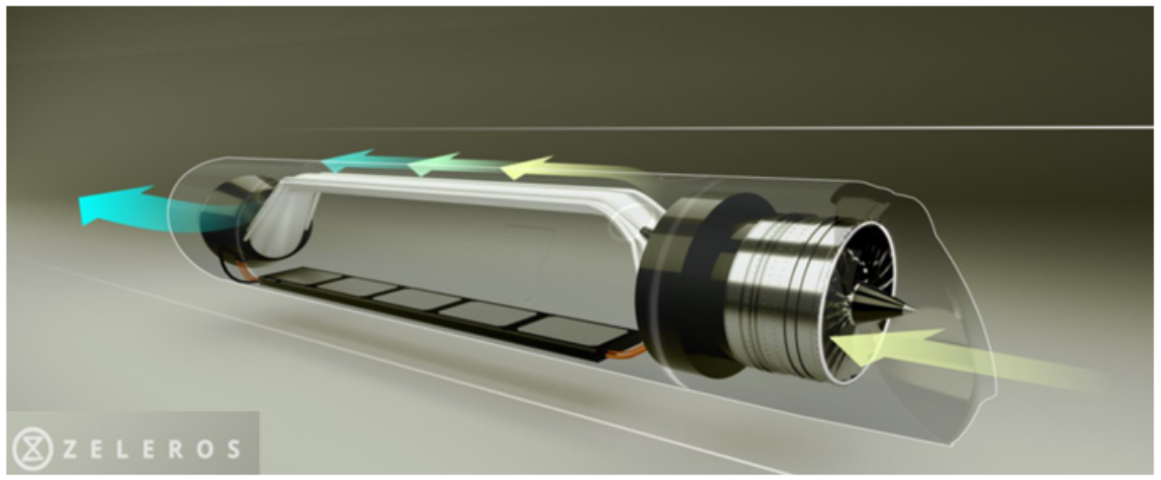
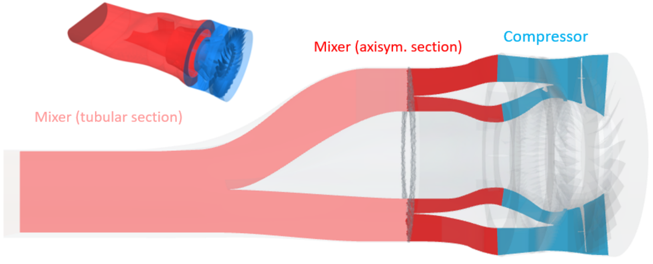
As it was introduced in Section 1, the issue of the Kantrowitz limit could be improved by adding a compressor to the propulsive system. As it is shown in Figure 1, the outlet of the compressor needs a geometry that readapts the two streams coming out of the compressor in order to conduct the air towards the nozzle at the outlet part of the pod. Therefore, the design of this body—from now on known as the mixer—is the main objective of this paper. For that, Figure 2 reflects the geometry domain that is modelled, making the differentiation between the compressor and the mixer.

Having the overall problem in mind, a multidimensional geometrical optimization is proposed after exploring the following two approximations:

• Coupled: Both the compressor and the mixer are simulated simultaneously. The main advantage lays in the fact that the possible effects that the mixer may have upstream on the compressor are completely taken into account. Nevertheless, the computational cost of a problem of these characteristics makes an approach like this impossible, as the number of required cells would increase by more than an order of magnitude. With the independent mesh as established in Section 3.4, the compressor cell has around 80M elements, whereas the mixer is properly solved with only 1M elements.
• Uncoupled: The main hypothesis consists in assuming that the mixer has no relevant upstream impact on the compressor. As a consequence, the mixer can be calculated by just imposing the outlet conditions of a previous simulation of the compressor alone, diminishing considerably the computational cost.

Considering the extensive optimization numerical campaign of more than 100 simulations conducted in Section 4, the coupled option was not affordable due to the significant increase in computational effort. In consequence, the authors opted for the second option. Indeed, each simulation, adding the time employed in both the mesh of each possible geometry and the calculation of the solution, would cost 40× the computational effort of the mixer alone.

With respect to the chosen approach, the next algorithm flowchart summarized in Figure 3 was developed throughout the following methodology:

• Base geometry.
• Obtaining the BC values: after a preliminary design is proposed, the boundary conditions from its design together with the compressor are obtained in order to start the process.
• Optimization:

  −

  First optimization (2D): A Taguchi DoE (design of experiments) is implemented for a first optimization of the axisymmetric parts of the mixer.

  −

  Second optimization (3D): by using an adjoint method, an optimization of the 3D complete mixer is carried out.

• Coupling evaluation.

3. Numerical Configuration

3.1. Meshing Strategy

3.1.1. Mesh Configuration 3D

Figure 2 shows the division between the existing compressor, in blue, and both parts of the mixer, in red, whose geometric optimization is the main objective of the present paper.

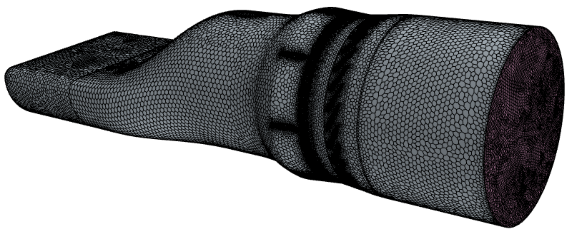
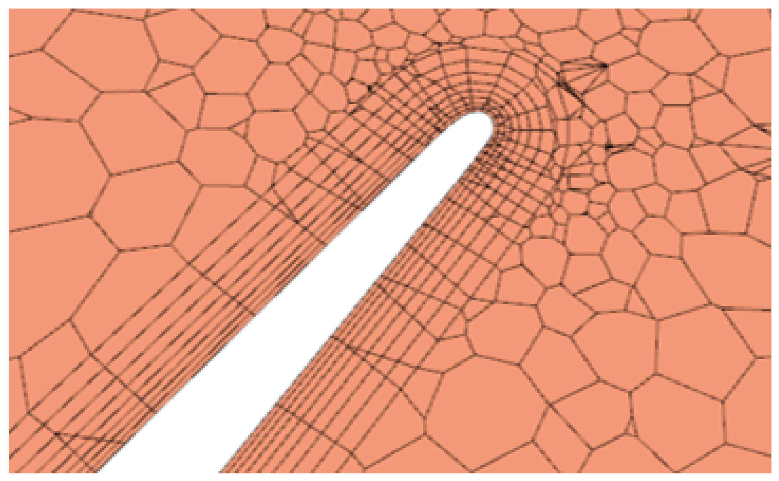
For the sake of consistency, the geometry was divided in several sections. Thus, in order to determine the different reference systems for the movement, the same mesh size was imposed at the interfaces between the different sections. However, as it can be seen in Figure 4, the sections which englobed the rotor and the stator were refined with respect the rest of the geometry. As a result, a base mesh composed of polyhedral cells was used, with a base size of 0.1 mm in general and 0.001 mm in the most critical sections, close to the blades of the compressor. Moreover, in order to increase the resolution in the blades, the curvature of the surface mesh in the blades was highly refined, increasing considerably the number of elements in these zones, as shown in Figure 5. Prism layers were configured on the walls, achieving a mean y+ value in the chosen mesh of 1.7, close to the ideal of 1.

3.1.2. Mesh Configuration 2D

As is justified in Section 4, there was a stage where a 2D axisymmetric geometry was used for its optimization. Figure 6 shows the used domain, where the dashed line marks the correspondent axisymmetric part of the original geometry. Therefore, a 2D mesh configuration with its correspondent independence process was also needed. The chosen mesh followed a configuration analogous to the 3D case, using polygonal elements and a prism layer mesh looking for y+ = 1 and a maximum aspect ratio around 50.

3.2. Physical and Numerical Configuration

Before starting with the setup of the case, the nature of the novelty of the application must be considered, meaning that some hypotheses widely accepted for modelling conventional means of transportation could be invalid in the framework of the current paper. As it was previously stated, the pressure conditions inside the tube of the hyperloop are considerably lower than the atmospheric pressure. At this point, the main hyperloop projects have considered an operating pressure of about 0.1 atm [15,20]. Therefore, the continuum hypothesis for such air could be questioned. For that, it is common to check the Knudsen number. Previous works in the field of hyperloop research have already confirmed that according to that number, this low-pressure air can be accurately modelled as a fluid continuum [20,25].

For the spatial discretization, the finite-volume approach of CFD software SIMCENTER STAR-CCM+ was employed, selecting a second-order implicit scheme solved as a density-based flow due to the remarkable compressible behaviour. With respect to the temporal discretization, the nature of the case allowed the simplification of assuming steady conditions, as the objective point was the compressor design condition, where the flow tends to behave quite stably and steady. As for the turbulence treatment, one could solve some turbulent scales using a detached eddy simulation (DES) [26] or even a large eddy simulation (LES). Nevertheless, a RANS model of the turbulence using a k-w SST configuration [27] should be enough to achieve a reasonable trade-off between accuracy and computational time [28,29]. Indeed, the usage of such turbulence model has been validated in the framework of axial compressors [28] and internal flow mixing problems [30], which, if combined, would reduce the impact of the lack of experimental validation in the scope of the current problem, since no compressor-assisted hyperloop prototype systems exist. Moreover, with the aim of improving the similarity with real conditions, a laminar-turbulent transition model was added with the objective to capture the behaviour in those zones where, especially in the later 3D model with the compressor, the flow presents a laminar condition. Is it worth mentioning that, traditionally, a turbulent transition model asks for a finer mesh, but taking a look at the geometry of the compressor, this was not the main limitation.

3.3. Boundary Conditions

The imposed boundary conditions must be divided between the main optimization cases, where the mixer is calculated alone and the final case with the compressor and the mixer.

3.3.1. Compressor

In order to get the flow conditions at the outlet of the compressor that would serve as inlet boundary conditions to the mixer, a simulation of the design point in the compressor alone was needed.

In this case, the total pressure at the inlet (12 kPa) was imposed, coming from the upstream flow conditions of the operational performance of the hyperloop, that is, the sum of the environment static pressure of 10 kPa plus the additional compression upstream of the compressor induced by the pod, which, together with the dynamic term due to the pod reference velocity of 125 m/s, provided those additional 2 kPa, whereas the pressure at the outlet was modified until the objective mass flow given by the design point of the compressor (5.92 kg/s) was achieved.

With respect to the movement of the rotor, several strategies are found in the literature and they can be divided in a transient configuration, known as rigid body motion (RBM) [31,32], and a steady configuration with a moving reference frame (MRF). This one, in turn, is divided in two possible options: a frozen rotor [33] or a mixing plane (MP) [34]. In this work, knowing the stability of the selected point, which was, presumably, a design point, some simplifications could be taken in order to maintain a reasonable computational time. Thus, amongst all the options, it was opted for using an MRF with a mixing plane to simulate the rotation of the rotor, as it should be accurate enough at design points [35]. By doing so, the configuration of the case remained in steady conditions, and the movement of the rotor was simulated by referring the rotor itself to this new MRF–mixing plane (N = 11,000 rpm).

3.3.2. Mixer BC

The simulations with the mixer alone, on the other hand, required a different setup of the conditions.

The given data coming from the compressor provided the averaged circumferential velocity components and temperature distributions in both the bypass and the core inlet. In the next section, how these distributions were obtained is explained. In consequence, in order to respect the compressor outlet conditions in the mixer with the objective to get over the coupling of the two components, these distributions were imposed at the inlet of the mixer. Paying attention to the other hypothesis, which fixed the mass flow and the BPR, this mass flow should be imposed in the outlet. Nevertheless, due to numerical stability reasons, a pressure outlet condition was selected with a mass flow controller, in order to find the static pressure corresponding to the desired mass flow.

3.3.3. Compressor and Mixer BC

The whole group of compressor and mixer together followed a conjunction of the two other configuration for its boundary conditions, that is, a total pressure inlet of 12 kPa, the same motion configuration for the rotor and a pressure outlet modified in order to get the objective mass flow of 5.92 kg/s.

3.4. Independence of Mesh

Once the meshing strategy and configuration were exposed, as well as the determination of the boundary conditions, the next step consisted in ensuring the independence of the spatial discretization. Three possible mesh sizes were calculated in order to check the independence mesh. In

Table 1. Independence of the 3D mesh.

Variable	Coarse (25M Cells)	Medium (75M Cells)	Fine (155M Cells)
$\dot{\mathit{m}}$(kg/s)	5.886	5.92	5.92
$\mathit{BPR}(-)$	2.61	2.55	2.55
${\mathit{P}}_{\mathit{t},\mathit{outlet}}$(Pa)	15,550	16,490	16,500
${\mathit{P}}_{\mathit{t},\mathit{core}}$(Pa)	16,601	17,200	17,160
${\mathit{P}}_{\mathit{t},\mathit{bypass}}$(Pa)	16,031	16,649	16,612
${\mathbf{\pi }}_{\mathit{t}-\mathit{t}}(-)$	1.29	1.37	1.37
${\mathbf{\pi }}_{\mathit{core}}(-)$	1.38	1.43	1.43
${\mathbf{\pi }}_{\mathit{bypass}}(-)$	1.33	1.385	1.385
${\mathbf{\eta }}_{\mathit{t}-\mathit{t}}(-)$	0.7	0.73	0.73
${\mathbf{\eta }}_{\mathit{core}}(-)$	0.75	0.8	0.8
${\mathbf{\eta }}_{\mathit{bypass}}(-)$	0.68	0.72	0.72

, the main averaged values are included. It is worth mentioning that the inlet referred to the inlet of the whole compressor (total), the outlet of the core (core) and the outlet of the bypass (bypass), whereas the outlet always referred to the outlet of the mixer.

$${\pi }_t=\frac{P_{t,outlet}}{P_{t,inlet}}$$

(1)

$${\eta }_t=\frac{{\pi }_{t-t}^{\frac{\gamma -1}{\gamma }}}{\frac{T_{t,outlet}}{T_{t,inlet}}-1}$$

(2)

$$BPR=\frac{{\dot{m}}_{bypass}}{{\dot{m}}_{core}}$$

(3)

From the differences obtained between the 3 different meshes, with a general difference of about $3\%$ between the first two meshes and almost no variance with the fine mesh, it can be concluded that the medium mesh already achieved mesh independence and was therefore used.

An analogous process was performed for the 2D axisymmetric mesh, and the obtained results are summed up in the next table. By looking at

Table 2. Independence of the 2D mesh.

Variable	Coarse (9k Cells)	Medium (19k Cells)	Fine (40k Cells)
$\dot{\mathit{m}}$(kg/s)	3.73	3.746	3.741
$\mathit{BPR}(-)$	2.61	2.55	2.55
${\mathit{P}}_{\mathit{t},\mathit{outlet}}$(Pa)	5730	5771	5778
${\mathit{P}}_{\mathit{t},\mathit{core}}$(Pa)	8380	8311	8240
${\mathit{P}}_{\mathit{t},\mathit{bypass}}$(Pa)	4738	4790	4810

, the chosen mesh was the medium mesh. It could be reasoned that, as the differences between the coarse and the medium mesh were all around $1\%$, except for the BPR, where the difference was up to $3\%$, the coarse one already reached independence. Nevertheless, as the number of elements was still low in the next one, and looking for future possible calculations, the second one was chosen, which presented almost negligible differences in comparison with the last mesh tested.

4. Optimization Process

4.1. Strategy

In Section 2, the problem was described in detail together with the way to face it. Therefore, following those ideas and the algorithm flowchart from Figure 3, the strategy is exposed in full detail in this section.

4.2. 2D Initial Geometry

A 0D-based design of the mixer was done as a first step. After obtaining the average properties of the flow at the mixer input, different approaches for the design were evaluated. For every approach, the flow evolution was considered isentropic, the mass was conserved along the flow channels and no bleeding occurred. Secondly, several design strategies were proposed for the initial mixer in order to obtain an initial geometry that, even for the beginning, provided a promising solution:

D1:

Isobaric mixer: the objective was to design a mixing area such that it matches the static pressure of the core and bypass streams of the flow.

D2:

Isospeed mixer: in this design, the mixing areas were imposed so the velocities of the flow streams coincided.

D3:

Iso-$\mathbf{\rho }·\mathit{v}$ mixer: in this design, the mixing areas were imposed so the product of velocity and local density of the flow streams coincided.

D4:

Isomomentum mixer: this design guaranteed that the axial momentum of the bypass and core flow streams was the same by varying the mixing section areas.

D5:

Custom mixer: For this design a custom weighted optimization process was performed to vary the mixing areas. The weights were applied to the stream velocity difference, stream static pressure difference and target outlet velocity. The relative respective weights applied were 1, 5, and 3.

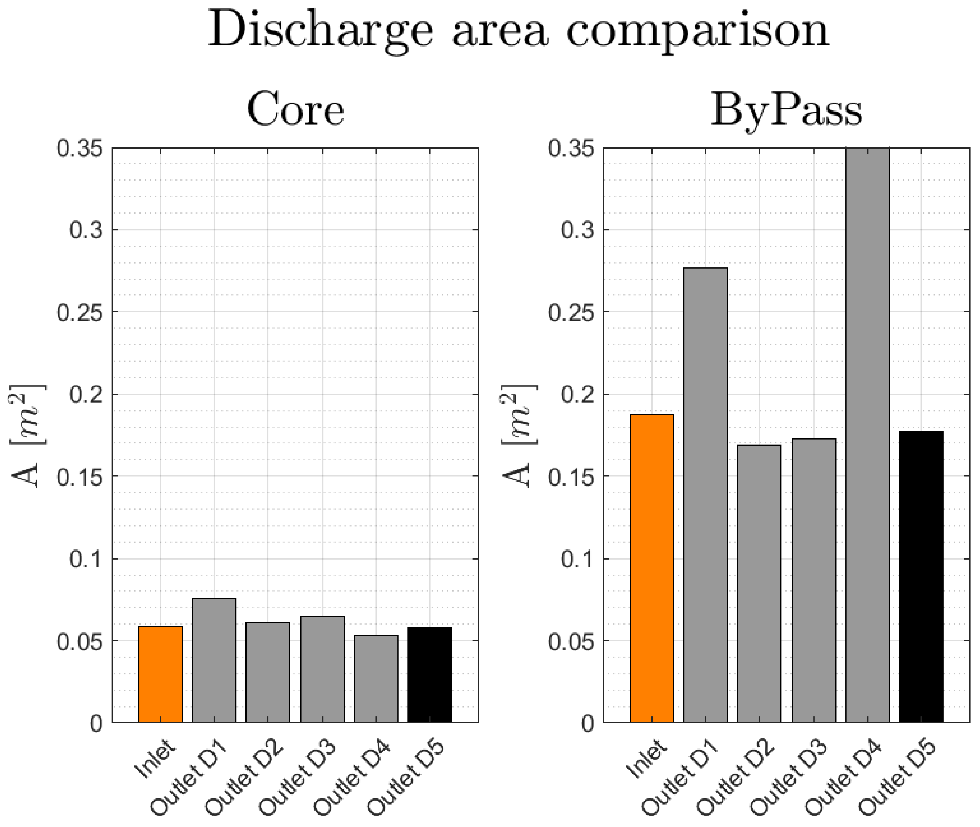
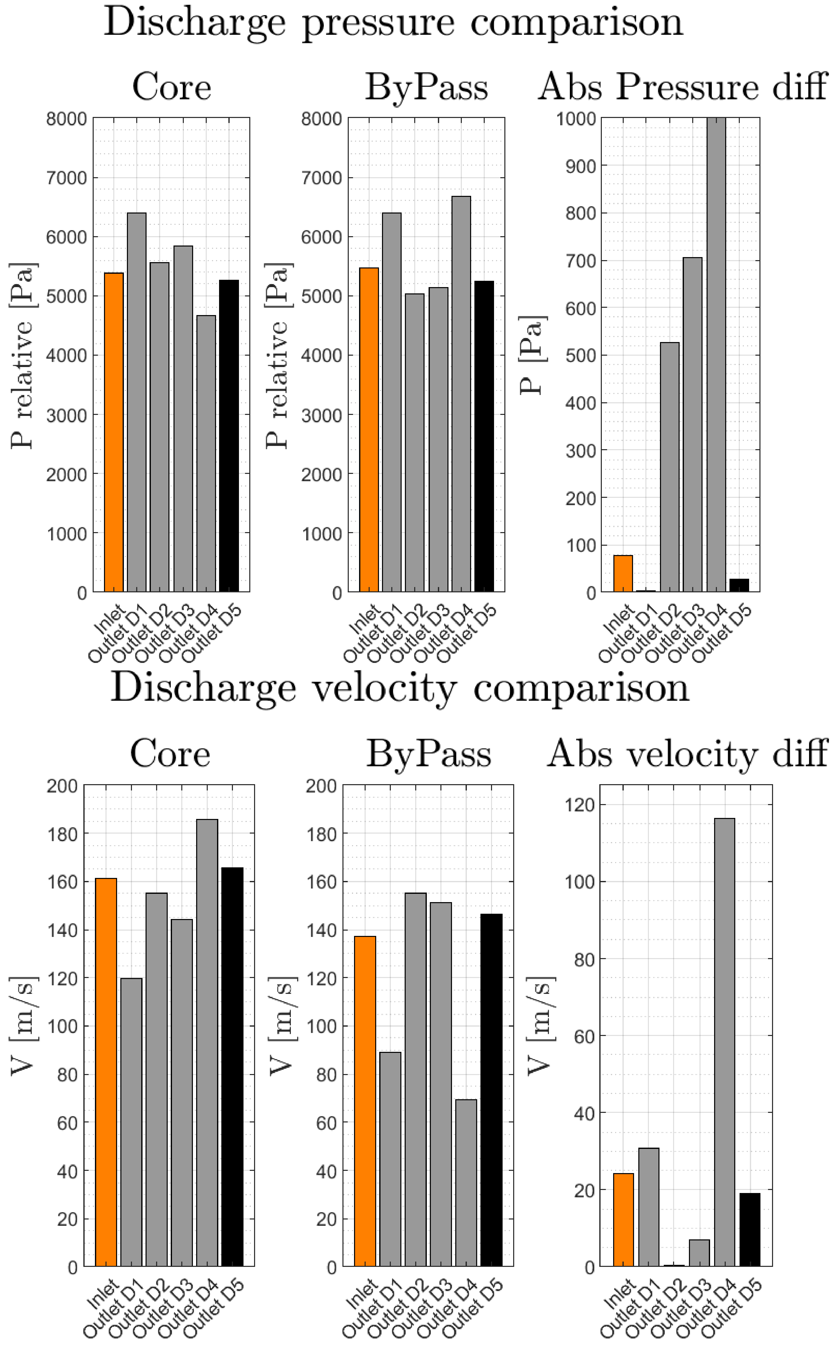
After evaluating each design (see Figure 7), it was decided to use the custom approach because, as it can be observed, it achieved a good compromise between the discharge pressure comparison—almost equal to the isobaric configuration—and the velocity difference between both branches.

4.3. 2D Optimization Stage

In the present paper, a multidimensional optimization strategy is proposed in order to reduce the computational time needed. From the initial geometry in Figure 2, it was observed that there was a subdivision in the geometry itself. A first part presented an annular distribution where the primary and the secondary flows were mixed, whereas there was a second transitional tubular section where the flow abandoned its annular character.

The results obtained at the inlet of the mixer were used as inputs in the isolated mixer to be optimized.

From previous existing simulations of an isolated version of the compressor, the circumferential and radial distributions of pressure, temperature and velocity components were obtained. For both core flow and bypass channel flow, the velocity averaging was performed as:

$$v_x\left(r_i\right)=\frac{1}{2\pi }{\int }_{-\pi }^{\pi }\left|\overrightarrow{V_x(r_i,\theta )}\right|d\theta$$

(4)

$$v_r\left(r_i\right)=\frac{1}{2\pi }{\int }_{-\pi }^{\pi }\overrightarrow{(V_y(r_i,\theta ),V_z(r_i,\theta ))}·\overrightarrow{\left(\right(cos\left(\theta \right),sin\left(\theta \right))}d\theta$$

(5)

$$v_{\theta }\left(r_i\right)=\frac{1}{2\pi }{\int }_{-\pi }^{\pi }\overrightarrow{(V_y(r_i,\theta ),V_z(r_i,\theta ))}·\overrightarrow{\left(\right(-sin\left(\theta \right),cos\left(\theta \right))}d\theta$$

(6)

Moreover, the pressure and temperature averaging were, respectively, computed as:

$$p\left(r_i\right)=\frac{1}{2\pi }{\int }_{-\pi }^{\pi }P(r_i,\theta )d\theta$$

(7)

$$T\left(r_i\right)=\frac{1}{2\pi }{\int }_{-\pi }^{\pi }T(r_i,\theta )d\theta$$

(8)

Once the pressure, temperature and velocity average distributions were obtained, they needed to be transformed as the original compressor simulation was performed on a revision of the geometry without the real component discharge areas. Because of this, the boundary conditions for the mixer design were adapted as follows:

• The updated average Mach number in the core and bypass stations was calculated using the conservation of mass equation assuming isentropic flow.
• Assuming a conservation of the total temperature, the updated static temperature was calculated from the CFD case total temperature and the updated Mach number from the first step.
• The updated static pressures were calculated using the isentropic relations and the CFD case total pressure.
• The updated density was computed with the equation of state for an ideal gas.
• The flow axial velocity was calculated using the continuity equation and the updated density.

The boundary conditions for the CFD cases were obtained as follows. Firstly, all of them were conformally mapped onto the correct radii range from the original compressor CFD radii for the bypass and core streams. Then, each of them was accordingly scaled: the axial velocity, scaled to preserve the average obtained axial inlet speed; the radial and tangential velocity, scaled to preserve the angular momentum of the flow streams; and the static pressure and temperature, scaled by the ratio of the updated area and average value from the original CFD case of static pressure and temperature, respectively.

The obtained profiles were used in the following stages of optimization and CFD calculations.

Every optimization process is divided in several substages. In the present paper, we opted for a conventional first approximation and the initial step consisted in determining which variables to study. The initial 2D proposed geometry was built from quadratic segment splines with 3 points each. In consequence, following the mixer shape, it led to a geometry of 11 points. Each point, as it was part of the spline, presented 4 variables: X and Y position, angle and curvature. This meant, when using a full factorial design of experiments, a control points set of 55 which, by using a high, a medium and a lower level, would imply a completely unaffordable set of cases. In consequence, by observing the geometry and taking some hypotheses, such as geometric restrictions, the continuity in the curvature of the splines and tangencies, the control variables were reduced to 13, as shown in Figure 8.

From there, several design of experiments (DoE) strategies were employed in the framework of CFD optimizations: full factorial design [36], fractional factorial design [37], Taguchi’s method [38,39] and even more complex methods [40].

By looking at the characteristics of each of the cases assessed, the Taguchi method was selected due to its convenience for the case considered in the present paper.

4.3.1. Taguchi Method

The Taguchi method [41] was originally intended for quality issues, and it has already been used for engineering before [42]. Unlike other simpler methods such as the factorial designs, the Taguchi method tests pair of combinations from all the possible combinations by a method where the parameters and levels are organized in orthogonal arrays that do not consider the interaction between the variables. By implementing the method, it can be computed how much each of the parameters affects the mean and the variance of the process and use it as a quality factor of the method itself.

The steps of a regular Taguchi method are developed as follows:

• Determine the maximum or minimum target function. In this present paper, the goal was the minimization of the total pressure drop between the inlet of the mixer and the outlet.
• Determine the variables involved, developed previously in this same section, along with the levels of each variable, as well as the levels imposed for each variable. These parameters are shown in Figure 8; they were geometrical parameters that determined the geometry, whereas the levels were selected by trial and error in order to avoid nonsense bodies.
• Select the orthogonal array. The Taguchi methods usually provides an established set of orthogonal arrays that the user can use according to the number of variables and levels. In this case, the use of 13 variables with 4 levels each led to an orthogonal array of L64.
• Evaluate the mathematical method and the computation of the variables to provide information about the quality of the process. In this case, once the method was performed, the influence of each of the variables was evaluated by calculating the corresponding sound/noise function for minimizing studies, which could be used for a second optimization round if needed:

  $$S{N}_i=-10·log\sum _{u=1}^{N_i}\frac{y_u^2}{N_i}$$

  (9)

  where i is the experimental number, u is the trial number and N is the number of trials for each experiment.

4.4. 3D Optimization Stage

4.4.1. Numerical Set up

For the 3D optimization method, an adjoint method was developed. The adjoint, which has several applications outside of optimization, is a set of numerical methods that compute the gradient of a function and its influence on an output function [43]. Between the large fields of applications, both in numerical campaigns [44,45] or experimental approaches [46], in the present paper, we used a geometrical optimization, which is one of its main uses in the aeronautical field [47].

Commercial CFD code STAR CCM+ provides 3 approximations to the optimization method due to the complicated nature of the adjoint method with the convergence of the case. Therefore, after studying the 3 given options, the adjoint mesh deformation was chosen. The method consisted in the deformation of an initial proposed mesh by computing the deformation field based on the mesh sensitivity on control points. In consequence, the selection of the deformation function, the control points and the cost function became the critical decisions in the process and are exposed in the next sections.

With respect to the numerical solvers, the chosen strategy consisted in trying to be in continuity with the primal flow—the initial given solution. Therefore, a second-order discretization model was chosen. It must be highlighted that, when using an adjoint method, the turbulence model must be frozen (except if the Spallart–Almaras model [48] is used), but, as the primal flow was computed after every optimization iteration, the kw-SST model was continuously used in this context. Finally, the GMRES-DR model [49], an iterative method used for the resolution of nonsymmetric system of lineal equations, was chosen to solve the adjoint numerical method.

The whole method is summarized in Figure 9, in order to have in mind the sequence of the needed steps.

4.4.2. Control Points and Deformation Function

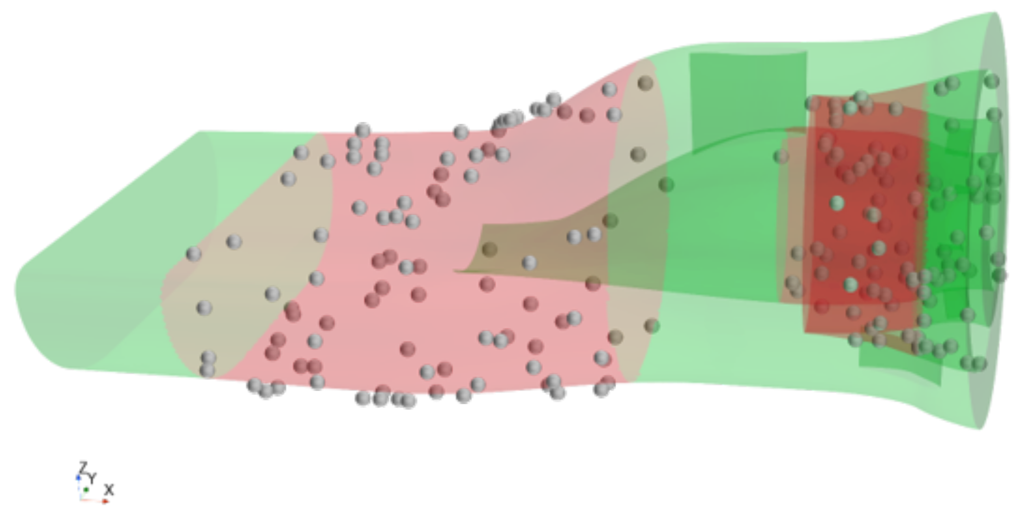
The first step of the adjoint optimization method consisted in determining the control points and the surfaces to be deformed. In order to ensure some stability in the process, as the adjoint method is really sensitive to the selection of the mobile surfaces, some simplifications were taken. Those parts that were close to the boundary conditions or to geometric limitations remained immobile and the adjoint did not act over them. Then, those mobile parts were fulfilled with control points whose coordinates served as inputs to the deformation function. The distance of the points with respect to the surface was adjusted by trial and error, but those trials were not included in the present paper due to their lack of interest, as they led to nonsensical geometries. In Figure 10, the mixer is divided in fixed parts, shown in green, and in mobile parts, shown in red. The control points and their initial position are also included, reflecting their chaotic distribution.

For the deformation function, a first-order gradient descent was proposed. This ordinary approximation permitted to compute the new position of the control points by evaluating the deformation function from the cumulative deformation and the new position of the control points scaled by a relaxation factor. This factor should be positive, as the optimization process minimized the cost function:

$$F_{\delta }=F_{\Delta }-5·{10}^{-6}·r_{points}$$

(10)

4.4.3. Cost Function

Once the control points and the deformation function were implemented, the next step was the definition of the cost function to be optimized. Traditionally, the adjoint optimization processes are focused on one single parameter. Nevertheless, the high restrictions derived from the correct performance of the compressor generated the need to consider other main variables whose evolution may be inversely proportional to the pressure drop optimization. Because of that, in the present paper, an algorithm is proposed where a specific weight is imposed to each one of the main variables. By modifying this weight, the limits of the range in which each variable can oscillate are set.

Starting from the values coming from the 2D optimization in its 3D configuration, after setting the objective value of each variable, the relative weight of each of them was imposed with respect to the main variable, defined as the total pressure at the outlet. In

Table 3. Weights of the cost function.

Variable	Weight	Obj. Value	$\mathbf{\Delta }$Variable	$\mathbf{\Delta }$Pressure
$\mathit{BPR}(-)$	1120	2.66	0.1	0.3
$\dot{\mathit{m}}$(kg/s)	130	5.92	0.1	0.5
${\mathit{UI}}_{\mathit{u}}(-)$	3224	1	0.1	0.1

, the weights and the possible variations are summarized. As it can also be observed in Table 3, a change of $10\%$ of the mass flow must imply a reduction in the pressure drop of $50\%$ to be worth it, due to the high restrictions in the nominal value of the mass flow used in the controller of the outlet, as defined in Section 3.3, whereas another value such as the uniformity index (UI), defined in Equation (13), which apparently is less restrictive in the context of achieving nominal points, did not present such resistances to the changes. The bypass ratio, defined before in Section 3.4 was also controlled, in order to ensure as much as possible our hypotheses were satisfied.

$$\begin{array}{c}\hfill \Delta P_t=P_{t,inlet,mixer}-P_{t,outlet,mixer}=\frac{P_{t,inlet,core}·{\dot{m}}_{core}+P_{t,inlet,bypass}·{\dot{m}}_{bypass}}{{\dot{m}}_{total}}-P_{t,outlet,mixer}\end{array}$$

(11)

$$F_{cost}=\Delta P_t+K_{BPR}·{(BPR-BP{R}_{obj})}^2+K_{UI}·{(U{I}_u-U{I}_{u,obj})}^2+K_{\dot{m}}·{(\dot{m}-{\dot{m}}_{obj})}^2$$

(12)

being

$$U{I}_u=1-\frac{{\sum }_f^n\left|u_f-\overline{u}\right|A_f}{2\left|u\right|{\sum }_f^n{A}_f}$$

(13)

5. Results

5.1. 2D Optimization Evaluation

Once the method was established, the next logical step was its implementation. As was indicated in Section 4.3.1, 64 total cases were evaluated.

Table 4. Tested variables and their levels.

Variable	Low	Medium	High	SN Signal
1	0.309	0.31	0.312	422.4307
2	0.065	0.07	0.075	420.655
3	0.14	0.15	0.16	1685.3
4	−0.115	−0.12	−0.125	1690
5	0.236	0.237	0.238	1271
6	−167	−168	−169	423.5
7	0.133	0.134	0.135	423.5
8	−0.29	−0.3	−0.31	421.4
9	0.206	0.207	0.208	2.89
10	0.18	0.19	0.2	423.5
11	0.24	0.25	0.26	421.4
12	−0.0525	−0.055	−0.0575	2.88
13	0.122	0.123	0.124	421.4

presents the different levels for each of the variables that constituted the design of experiments, as well as the influence of each of them on the solution according to the signal-to-noise ratio provided by the Taguchi method.

In

Table 5. Surface average results of the main variables.

Variable	2D Ini	2D Optim	Correspondent 3D
$\dot{\mathit{m}}(\mathbf{kg}/\mathbf{s}·\mathbf{rad})$	0.942	0.944	0.94
$\mathit{BPR}(-)$	3.49	2.64	2.66
${\mathbf{\Delta }}_{\mathit{p}}$(Pa)	270	229	229
${\mathit{UI}}_{\mathit{u}}(-)$	0.93	0.96	0.98
${\mathit{MI}}_{\mathit{\varphi }}(-)$	0.0311	0.0309	0.0310

, the variable combinations that resulted in the minimum pressure drop, along with other relevant results can be seen: the BPR, which can be proved to be within reasonable limits that would not compromise the main hypothesis; the mass flow per unit of angle, with which the mass controller at the outlet is checked; the UI of the velocity, whose high number provides a great index of the performance of the mixer, as it is means that the mixing performed as it should. Moreover, the table also includes a column where the values in the correspondent 3D case are shown, in order to verify that the hypothesis of axisymmetric flow in that part of the geometry was accomplished. It is also shown that the differences between the initial and the optimum case were remarkable, whereas the correspondent 3D values with respect to their homologous bidimensional values presented differences of barely $1\%$, while checking that neither the inclusion of the third component in the inlet velocity profiles nor the 3D solvers affected the solution in a determinant way.

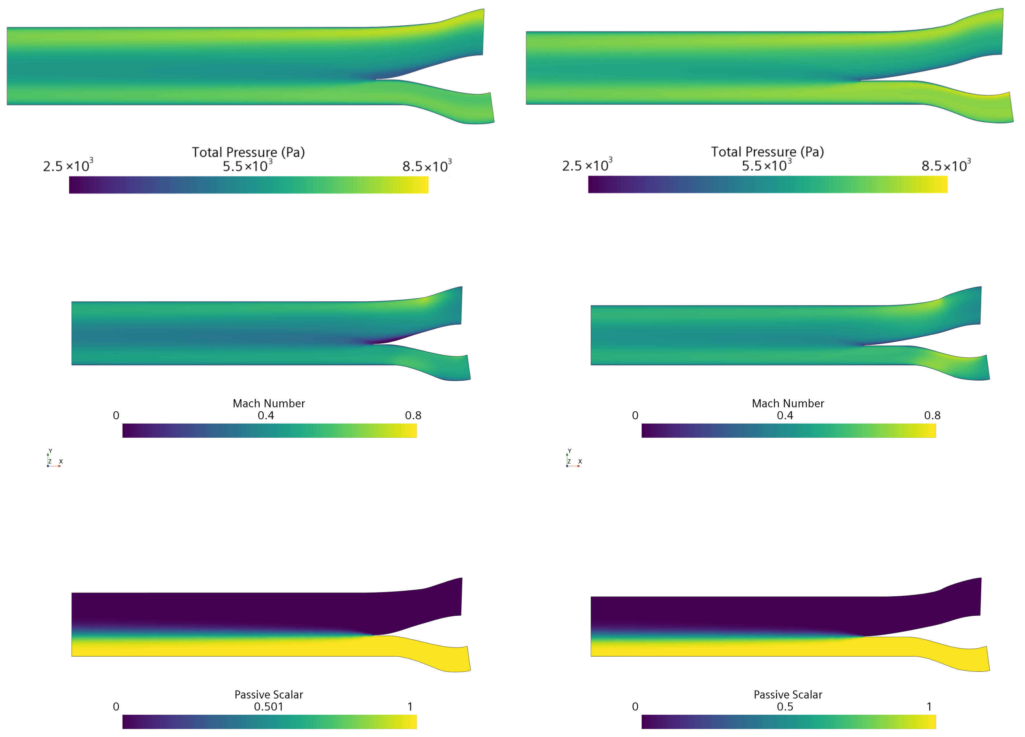
Together with the surface average parameters, the contours of the main scalar variables were compared with respect to the initial case. The Mach number and the total pressure contours are shown in Figure 11, in order to check the flow patterns and the quality of the mix. At a simple view it can be observed that the initial case presented an important detachment of the flow in the union of the streams, where there was definitely room for improvement. Moreover, in the outlet region, as a consequence of the heterogeneity of the flow, it can be observed that there were two main differenced jets of different pressures and velocities that compromised the mix. On the other hand, turning our attention to the optimized geometry, it is shown that the smoothness of the exterior faces, together with the new further position of the connecting point and the wider channel, helped the flow streamlines to follow the geometry itself, as well as arrived at the mixing channel with more homogeneous velocity values, as supported by the uniformity index. Finally, the mixing phenomena was also checked. Nevertheless, the horizontal characterization of the two branches prevented both streams from mixing, as can be seen in the passive scalar (represented by $\varphi$ in Equation (15)) patterns between zero and one where zero represented the flow coming from the bypass and one the flow coming from the core. According to related mixing studies [30], the mixing indexes at the outlet of the geometry presented extremely low and similar values for all cases, so it could not be used as a design criterion (see Table 5).

$$\begin{array}{c}\hfill M{I}_{\Phi ,new}=1-\frac{{\sum }_{i}d{A}_{unmixed-\Phi ,i}}{{\sum }_{i}d{A}_i}\end{array}$$

(14)

$$\begin{array}{c}\hfill d{A}_{unmixed-\Phi ,i}=\left\{\begin{array}{cc}\frac{{\varphi }_i-\overline{\varphi }}{(1-\overline{\varphi })+{\delta }_{\varphi ,new}}\hfill & \mathrm{if}\overline{\varphi }\le {\varphi }_i\le 1\hfill \\ \frac{\left|{\varphi }_i-\overline{\varphi }\right|}{(0-\overline{\varphi })+{\delta }_{\varphi ,new}}\hfill & \mathrm{if}0\le {\varphi }_i\le \overline{\varphi }\hfill \end{array}\right.\end{array}$$

(15)

5.2. 3D Optimization Evaluation

Once a 2D optimized design was found, and after the revolution and the addition of the second part of the whole mixer, the 3D optimization method was computed and evaluated.

Unlike in other methods, the changes derived from an adjoint method are really small between iterations, as it is constantly adjusting itself, so it is quite difficult to see them in a simple view. These changes are expected to be monotonous and asymptotic.

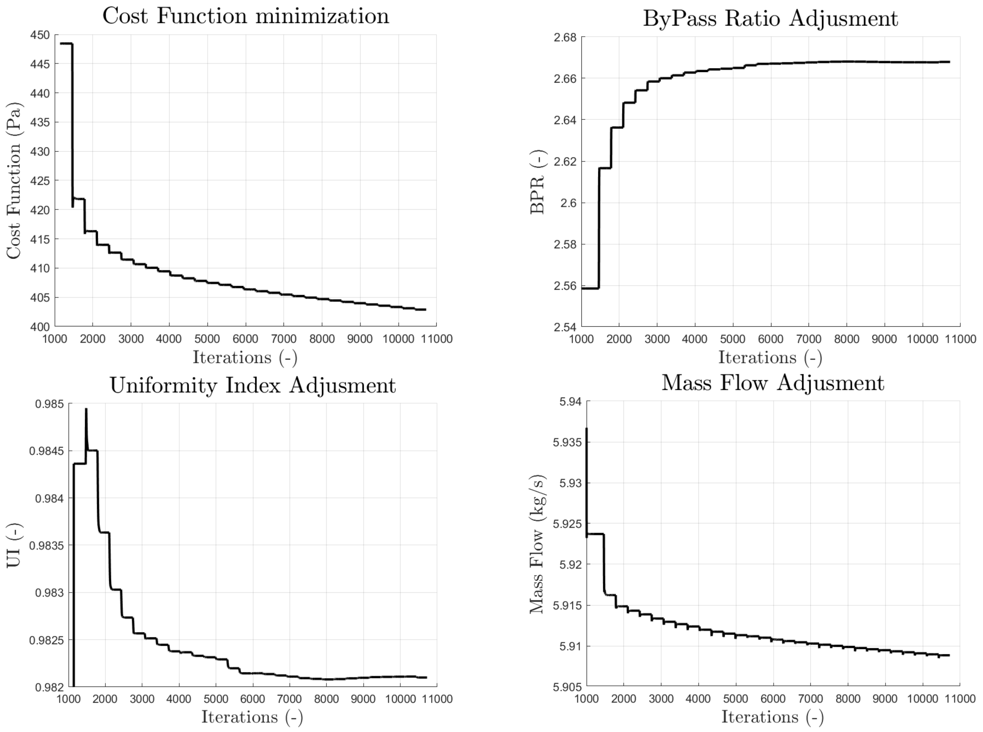
In Figure 12, the results of the cost function are summarized. The left top figure shows the minimization of the cost function itself. It is shown that the main correction was performed on the first iteration of the adjoint method, and after each iteration, the corrections were smaller than the previous one until the process converged to a final value.

The right top shows the evolution of the BPR. Like the cost function, the main change appeared in the first iteration and then it converged until the final value. It is worth mentioning that the BPR evolution, according to the objective value, was favourable to the study, because it reached the objective value at the same time as the cost function was minimized. On the other hand, by observing the UI and the mass flow of the case, the tendency was exactly the opposite. As the cost function decreased, both the UI and the mass flow moved away from the objective value. The UI decreased its value and so did the mass flow. Nevertheless, as the weight for each of the values was quite restrictive, the final mass flow and the objective mass flow differed by just $0.3\%$.

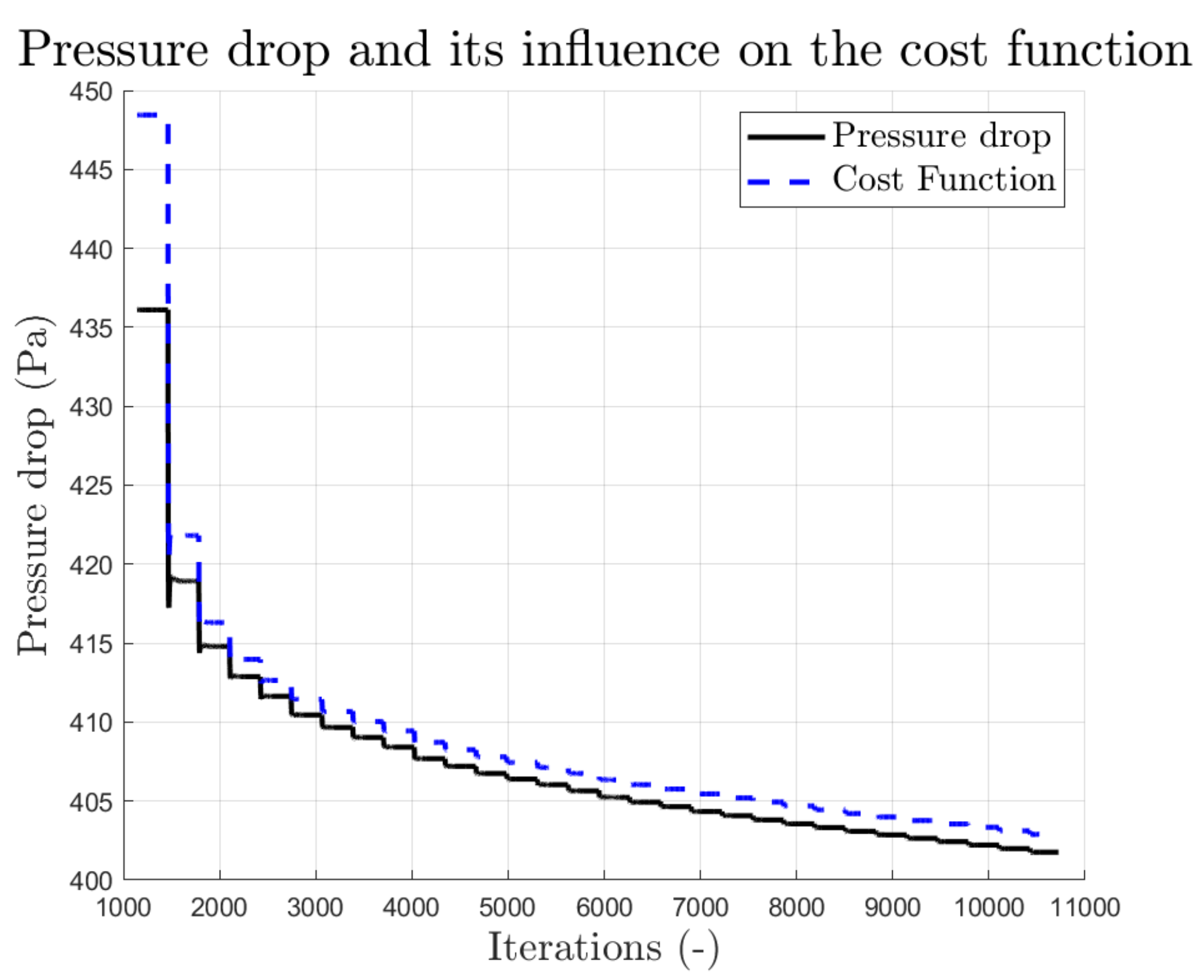
Once the cost function was analysed, the influence in the pressure drop had to be checked in order to see if the method worked. In Figure 13, the minimization of the pressure drop is shown and, following the same tendencies as those of the rest of the variables of the cost function, the value decreased (mainly in the first iterations) and converged to a final value of 402 Pa, which meant a decrease of approximately $10\%$ with respect to the initial value.

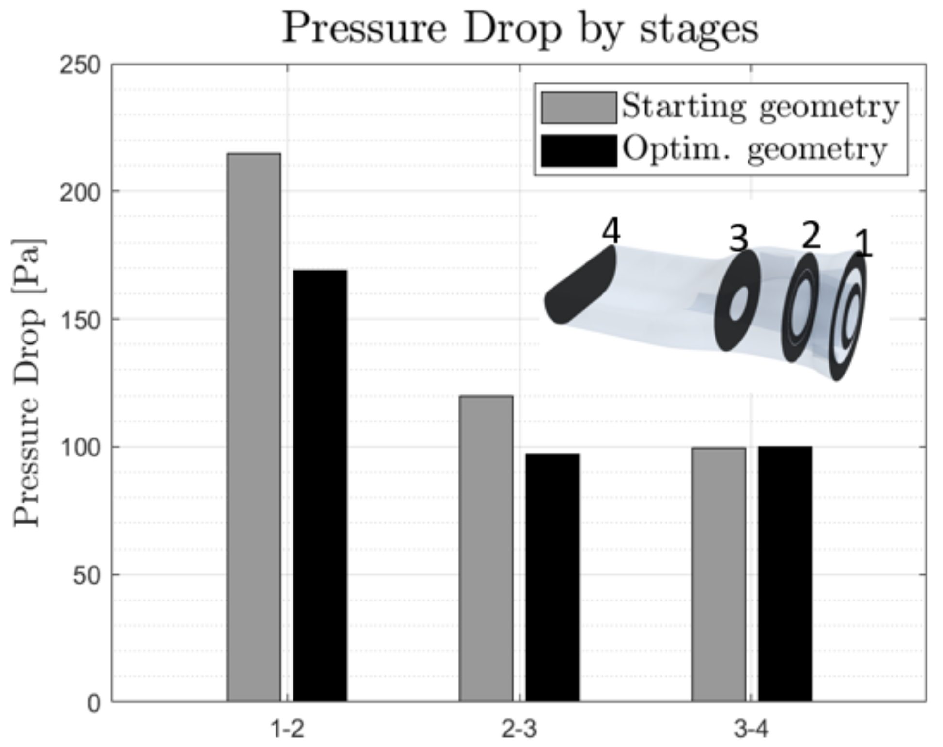
Together with the evaluation of the method, an analysis of the final geometry solution was conducted. As mentioned earlier, by analysing the differences of the main scalar contours between the original 3D geometry and the optimized one, no remarkable differences could be easily observed, although the pressure drop was minimized. In order to support the final results, an analysis of the total pressure stage by stage along the longitudinal axis of the mixer was performed, included in Figure 14, observing that the decrease in the pressure drop was mainly developed around the initial body of the mixer, where the main parts eligible for their optimization were defined, whereas in the bottom part, as already concluded, the solution was almost perfect, and no remarkable differences were observed.

Together with the averaged values, the velocity contours are included in Figure 15 in order to check the mentioned differences. Nevertheless, the nature of the adjoint method, which acts by only changing small details of the geometry, and the already well-designed mixer, which leads to small changes in the values, resulted in velocity contours where the differences were almost not noticeable.

5.3. Coupling Compressor and Mixer

Finally, once the optimization of the independent mixer was carried out, one last step was missing: the coupling of the compressor and the mixer. Moreover, a deeper analysis of the flow evolution was included since, being the ultimate case, it was clearly of interest. Having the averaged values of the main performance values of the compressor, the confirmation of the initial hypothesis had to be checked, so those values had to be compared, in order to assess the impact of the mixer design on shifting the compressor and mixer’s working point.

Table 6. Flow conditions at the interface between the compressor and the mixer.

Variable	Compressor Outlet BC	Compressor + Mixer	Difference (%)
$\dot{\mathit{m}}$(kg/s)	5.92	5.92	0
${\dot{\mathit{m}}}_{\mathit{core}}$(kg/s)	4.3	4.25	1.3
${\dot{\mathit{m}}}_{\mathit{bypass}}$(kg/s)	1.61	1.66	4
$\mathit{BPR}(-)$	2.67	2.55	4.5
${\mathit{P}}_{\mathit{t},\mathit{out}}$(Pa)	16,635	16,504	1
${\mathit{P}}_{\mathit{st},\mathit{out}}$(Pa)	13,400	13,200	1.5
${\mathit{P}}_{\mathit{t},\mathit{core}}$(Pa)	17,713	17,200	2.9
${\mathit{P}}_{\mathit{t},\mathit{bypass}}$(Pa)	17,104	16,649	2.6
${\mathbf{\pi }}_{\mathit{core}}(-)$	1.47	1.43	2.7
${\mathbf{\pi }}_{\mathit{bypass}}(-)$	1.42	1.385	2.3
${\mathit{T}}_{\mathit{t},\mathit{out}}$(K)	328	327	0.3
${\mathit{T}}_{\mathit{t},\mathit{core}}$(K)	328	327	0.3
${\mathit{T}}_{\mathit{t},\mathit{bypass}}$(K)	329	327	0.5
${\mathbf{\eta }}_{\mathit{core}}(-)$	0.84	0.8	3.5
${\mathbf{\eta }}_{\mathit{bypass}}(-)$	0.74	0.72	1.35

summarises some of the main results in the mixer and in the interface between the compressor and the mixer, as it is the most sensitive part which gives information about the strength of the taken hypothesis. By analysing the obtained data, it can be seen that differences of around $3\%$ and a maximum of $4.5\%$ were found between the simulation of the isolated mixer and the complete geometry, thus backing up quite strongly the adopted hypothesis and, in consequence, the proposed method of independent mixer optimization using a multidimensional approach.

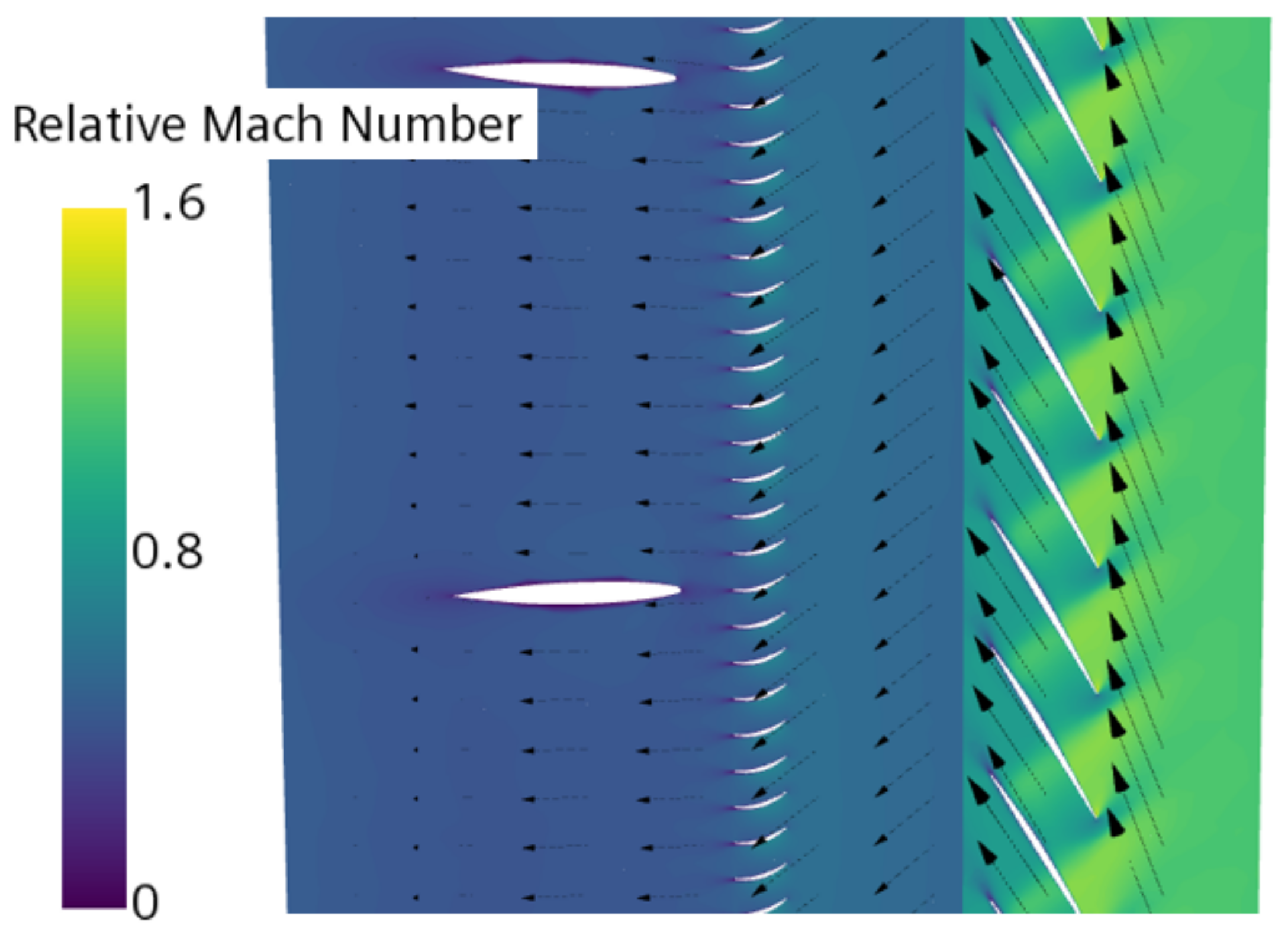
It was also interesting to check the correct behaviour of the compressor. For that, as mentioned before, the simulated point being a design point, the stream vectors corresponding to the flow at the rotor and stator blades are shown in Figure 16; we observe that the incidence of the flow was slightly positive but very close to zero. Moreover, the relative Mach contours confirmed the correct behaviour of the channels, as the incipient shock waves did not block them.

6. Concluding Remarks and Future Work

After developing the method and discussing the results, some relevant conclusions were obtained.

After justifying the need to adapt an existing compressor for such a new application both with the literature and with a numerical proof, a multidimensional optimization was developed by combining different strategies in a sequential process in order to include for the first time the mixer to the compressor element in the propulsive system of a hyperloop system. As it was conducted through the whole paper, minimizing the pressure drop of the mixer was the main objective, with the goal of achieving the highest pressure at the outlet in order to, in the subsequent stages of the propulsive system, such as the nozzle that returns the flow to the tube, reduce the aerodynamic losses. A first preliminary mixer was proposed based on a 0D analysis at the outlet of the compressor. After several different approximations, a custom function that took into account all of the approximations was chosen, achieving the second lowest difference of pressure between the branches of all the options, a reasonable low difference in velocities and the lowest outlet area, which could help achieve a smaller mixer that, in the end, would imply a lesser cost.

With this design as a guide, a 2D optimization of the axisymmetric parts with a remarkably low computational effort was performed, achieving a pressure drop reduction of $16\%$ with respect to the initial geometry. Moreover, the Taguchi analysis allowed us to identify those geometrical parameters that had no impact on the solution, opening the door for an iterative optimization method where those variables were not used. With the 3D optimization, although the method presented some difficulties in terms of selecting which surfaces were good candidates to be deformed, a conservative choice of the procedure was proposed and an additional $10\%$ in the minimization of the pressure drop was obtained. Hence, looking at these numbers, the idea of performing a first stage with an axisymmetric simplification turned out to be profitable, as a pressure drop improvement of $60\%$ was achieved in this process.

Finally, the evaluation of the main hypothesis was implemented, observing that there was a maximum deviation in the bypass ratio of $4.5\%$, whereas the rest of the flow variables just differed in values by around $1.5\%$. Nevertheless, the main limitation was due to the fact that the bypass ratio was constrained in order to match the operational design point of the compressor, so potential better solutions in terms of pressure drop may not have been taken into account. One possible solution would be the development of a method where the compressor was included during the whole process; however, this would lead to mesh domains 75 times bigger than the mixer alone, increasing in a considerable way the computational cost.

References

1. Eurostat; Commission Européenne. Energy, Transport and Environment Indicators; Office for Official Publications of the European Communities: Luxembourg, 2011; Volume 2. [Google Scholar]
2. Galindo, J.; Ruiz, S.; Dolz, V.; Royo-Pascual, L.; Haller, R.; Nicolas, B.; Glavatskaya, Y. Experimental and thermodynamic analysis of a bottoming Organic Rankine Cycle (ORC) of gasoline engine using swash-plate expander. Energy Convers. Manag. 2015, 103, 519–532. [Google Scholar] [CrossRef]
3. Friedlingstein, P.; Andrew, R.M.; Rogelj, J.; Peters, G.P.; Canadell, J.G.; Knutti, R.; Luderer, G.; Raupach, M.R.; Schaeffer, M.; van Vuuren, D.P.; et al. Persistent growth of CO2 emissions and implications for reaching climate targets. Nat. Geosci. 2014, 7, 709–715. [Google Scholar] [CrossRef]
4. Kumar, P. 4.02–Current and Future Perspectives on Hydrogen and Fuelcells for Its Potential Application in Portable, Stationary and Transportation Sectors. In Comprehensive Renewable Energy, 2nd ed.; Letcher, T.M., Ed.; Elsevier: Oxford, UK, 2022; pp. 29–54. [Google Scholar] [CrossRef]
5. Musk, E. Hyperloop Alpha; SpaceX: Hawthorne, CA, USA, 2013. [Google Scholar]
6. Goddard, E. Vacuum Tube Transportation System. U.S. Patent US2511979A, 20 June 1950. [Google Scholar]
7. Decker, K.; Chin, J.; Peng, A.; Summers, C.; Nguyen, G.; Oberlander, A.; Sakib, G.; Sharifrazi, N.; Heath, C.; Gray, J.S.; et al. Conceptual Feasibility Study of the Hyperloop Vehicle for Next-Generation Transport; Technical Report; American Institute of Aeronautics and Astronautics: Reston, VA, USA, 2017. [Google Scholar]
8. Sui, Y.; Niu, J.; Yu, Q.; Cao, X.; Yang, X. Numerical analysis of the aerothermodynamic behavior of a Hyperloop in choked flow. Energy 2021, 237, 121427. [Google Scholar] [CrossRef]
9. Nyanya, M.N.; Vu, H.B.; Schönborn, A.; Ölçer, A.I. Wind and solar assisted ship propulsion optimisation and its application to a bulk carrier. Sustain. Energy Technol. Assess. 2021, 47, 101397. [Google Scholar] [CrossRef]
10. Choi, S.Y.; Lee, C.Y.; Jo, J.M.; Choe, J.H.; Oh, Y.J.; Lee, K.S.; Lim, J.Y. Sub-Sonic Linear Synchronous Motors Using Superconducting Magnets for the Hyperloop. Energies 2019, 12, 4611. [Google Scholar] [CrossRef] [Green Version]
11. Pradhan, R.; Katyayan, A. Vehicle dynamics of permanent-magnet levitation based Hyperloop capsules. In Proceedings of the ASME 2018 Dynamic Systems and Control Conference, Atlanta, GA, USA, 30 September–3 October 2018; Volume 51906, p. V002T22A004. [Google Scholar]
12. Rana, Y. On the Feasibility of the Hyperloop Concept. Ph.D. Thesis, Massachusetts Institute of Technology, Cambridge, MA, USA, 2020. [Google Scholar]
13. Kantrowitz, A.; Donaldson, C.D. Preliminary Investigation of Supersonic Diffusers; Technical Report; NASA: Langley Field, VA, USA, 1945. [Google Scholar]
14. Nalivaychenko, D. Analysis of the issues of Kantrowitz limit passing by the body, gradually accelerating up to the supersonic speed in the axisymmetric channel. AIP Conf. Proc. 2019, 2125, 030022. [Google Scholar]
15. Lluesma-Rodríguez, F.; González, T.; Hoyas, S. CFD simulation of a hyperloop capsule inside a closed environment. Results Eng. 2021, 9, 100196. [Google Scholar] [CrossRef]
16. Bose, A.; Viswanathan, V. Mitigating the Piston Effect in High-Speed Hyperloop Transportation: A Study on the Use of Aerofoils. Energies 2021, 14, 464. [Google Scholar] [CrossRef]
17. Opgenoord, M.M.; Caplan, P.C. Aerodynamic design of the Hyperloop concept. AIAA J. 2018, 56, 4261–4270. [Google Scholar] [CrossRef]
18. Braun, J.; Sousa, J.; Pekardan, C. Aerodynamic design and analysis of the hyperloop. AIAA J. 2017, 55, 4053–4060. [Google Scholar] [CrossRef]
19. Le, T.T.G.; Kim, J.; Cho, M.; Ryu, J. Effects of tail shapes/lengths of Hyperloop pod on aerodynamic characteristics and wave phenomenon. Aerosp. Sci. Technol. 2022, 131, 107962. [Google Scholar] [CrossRef]
20. Bizzozero, M.; Sato, Y.; Sayed, M.A. Aerodynamic study of a Hyperloop pod equipped with compressor to overcome the Kantrowitz limit. J. Wind Eng. Ind. Aerodyn. 2021, 218, 104784. [Google Scholar] [CrossRef]
21. Hong, S.; Kang, H.; Kwon, H. Development of compressor performance analysis module for Capsule Train CFD analysis. KSFM J. Fluid Mach. 2019, 22, 28–34. [Google Scholar] [CrossRef]
22. Lluesma-Rodríguez, F.; González, T.; Hoyas, S. CFD Simulation of a Hyperloop Capsule Inside a Low-Pressure Environment Using an Aerodynamic Compressor as Propulsion and Drag Reduction Method. Appl. Sci. 2021, 11, 3934. [Google Scholar] [CrossRef]
23. Zhou, K.; Ding, G.; Wang, Y.; Niu, J. Aeroheating and aerodynamic performance of a transonic hyperloop pod with radial gap and axial channel: A contrastive study. J. Wind Eng. Ind. Aerodyn. 2021, 212, 104591. [Google Scholar] [CrossRef]
24. Janke, C.; Bestle, D.; Becker, B. Compressor map computation based on 3D CFD analysis. CEAS Aeronaut. J. 2015, 6, 515–527. [Google Scholar] [CrossRef]
25. Karniadakis, G.; Beskok, A.; Aluru, N. Microflows and Nanoflows: Fundamentals and Simulation; Springer: Cham, Switzerland, 2006; Volume 29. [Google Scholar]
26. Large-Scale DES Analysis of Stall Inception Process in a Multi-Stage Axial Flow Compressor. In Proceedings of the ASME Turbo Expo 2016: Turbomachinery Technical Conference and Exposition, Seoul, South Korea, 13–17 June 2016; p. V02DT44A021. [CrossRef]
27. Menter, F. Zonal Two Equation k-w Turbulence Models For Aerodynamic Flows. In Proceedings of the 23rd Fluid Dynamics, Plasmadynamics, and Lasers Conference, Orlando, FL, USA, 6–9 July 1993. [Google Scholar] [CrossRef]
28. Ayesha Khan, M.; Arunagiri, P.; Antony Samuel Prabu, G. Parametric investigation on a transonic axial compressor stage using CFD techniques. Mater. Today Proc. 2020, 33, 912–918. [Google Scholar] [CrossRef]
29. Burberi, C.; Michelassi, V.; Scotti del Greco, A.; Lorusso, S.; Tapinassi, L.; Marconcini, M.; Pacciani, R. Validation of steady and unsteady CFD strategies in the design of axial compressors for gas turbine engines. Aerosp. Sci. Technol. 2020, 107, 106307. [Google Scholar] [CrossRef]
30. Galindo, J.; Gil, A.; Navarro, R.; García-Olivas, G. Numerical assessment of mixing of humid air streams in three-way junctions and impact on volume condensation. Appl. Therm. Eng. 2022, 201, 117676. [Google Scholar] [CrossRef]
31. Karim, A.; Mckean, M.; Dehner, R.; Selamet, A.; Tiernan, C.; Morelli, A.; Miazgowicz, K.; Mull, T. Turbocharger Centrifugal Compressor Casing Treatment for Improved BPF Noise Using Computational Fluid Dynamics. SAE Int. J. Adv. Curr. Pract.-Mobil. 2019, 128, 99EJ. [Google Scholar] [CrossRef]
32. Broatch, A.; Galindo, J.; Navarro, R.; García-Tíscar, J. Numerical and experimental analysis of automotive turbocharger compressor aeroacoustics at different operating conditions. Int. J. Heat Fluid Flow 2016, 61, 245–255. [Google Scholar] [CrossRef] [Green Version]
33. Tüchler, S.; Chen, Z.; Copeland, C.D. Multipoint shape optimisation of an automotive radial compressor using a coupled computational fluid dynamics and genetic algorithm approach. Energy 2018, 165, 543–561. [Google Scholar] [CrossRef]
34. Neverov, V.; Kozhukhov, Y.; Yablokov, A.; Lebedev, A. Optimization of a centrifugal compressor impeller using CFD: The choice of simulation model parameters. IOP Conf. Ser. Mater. Sci. Eng. 2017, 232, 012037. [Google Scholar] [CrossRef]
35. Cornelius, C.; Biesinger, T.; Galpin, P.; Braune, A. Experimental and Computational Analysis of a Multistage Axial Compressor Including Stall Prediction by Steady and Transient CFD Methods. J. Turbomach. 2013, 136, 061013. [Google Scholar] [CrossRef]
36. Capetillo, A.; Ibarra, F. Multiphase injector modelling for automotive SCR systems: A full factorial design of experiment and optimization. Comput. Math. Appl. 2017, 74, 188–200. [Google Scholar] [CrossRef]
37. Immonen, E. CFD optimization of jet fan ventilation in a car park by fractional factorial designs and response surface methodology. Build. Simul. 2015, 9, 1–9. [Google Scholar] [CrossRef]
38. Seenivasan, V.; Sakthivel, M.; Sudhagar, S.; Daniel, A. Modification of the cyclone separator geometry for improving the performance using Taguchi and CFD approach. Part. Sci. Technol. 2018, 37, 1–10. [Google Scholar] [CrossRef]
39. Wang, Z.; Wang, Y.; Zhuang, M. Improvement of the aerodynamic performance of vertical axis wind turbines with leading-edge serrations and helical blades using CFD and Taguchi method. Energy Convers. Manag. 2018, 177, 107–121. [Google Scholar] [CrossRef]
40. Rößger, P.; Richter, A. Performance of different optimization concepts for reactive flow systems based on combined CFD and response surface methods. Comput. Chem. Eng. 2018, 108, 232–239. [Google Scholar] [CrossRef]
41. Taguchi, G. Introduction to Quality Engineering: Designing Quality into Products and Processes; Technical Report; Wiley: Hoboken, NJ, USA, 1986. [Google Scholar]
42. Rosa, J.; Robin, A.; Silva, M.; Baldan, C.; Peres, M. Electrodeposition of copper on titanium wires: Taguchi experimental design approach. J. Mater. Process. Technol. 2009, 209, 1181–1188. [Google Scholar] [CrossRef]
43. Cea, J. Conception optimale ou identification de formes, calcul rapide de la dérivée directionnelle de la fonction coût. ESAIM Math. Model. Numer. Anal. 1986, 20, 371–402. [Google Scholar] [CrossRef] [Green Version]
44. Clare, M.C.; Kramer, S.C.; Cotter, C.J.; Piggott, M.D. Calibration, inversion and sensitivity analysis for hydro-morphodynamic models through the application of adjoint methods. Comput. Geosci. 2022, 163, 105104. [Google Scholar] [CrossRef]
45. Cockburn, B.; Xia, S. An adjoint-based adaptive error approximation of functionals by the hybridizable discontinuous Galerkin method for second-order elliptic equations. J. Comput. Phys. 2022, 457, 111078. [Google Scholar] [CrossRef]
46. Broatch, A.; Olmeda, P.; García-Tíscar, J.; Felgueroso, A.; Chávez-Modena, M.; González, L.; Gelain, M.; Couilleaux, A. Experimental aerothermal characterization of surface air-cooled oil coolers for turbofan engines. Int. J. Heat Mass Transf. 2022, 190, 122775. [Google Scholar] [CrossRef]
47. Li, M.; Chen, J.; Feng, X.; Qu, F.; Bai, J. An efficient adjoint method for the aero-stealth shape optimization design. Aerosp. Sci. Technol. 2021, 118, 107017. [Google Scholar] [CrossRef]
48. Spalart, P.; Allmaras, S. A One-Equation Turbulence Model for Aerodynamic Flows. In Proceedings of the 30th Aerospace Sciences Meeting and Exhibit, Reno, NV, USA, 6–9 January 1992. [Google Scholar] [CrossRef]
49. Saad, Y.; Schultz, M.H. GMRES: A Generalized Minimal Residual Algorithm for Solving Nonsymmetric Linear Systems. SIAM J. Sci. Stat. Comput. 1986, 7, 856–869. [Google Scholar] [CrossRef] [Green Version]
50. Anderson, M.R. Comprehensive Smith Charts for Axial Compressor Design. In Proceedings of the ASME Turbo Expo 2019: Turbomachinery Technical Conference and Exposition, Phoenix, AZ, USA, 17–21 June 2019. [Google Scholar] [CrossRef]
51. Cordier, O. Ähnlichkeitsbedingungen für Strömungsmaschinen. BWK BD 1953, 6, 337–340. [Google Scholar]
Figure 1. Conceptual model of the complete pod with a frontal compressor.
Applsci 12 12795 g001
Figure 2. Geometry of the compressor and the mixer.
Applsci 12 12795 g002
Figure 3. Flux diagram of the uncoupled process In square, the methodology steps. In oval, the results of the optimization stages.
Applsci 12 12795 g003
Figure 4. Global external surface reference mesh (75M elements).
Applsci 12 12795 g004
Figure 5. Mesh details at the leading edge of the rotor (reference mesh of 75M elements).
Applsci 12 12795 g005
Figure 6. 2D mesh. The dashed red line marks the end of the axisymmetric body in the original geometry.
Applsci 12 12795 g006
Figure 7. Evaluation of the different tested methods in terms of area, pressure and velocity.
Applsci 12 12795 g007aApplsci 12 12795 g007b
Figure 8. Control variables of the Taguchi optimization method.
Applsci 12 12795 g008
Figure 9. Flowchart of the implemented adjoint method.
Applsci 12 12795 g009
Figure 10. Control points of the adjoint method.
Applsci 12 12795 g010
Figure 11. Flow field comparison between the initial (left) and the optimum (right) cases.
Applsci 12 12795 g011
Figure 12. Cost function evaluation.
Applsci 12 12795 g012
Figure 13. Pressure drop minimization.
Applsci 12 12795 g013
Figure 14. Pressure drop by stages along the x axis in the mixer.
Applsci 12 12795 g014
Figure 15. Velocity patterns comparison between initial (left) and final (right) 3D geometries. The top cut is given by the intersection of the geometry and the plane Z = −0.5. The bottom cut is given by the intersection of the geometry and the plane Y = 0 (symmetry plane).
Applsci 12 12795 g015
Figure 16. Relative velocity contours and vectors in a rotor and stator channel.
Applsci 12 12795 g016