Coastal Flooding Assessment Induced by Barometric Pressure, Wind-Generated Waves and Tidal-Induced Oscillations: Kaštela Bay Real-Time Early Warning System Mobile Application

Abstract

Our work presents a reliable procedure to obtain real-time assessment of the sea water elevation at the Kaštela Bay site to ensure the a priori warning in the case of expected coastal flooding along the site area. In its origin, the presented procedure relies on relevant data sets which are site-specific and locally observed. Observed data sets are used within the procedure to assess sea water surface elevation when induced by barometric pressure changes and wind-generated waves. Tidal-induced changes are introduced into the assessment procedure by a pre-learned algorithm which relies on long-term sea level oscillations from the relevant tidal gauge. Wind-generated wave heights are determined in the near shore area, following the features of the depth and reflection of the shoreline subsections. By coupling three mechanisms, this paper offers a unique real-time procedure to determine the sea water elevation and assess the possibility for coastline structure to be flooded by the sea. Given information is visualized in a form of mobile application that implements the algorithm and allows end users to set the notifications based on the given ruleset.

1. Introduction

Coastal flooding events, including their occurrence and triggers for the appearance of waves, have been investigated in the past to contribute to a better understanding of flood events in coastal areas as well as efficient risk management. Recent investigations have studied the occurrence of storm and sea wave events [1,2], the numerical modelling of wave propagation in coastal areas [3], flood water movement over land areas [4], the impact of storms on coasts [5] and flood vulnerability [6].

Special attention has been given to the development of an early warning system (EWS) for the timely warning of residents in exposed areas as well. Early warning systems are also an integral part of coastal flood management plans and contribute to the development of long-term management strategies [7]. Existing sea-state monitoring technology, historical databases, numerical forecasting models and computer science have been parts of the operational coastal flood early warning system [8]. A EWS modelling framework based on a Bayesian network has been used to link coastal hazards to their socio-economic and environmental factors [9] and connect available field measurements, data obtained from numerical wave simulations and an empirical wave run-up approach [10]. An EWS that determines the total sea level height by combining predictions of tides and sea level anomalies with wave runup estimates has been presented in [11].

Technological progress in computation and communication sciences in the last decade allows for work with large databases that can store registered meteorological data that affect the occurrence of sea floods. This type of data represents a basis for developing different forecasting platforms, which use input data and boundary conditions from global or regional scales and open sea and weather forecast databases, providing wave propagation in the ports [12]. These platforms use a number of effective hydrodynamic numerical models for the simulation of storm surge and the prediction of sea water level [13]. It is important to notice that the sea water level prediction procedure in real time is a time-consuming process which needs significant computational resources, as well as the development and monitoring of a software architecture [14] to model coupling and integration. The models based on machine learning [15] and artificial intelligence provide easy implementation of numerical models with low computational cost, as well as fast training, validation, testing and evaluation [16].

In the present study, coastal flooding caused by the simultaneous combination of several mechanisms, such as tidal-induced sea level oscillations resulting from barometric pressure changes and wind-generated waves, have been investigated in the Kaštela Bay. A special focus has been given to the area of the city of Kaštela, placed at the north part of the bay (Figure 1), with many cultural and historical buildings and/or areas located near the coastline, which are potentially endangered by coastal flooding and subject to significant consequences and damage (Figure 2).

The design of the early warning system for sea flooding risk in the city of Kaštela includes the following components:

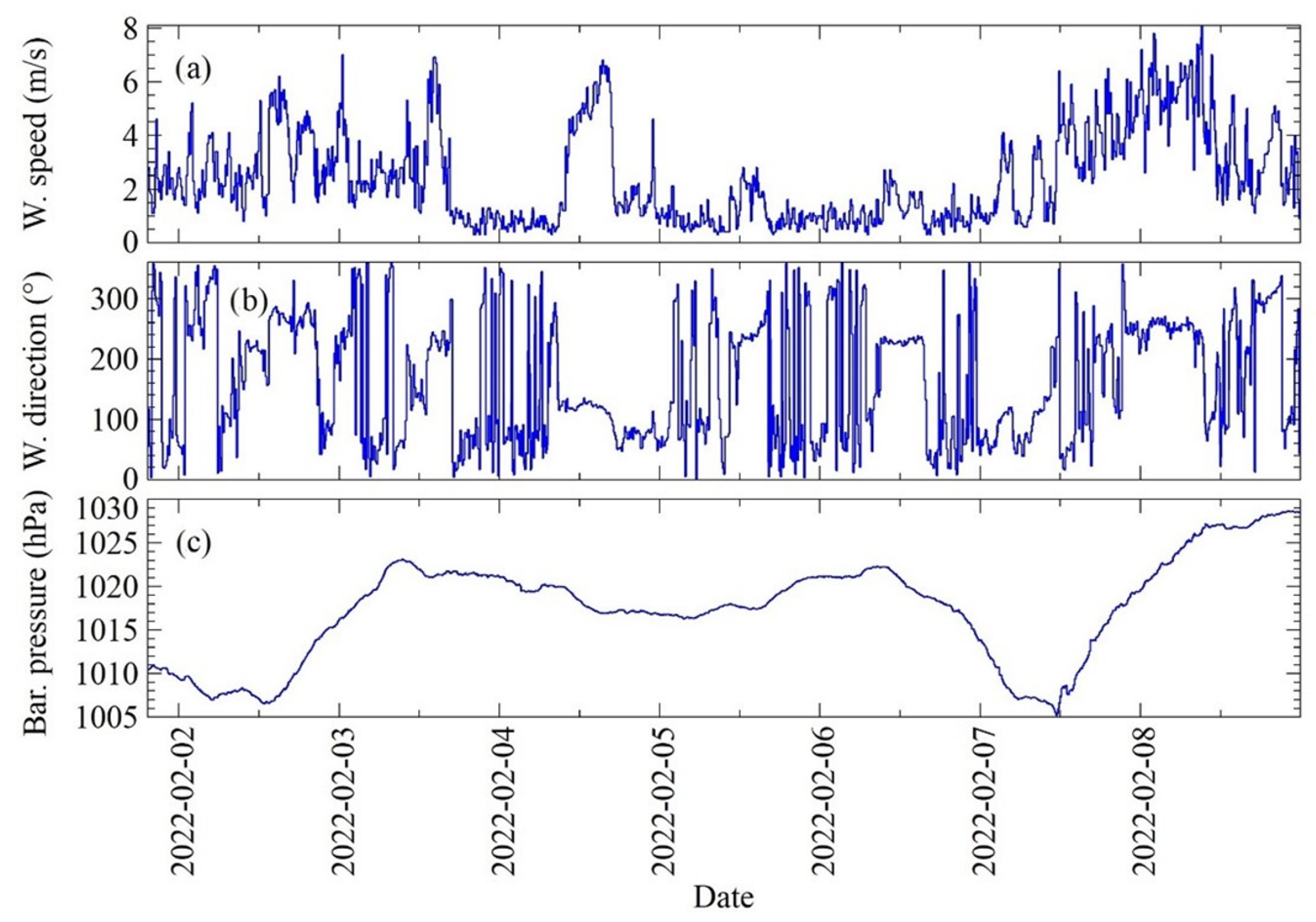
• A monitoring system consisting of an installation of hardware at the site location and appropriate software for real-time data collection. This system observes the wind speed and the barometric pressure.
• Application of mathematical and numerical models for sea level prediction on the coastline: Numerical model is used to analyze the wave transform mechanism. A specific procedure has been established to incorporate simultaneous effects of wind-generated waves, tides and barometric pressure-induced changes in the sea level to determine sea level at the coastline based on the systematic observations of the abovementioned parameters via a real-time monitoring system (wind speed and direction and barometric pressure). Tidal-induced sea level changes have been obtained based on the past observations of the long-term sea level tidal oscillations from the relevant tidal gauge.
• Estimation of the risk of flooding for humans: Using a digital terrain model where each pixel is georeferenced (X, Y coordinates) and assigned altitude Z, the calculated sea heights will be compared with the altitudes, and if the sea elevation is greater than the altitude Z of a pixel, that pixel will be marked as flooded. According to the depth of the sea on land, the risk of flooding for humans will be defined based on an analytical function so that it can be easily integrated into the rest of the system. This information is necessary for the input into the early warning system. For a simple and understandable presentation of the flooding risk, the analyzed coastal area is divided into zones in order to define the total sea level. This division is made according to the criteria of the coast type and the coast height, which have a direct impact on the height of the waves.
• Dissemination and communication of risk information by mobile application: Flood warnings will be given to people who have the mobile application, which was developed for the purpose of the dissemination of information about flood risk in the observed area. Those that have installed the application on their mobile phone and enabled that app to send them push notifications will receive the information.

Recently, Internet of Things (IoT) systems that monitor in different scenarios to ensure a green, sustainable future have been widely used to create smart environments tailored to particular human needs [17,18]. Affordable equipment, miniaturized in its deployment, is ensured a long lifetime through solar/battery power; the communication ranges are also extremely increased and can be measured in kilometers in urban areas, which is especially pertinent in meteorological scenarios [19,20]. In this study, the established sea level monitoring system uses an IoT-based, solar-powered anemometer (Barani design—Meteo Wind) and solar-powered meteo-station (Barani design Meteo-helix) for monitoring air pressure. The system is deployed to acquire current meteorological information used as an input for the developed model to estimate the sea level. The system is based on the LoRaWAN IoT radio, which delivers the information to The Things Network (TTN) cloud system, which is then used by the cross-platform web/mobile application called Waves, which is used as an early warning monitoring system. The multilanguage system itself implements: (1) the algorithm that defines sea level based on the tidal, wind speed/direction and air pressure information; (2) information on the shore height at the dedicated measurement and early warning zones; (3) push notification logics that can be separately activated based on user’s zone of the interest.

This paper presents a methodological approach for the development of an early warning system for coastal flooding. It is based on frequently measured meteorological data and sea level predictions integrated on a single platform to provide real-time information about potential risk for the citizens of the city of Kaštela.

Novelties of the manuscript are summarized as follows: (i) to our best knowledge, the site of the application has been used for the very first time to demonstrate the application of the coastal flooding early warning system; (ii) the relevance of the selected site relies on the fact that the area is faced with coastal flooding more than 15 days per year on average, thus increasing the need for early warning system development, (iii) the manuscript couples three mechanisms contributing to the coastal flooding vulnerability assessment, those being barometric pressure-induced sea level changes, wind-generated waves and tidal-induced fluctuations, (iv) barometric- and tidal-induced sea level changes are obtained in real time, fully relying on local conditions arising from the observations, (v) wind-generated wave heights are site specific, taking into consideration bathymetric features and coastal structure type and (vi) the whole procedure has been implemented in the form of a real-time mobile application, thus resulting in a reliable tool for the end users.

Compared to relevant publications [16,21], this paper couples three of the mechanisms leading to the sea water level rise and refers to a site-specific area. Although it does not offer general findings, the procedure shows the potential to be applied to other sites all over the Mediterranean basin after prior modifications. The latter refers to bathymetric features, the reflection of the coastline, the determination of incident deep water wave parameters and tidal observations.

The paper is structured as follows: Section 2 is the Methodology and Study area section, which couples the methodology used in the study with representative site related data. Section 3 offers Results from the study, while Section 4 consists of relevant Discussion topics and Section 5 summarizes main conclusion points.

2. Methodology and Site Description

2.1. Sea Water Elevation Prediction

Sea water level is a random process resulting from the simultaneous combination of several mechanisms, three of which are found to be dominant, those being tidal-induced oscillations and oscillations due to barometric pressure changes and wind-generated waves. Although characterized by different time scales, those three mechanisms simultaneously contribute to the absolute sea water elevation definition.

Tidal-induced sea water oscillations are driven by tidal forcing, which is induced by simultaneous inter gravity forces between the Sun, Moon and Earth. Tidal-induced changes are characterized as a mixed semidiurnal type at the location of interest, with main periodic intervals corresponding to both semi diurnal and diurnal ones. Compared to tidal oscillations, sea level changes induced by barometric pressure changes are aperiodic with time scales corresponding to two main factors: (i) daily barometric pressure changes corresponding to daily scale air temperature change and (ii) time scales corresponding to the time necessary for the air mass transfer from different geographic locations to the location of interest to occur. The latter corresponds to time scales usually equal to several hours. Wind-generated waves are characterized by very small time scales, up to 8 s in the area of interest, and these are generated as a result of the air mass kinematic energy transfer to the sea surface.

Previous research [22] has shown that tides characterizing the Adriatic Sea basin consist mainly of seven dominant constituents, of which three are diurnal (O1, P1 and K1) and four are semidiurnal (N2, M2, S2 and K2). In its origin, each constituent represents a sinusoidal function with an associated amplitude, period, and phase, contributing to the full tidal signal. To determine the unknown values of the amplitudes, periods and phases, the original signal is initially transferred from the time to frequency domain by applying the Discrete Fourier Transform (DFT) [22]. DFT results are often plotted as Amplitude Spectral Density (ASD). By normalizing magnitudes with number of samples, the amplitude of each frequency can be easily obtained. Due to the fact that DFT calculations are time demanding [23], Fast Fourier Transform (FFT) [24] incorporated in Python in SciPy library [23] has been used for faster transfer of signals from the time to frequency domain. Based on the determined tidal constituent parameters, the tidal-induced sea level can be simulated using a linear superposition of sine functions corresponding to the number of relevant constituents:

$$h_t={\displaystyle \sum }_{i=1}^7{A}_i\times \sin \left(\frac{2\pi t}{t_{pi}}+\frac{2\pi {\phi }_i}{360}\right), t=0, 1, \dots , M$$

(1)

where h_t is the simulated sea level [m], A_i is the amplitude [m], t_pi is the period [h] and φ_i phase [°] of i-th constituent, M is the sample size and t is relative time [h].

Simulated sea level h_sea can be calculated as a superposition of tidal harmonics from Equation (2) by adding the mean sea level value calculated from the observed sea level signal:

$$h_{sea}=h_t+\overline{h}$$

(2)

where h_t represents tidally induced sea level oscillations and $\overline{h}$ represents the mean sea level value.

Increasing the barometric pressure by 1 [cm] of the saltwater column leads to a decrease in the sea level by approximately 1 [cm] and inversely, decreasing the barometric pressure by 1 [cm] raises the sea level by 1 [cm] [25]. This effect is called the Invert Barometric effect (IB). The sea level rise caused by the change of the barometric pressure can be calculated as follows:

$$h_{at}=\frac{-p_a}{\rho g}$$

(3)

where h_at is the sea level change resulting from a change in barometric pressure, p_a is the barometric pressure [Pa] change, ρ is the density of sea water [kg/m³] and g is the gravitational acceleration [m/s²]. Therefore, the simulated sea level incorporating both tidal oscillations and barometric pressure-induced changes is updated from Equation (2) for the value of h_at, as shown in Equation (3):

$$h_{sea}=h_t+h_{at}+\overline{h}$$

(4)

where the third right hand term ($\overline{h}$) represents mean sea level values as calculated from the observed signal, h_t represents tidally induced sea level oscillations and h_at stands for barometric pressure-induced sea level change.

To assess wind-generated wave height in front of the coastline, we start with a determination of deep water wave parameters. For the location of interest and relevant incident wave directions, fetch length has been assessed by applying the Saville method [26]. In order to determine deep water wave parameter values, data sets from the Section 2.3 climatological station have been used. Fully developed sea conditions have been checked by applying the Wilson criteria [27] prior to the determination of wave parameters. After defining relevant fetch length for a given wind duration and wind velocity, the Groen−Dorrestein nomogram is used to determine deep water wave parameters [28].

Wave transform analysis has been performed by applying SMS CGWAVE software [29]. The wave phenomena that can be simulated by CGWAVE are: bathymetric refraction, diffraction by structures (e.g., breakwaters) and bathymetry, reflection (from structures, natural boundaries (seawalls, coastlines, etc.) and bed slopes), friction, wave breaking and floating (fixed) docks influence the wave field. The model is based on the use of a triangular finite element formulation to solve the two-dimensional elliptic mild slope equation, with grid sizes varying throughout the domain based on the local wavelength [30]. The grid can be efficiently generated using the SMS graphical interface when a bathymetry file is provided. The model allows one to specify the desired reflection properties along the coastline and other internal boundaries. While the basic equation is intended for monochromatic waves, irregular (i.e., spectral) wave conditions are simulated in CGWAVE through a linear superposition of monochromatic simulations [31,32].

The procedure or the algorithm for the absolute sea water elevation assessment is based on three steps which are presented above and summarized as: (i) sea level change caused by tidal forcing prediction, (ii) sea level change caused by a barotrophic pressure forcing assessment and (iii) assessment of the wind-generated wave height in front of the coastline. Sea water elevation assessment as a consequence of simultaneous effects for those three mechanisms is assessed as follows:

• From observed tidally induced oscillations, the harmonic parameters (amplitude, period and phase) are initially determined based on the Least Square Method application;
• After all harmonic parameters have been determined, tidal-induced sea level oscillation is determined by using Equation (1);
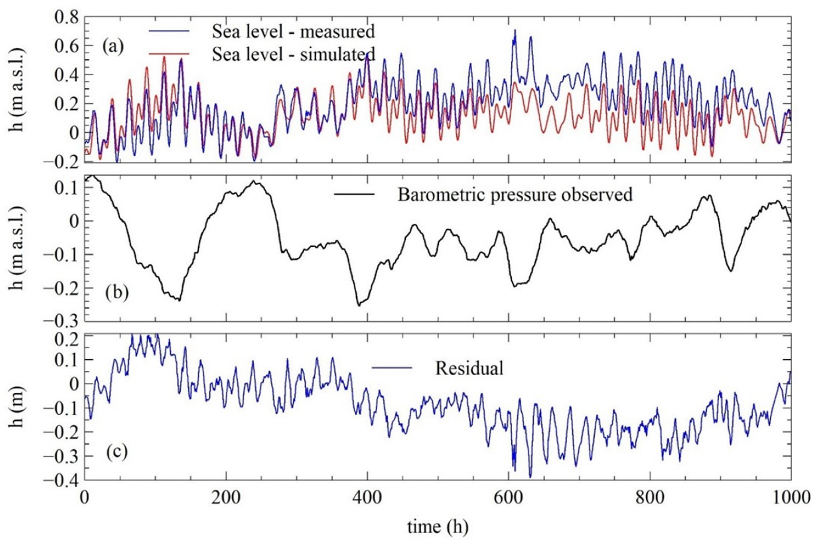
• From observed barometric pressure data, the change in sea level induced by the drop/rise of the barometric pressure is determined from Equation (3);
• Deep water wave parameters are determined depending on incident direction and wind velocity and duration parameters;
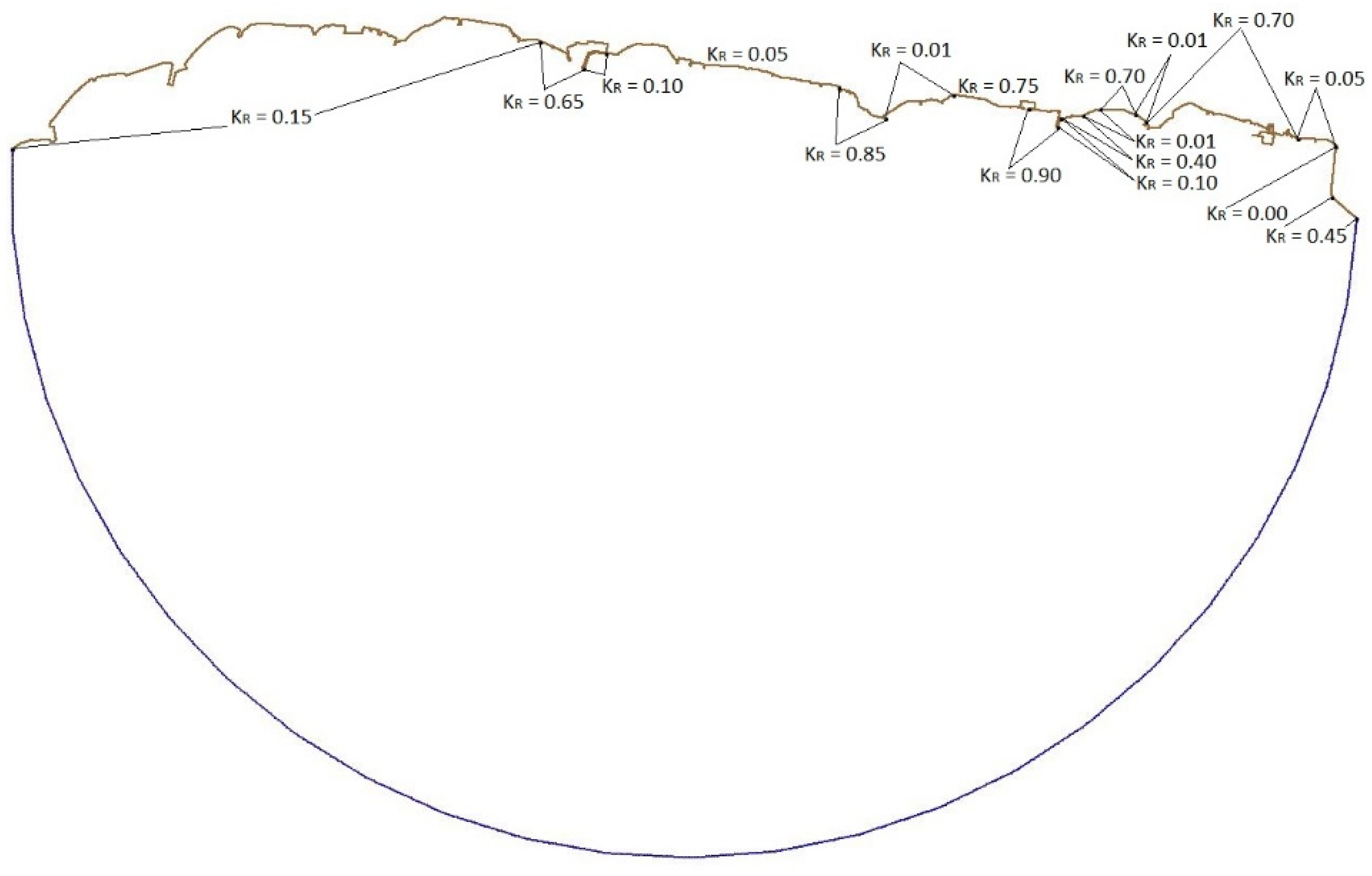
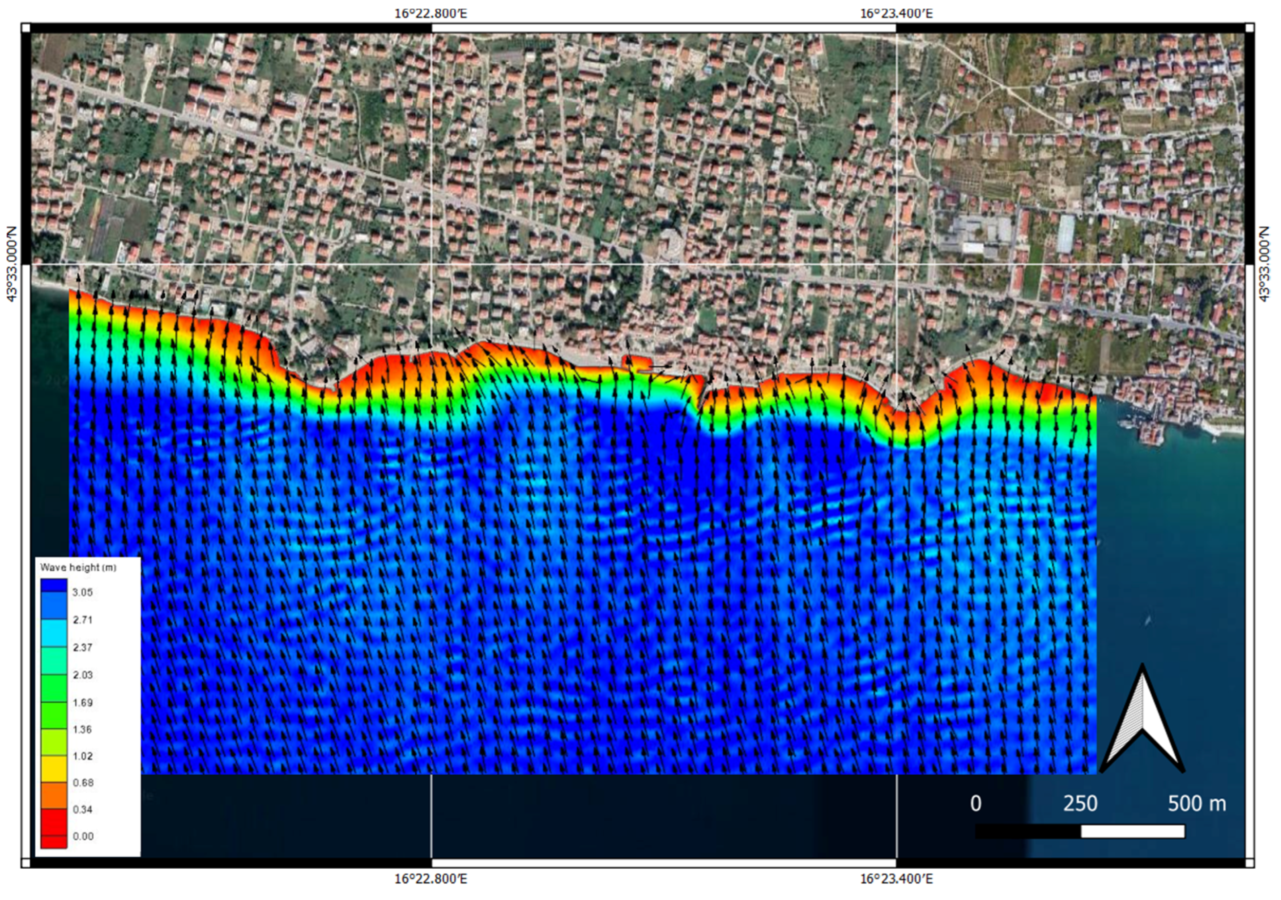
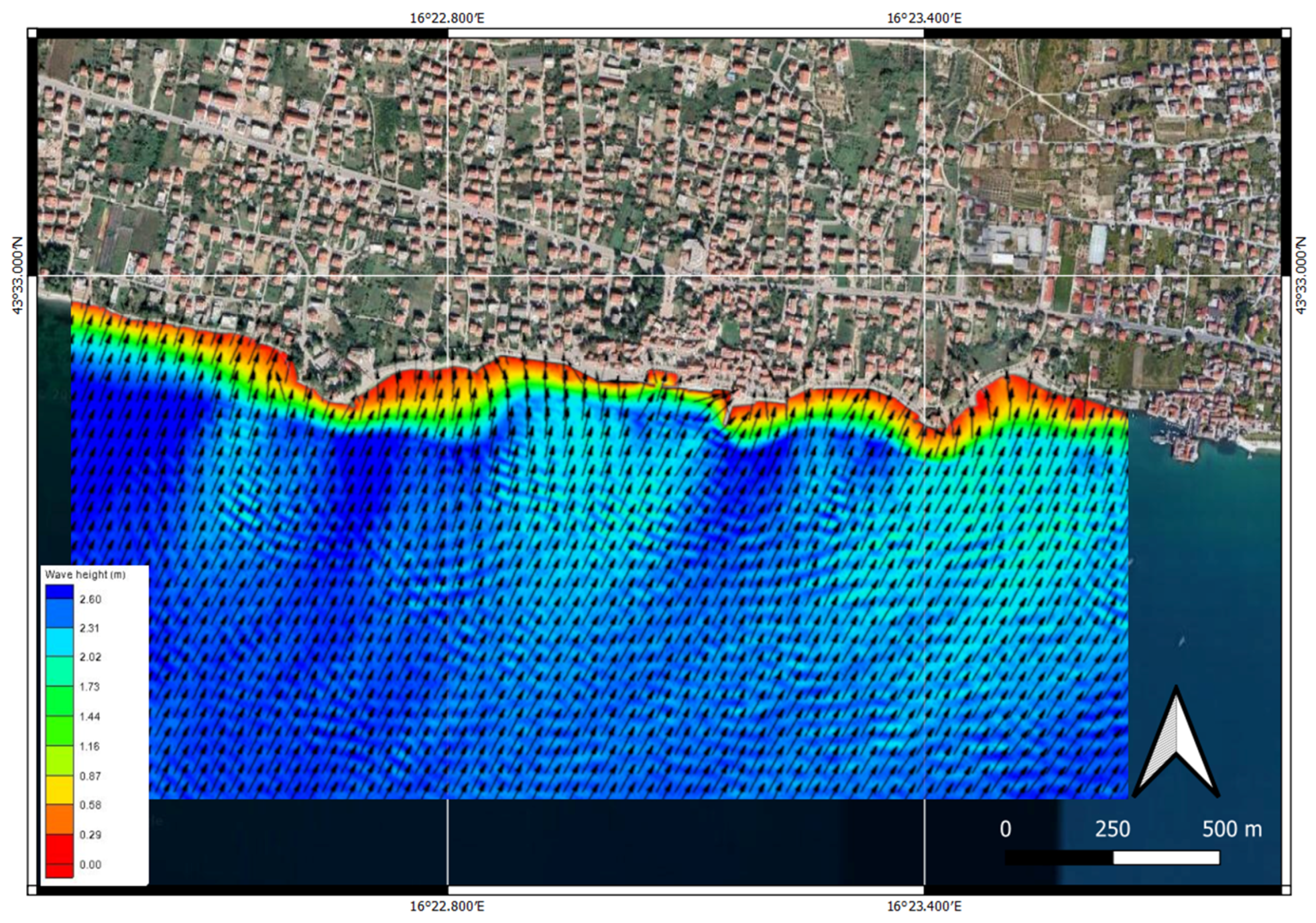
• For relevant incident directions, numerical simulation of the wave transform has been performed by incorporating shoreline reflection coefficients determined on site;
• The study area has been divided into ten zones fundamentally different with regard to reflection features;
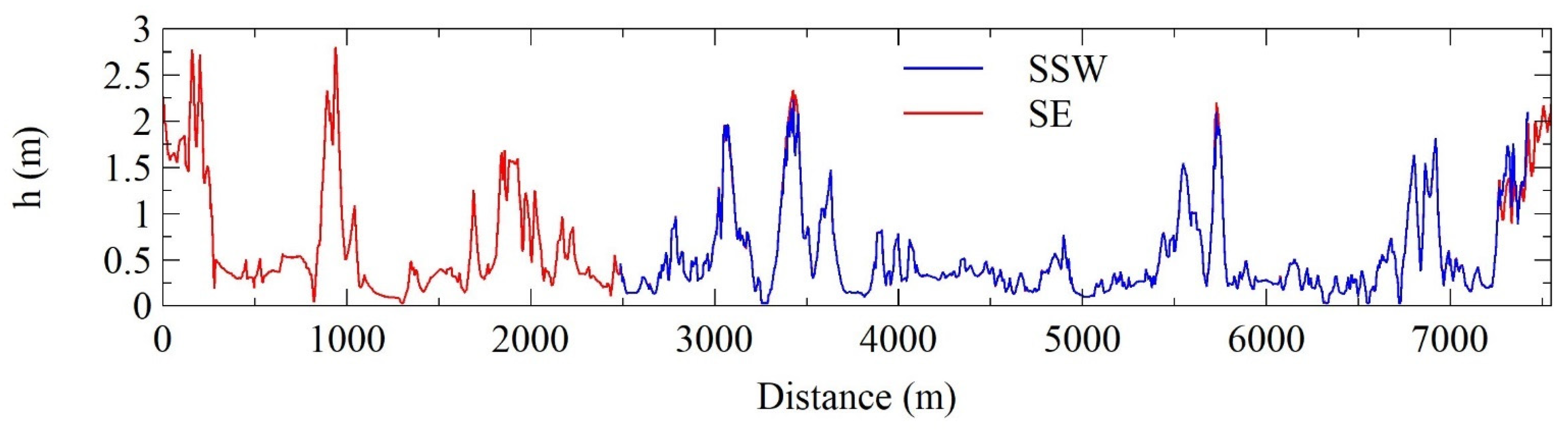
• For each zone wave, parameters have been determined within the zone close to the shoreline (4 m away from the shoreline);
• Final determination of the sea water elevation by incorporating three abovementioned mechanisms is done by:

  $$h_{sea}=h_t+h_{at}+h_{S\left(d=4\mathrm{m}\right)}$$

  (5)

  which offers an easy-to-implement way to assess absolute sea level, where $h_t$ represents the tidally induced component, $h_{at}$ represents the barometric pressure-induced component and $h_{S\left(d=4\mathrm{m}\right)}$ stands for the significant wind-generated height as found 4 m offshore. The value of $h_{sea}$ is expressed relative to HVRS71 datum [33].

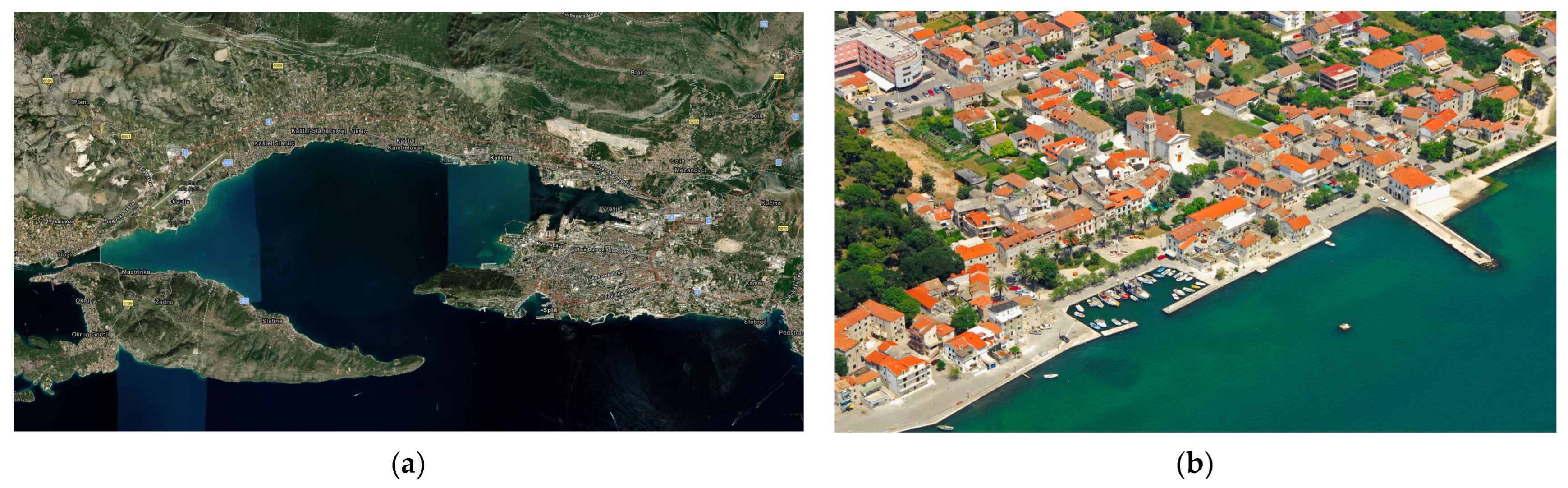
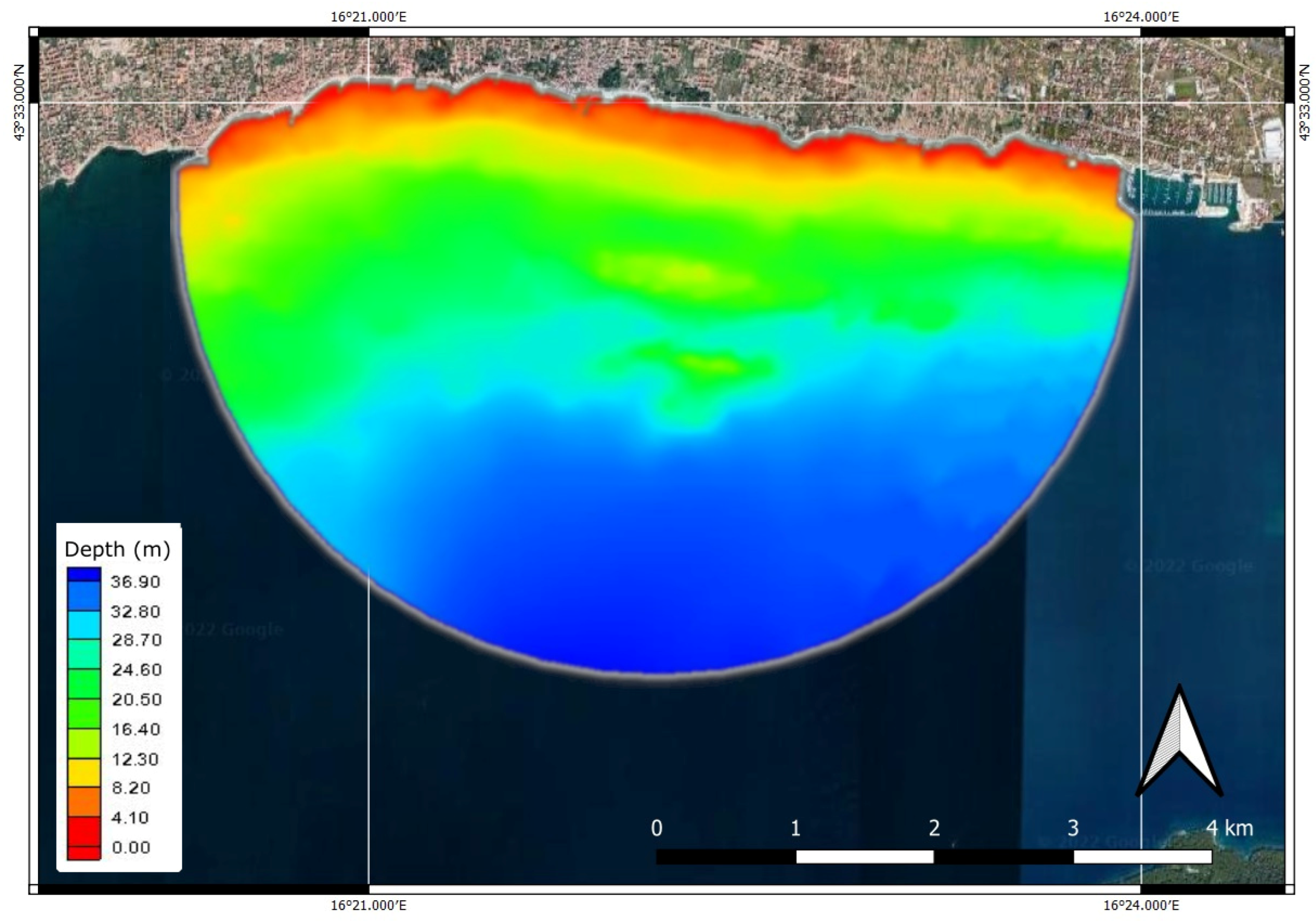
2.2. Site Description

The location of the study area with definition of the tidal gauge and meteorological stations are shown in Figure 3. The meteorological station Split with geographical coordinates φ = 43°31′ N, λ = 16°26′ E is located northwest of the city Split, on the Marjan hill, at the altitude of 122 m a.s.l. The terrain is a slope towards the sea on the SW-W-NW-N side. To the north is the bay of Kaštela and to the east is the city of Split. At a distance of 7 km toward the north is the mountain Kozjak with the highest peak at 779 m a.s.l. The measuring system Fuess [34] is installed at a 5 m high terrace column on the building roof (12 m above ground). The only obstacles found near the meteorological station building are found to the west and northwest side (trees and terrain elevation overgrown with trees more than 10 m tall). The roughness class of the terrain is 2.5 (z₀ = 0.2) [34]. The wind speed and direction data obtained by the classic Feuss measurement consist of an average hourly wind speed with corresponding wind.

The nearest tidal gauge near Kaštela Bay is located within the Institute of Oceanography and Fisheries (IOR) in Split, at the western border of peninsula Marjan. The time series of measured sea surface elevations over a total duration of five years have been obtained from the Marjan tide gauge for the period from 1 January 2010 to 31 December 2014. The sampling frequency of the tide gauge was set to 1 h for the entire time series. The measured water level elevation is referred to as the HVRS71 vertical datum [33]. Due to the maintenance and malfunction of the tide gauge IOR Marjan, the observed time series are characterized by periods without recorded values of the sea level. For the purpose of this work, a continuous time series is required so the longest continuous time series has been found from 25 January 2010 at 12:00 h to 27 June 2011 at 23:00 h with a total of 12,444 h of data.

Barometric pressure data are obtained from two meteorological stations: Split-Airport and Split-Marjan. The meteorological station Split-Airport is located at 21 m a.s.l. and the barometric pressure values are recorded three times a day at 7 am, 2 pm and 9 pm. The meteorological station Split-Marjan is located at 122 m a.s.l. and has an hourly measurement frequency including barometric pressure values. Logs of barometric pressure were obtained from both meteorological stations for the period from 1 January 2010 to 31 December 2014. Due to the location of Kaštela Bay, the meteorological station Split-Airport was considered as relevant, but due to its low measurement frequency (3 times per day), the data from Split-Marjan was used for further analysis. First, the data from Split-Marjan was compared with the data from Split-Airport and a mean difference of 12.67 hPa with a standard deviation of 0.67 hPa was found. All data from Split-Marjan were corrected for the values of 12.67 hPa. The available data from the Split-Marjan station has a continuous record with no missing data for the entire 5-year period. However, since the sea level signal does not have the same continuity as the barometric pressure, the same period of barometric pressure as sea level is included in the further analysis.

Insight into bathymetric features emphasize depth values up to 37 m with a pretty uniform decrease towards the shoreline (Figure 4). A bathymetric survey for the purpose of this paper has been performed in April 2021 with a single beam setup. Shoreline determination of the reflection coefficient has been done at the site by the inspection of both shoreline type and depth in front (Figure 5).

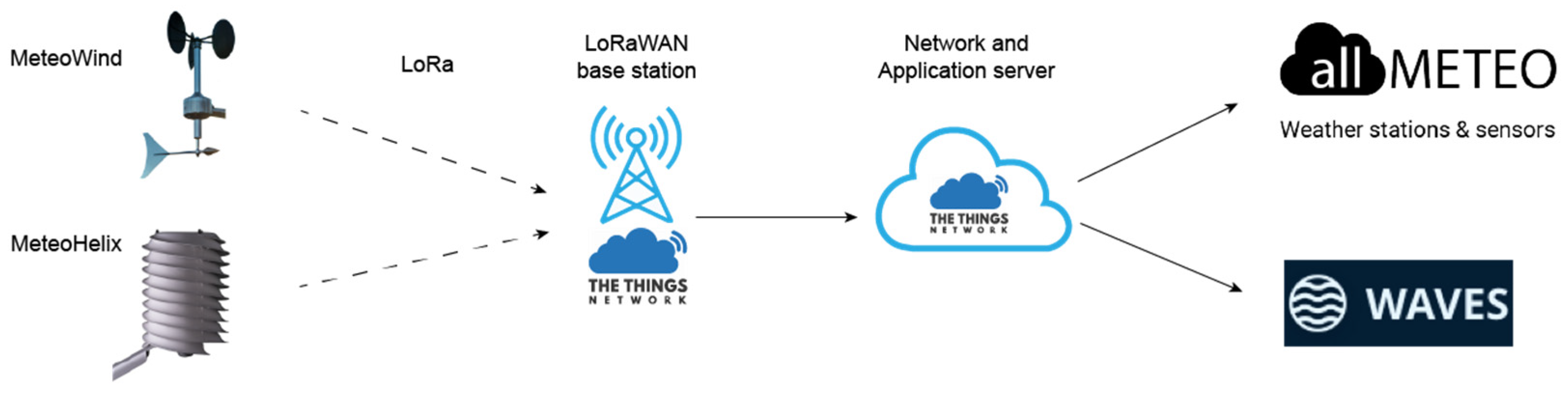
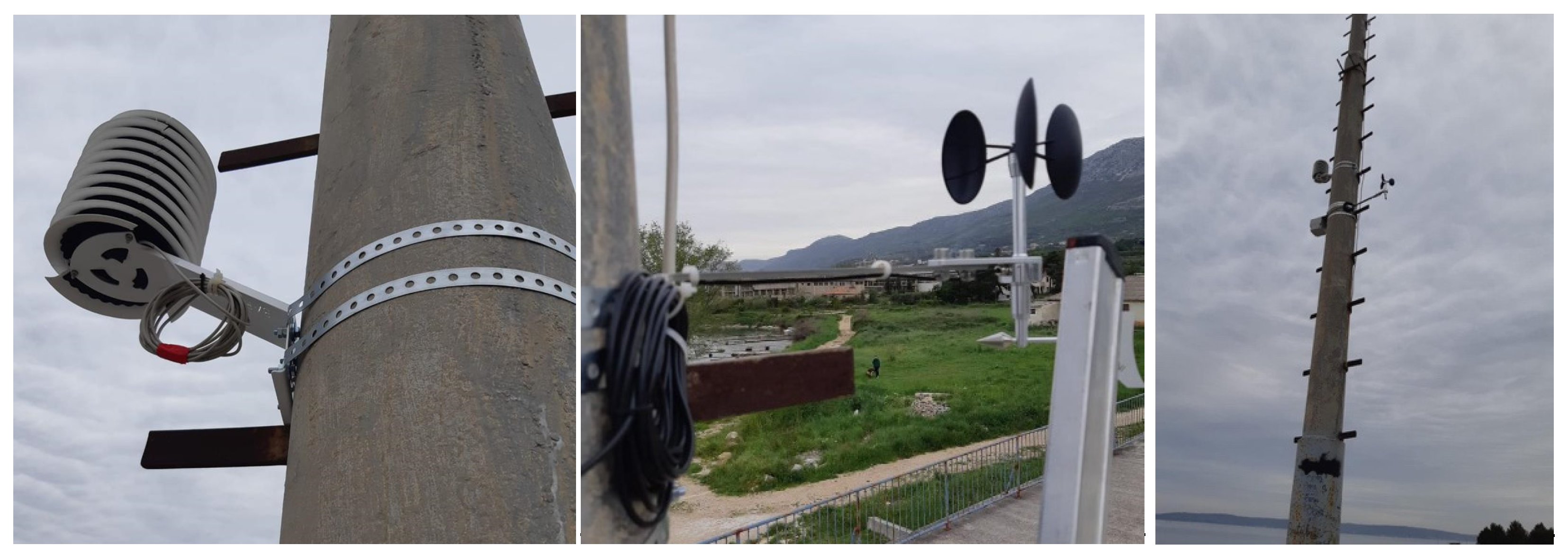
2.3. Data Collection from LoRaWAN-Based Sensor Device

LoRaWAN is one of the most widely used Low Power Wide Area technologies that aims to collect and communicate data from an end sensor device at a large distance, making it perfect for a scenario in which sensor devices collect wind and barometric data and convey them to a centralized system. LoRaWAN employs a typical star-of-star topology where end devices communicate data in a single hop to one or more gateway devices. These messages are further forwarded to the network and application server for further processing, allowing authorized data to be forwarded to other external services (e.g., using MQTT message forwarding). LoRaWAN allows battery-operated devices to periodically transmit sensor data over large distances, while minimizing consumption during inactive periods. LoRaWAN technology finds its application in smart city/smart agriculture environments where there is no need for real-time (every second) transmission from end devices. During the inactive period, end devices simply cut off the consumption, allowing a battery lifetime up to a couple of years without any external power source.

Figure 6 depicts the architecture of the MeteoHelix weather station of Barani design that utilizes LoRaWAN as a radio technology. MeteoHelix [35] is an automatic all-in-one microweather station which is solar powered and can be active for up to 6 months without sun. It measures air temperature to WMO accuracy, air humidity to WMO accuracy with dew and frost point output, barometric pressure and solar irradiation (pyranometer). Another sensor of Barani design was also installed that utilizes LoRaWAN communication—MeteoWind IoT PRO. MeteoWind [36] is used for wind monitoring and employs two sensors: a separate wind vane and anemometer. MeteoWind allows 4+ months of battery life without sun and a maintenance-free service life with long-term measurement stability due to its elliptical cup and metal construction. As depicted in Figure 7, both devices are placed at a 10 m height without any object around within 150 m so that both the wind speed and wind direction are not distorted, while both are located in location of Kaštela Bay. Since both MeteoHelix and MeteoWind IoT PRO employ LoRaWAN communications to convey data over the air to the centralized system, The Things Network as a service provider was used to collect data for further processing. As a LoRaWAN gateway, an indoor Sentrius RG1xx LoRaWAN gateway device placed around 150 m from the sensor devices was employed that forward messages to The Things Network (TTN) cloud infrastructure. Once the message arrives at the gateway, it is forwarded to the TTN Network and Application server. Furthermore, TTN allows message forwarding from TTN infrastructure to our dedicated Waves Seafront Monitoring app using MQTT protocol, which is described more in detail in the following section.

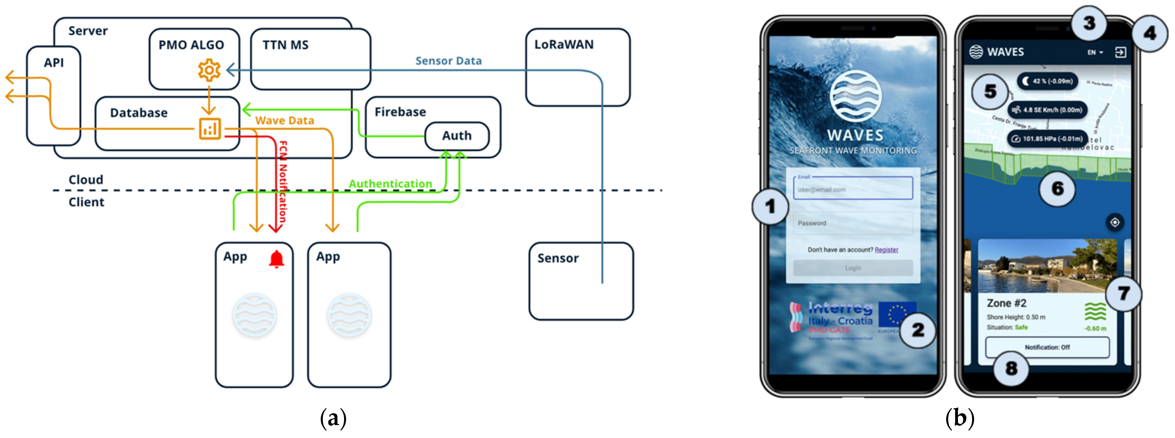
2.4. Waves Seafront Monitoring Architecture—Overview and Functionalities

Waves Seafront Monitoring is a cross-platform mobile application that allows users to access and interactively view the current sea level, discretized by coastal segments with respect to coastal height. As shown in Figure 8a, it comprises a cloud and client side. At the cloud side, the Google Firebase server component executes an evaluation algorithm based on data from the sensor it communicates with, serves as a server for these results and performs user authentication. Sensor data comprising air pressure, wind speed and direction are sent to The Things Network (TTN) cloud via the LoRaWAN communication channel, which is forwarded via MQTT protocol to the TTN microservice. Once the packet with sensor data arrives, the TTN microservice captures and stores the LoRaWAN uplink data into the database and forwards the data through the PMO algorithm to estimate sea level according to the data arriving from LoRaWAN sensors (wind speed and direction, barometric pressure and sea tide level). As can be seen, an alarm notification can be sent to the application if the sea level exceeds a predefined level.

The front-end of the application is comprised of the following elements, as depicted in Figure 8b:

A.

Login interface (Figure 8b)—initial interface for users when opening the application:

• Form—the user enters his login details (e-mail and password) and has the option of registration if he does not have an account by clicking on the appropriate link (Figure 8b, number 1),
• Prominent logo—the project was realized within the Interreg PMO GATE collaboration (Figure 8b, number 2).

B.

Registration Interface—the registration interface is analogous to the login interface, only it allows the user to create an account to access the application by entering login information. To simplify logging into the system, there is no special validation of user accounts, such as email confirmation.

C.

Map interface (Figure 8b) —the central part of the application, which contains the following basic functionalities:

• At the top is a drop-down menu where the user has a choice between three languages: Croatian, English and Italian. By clicking on an option, the interface text adjusts the interface language (Figure 8b, number 3).
• Log out button from the application (Figure 8b, number 4).
• Values read from the sensor are updated over time depending on how often the data from the TTN arrives. From top to bottom, sea level is the sum of altitudes caused by sea tide, wind speed and direction and barometric pressure (Figure 8b, number 5). The total amount is calculated based on the algorithm submitted by the Client.
• Google maps with plotted polygons that correspond to discretized segments of the coast according to their heights (Figure 8b, number 6). The color of the zone corresponds to the early warning status: green—safe, i.e., the sea level is below the coast level; yellow—warning, i.e., the sea can exceed 20 cm above the height of the shore; orange—dangerous, i.e., the sea can rise up to 50 cm above the height of the shore; red—flooded, i.e., the sea exceeds 50 cm above the height of the coast. By clicking on an individual zone, the cards will position themselves next to the corresponding zone and the map will be centered on the selected zone. Based on the coastal height data, the monitoring area is divided into 10 zones.
• Zone maps showing the names and photos of coastal zones. Here, the user can see exactly the height of this segment of the coast, the estimated sea level in relation to the zone and, consequently, the situation in that zone, which is coded in colors analogous to the zones on the map (Figure 8b, number 7). Each zone information contains the sea level with respect to the coastal height, where the number with the minus sign shows how much the sea level is below the coastal height. Once the number becomes positive, the zones change color since this result corresponds with estimated flood. By moving the tabs left or right, the user can focus on a specific zone, and the map will center on that zone.
• Notification button (Figure 8b, number 8). By clicking on this button individually for each zone, the user can indicate whether he wants to receive notifications when the situation in a particular zone changes.

3. Results

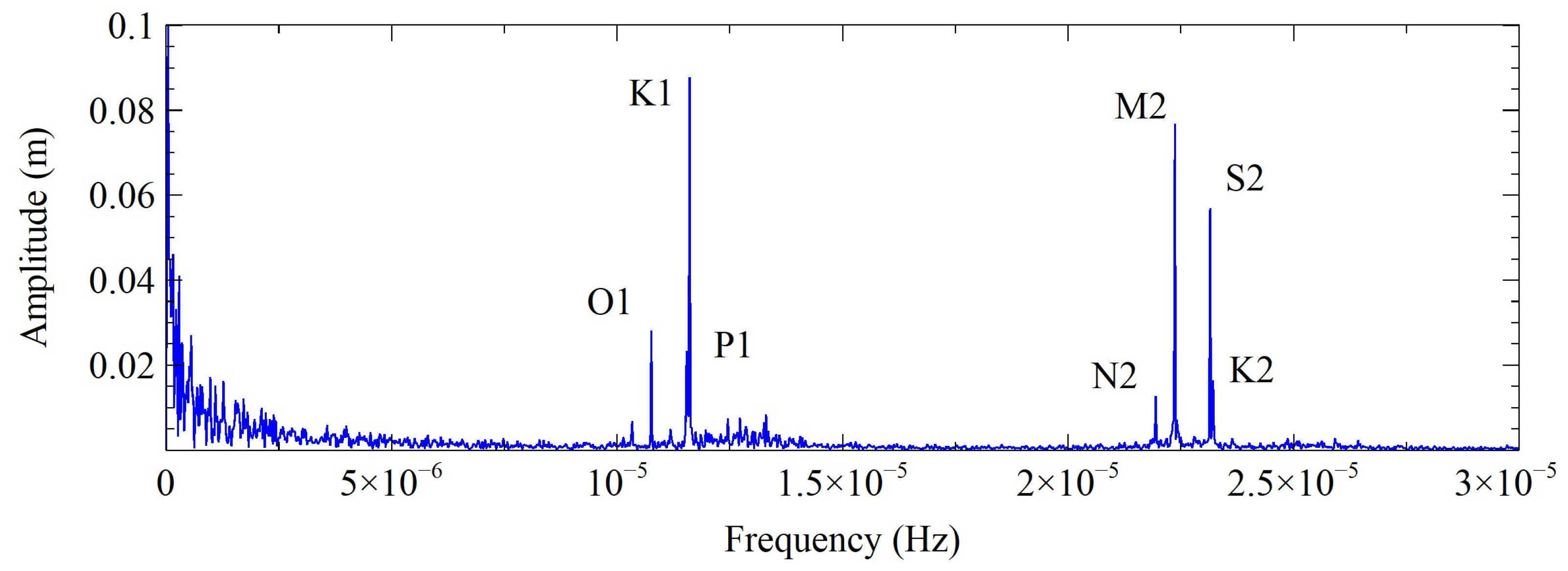
3.1. Sea Level Determination Based on the Tidal Fluctuations

To enable the assessment of tidal-induced sea level oscillations, a total of 12,444 h of observed time series data was used to perform DFT and obtain an amplitude spectrum (Figure 9). Due to the nature of the observed signal, inspection of the amplitude spectrum offers the presence of the trend, visible within the bins corresponding to the lowest frequencies. In total, seven tidal harmonics has been identified as dominant, thus ensuring the tidal-induced sea level oscillation characterization.

While tidal amplitudes and periods were determined directly from the spectrum shown in Figure 9, phases were determined from the complex component of each of the seven tidal harmonics. All characteristic values for the relevant tidal constituents are shown in

Table 1. Tidal constituents with corresponding values of amplitude, period and phase.

Constituent	Amplitude (m)	Period (h)	Phase (°)
O1	0.02821644	25.81743	−160.6065
K1	0.02339150	24.06963	105.3624
P1	0.08773618	23.93077	153.1416
N2	0.01279412	12.65921	65.3833
M2	0.07688095	12.41916	−31.55806
S2	0.05696792	12.00000	−126.8397
K2	0.01636003	11.96538	116.0807

. The quality of the determined harmonic values were checked by the application of the correlation coefficient when applied to both the simulated and observed time series.

Both the observed and simulated sea level signals, one for each 1000 h of the available time series, are compared by using Pearson correlation coefficient and root mean square error. When simulating the sea level by using Equation (2), the simulated signal discovers the absence of the trend within, which is incorporated in the next step as a response to long-term barometric pressure changes. The residual was determined as a difference between the observed and simulated signals. Both signals are shown relative to the HVRS71 vertical datum, as explained in the Methodology section. The same procedure was repeated for each 1000 h data of the total 12,444 h data representing the total sample. Both Pearson correlation coefficient and root mean square error values are shown in

Table 2. Pearson coefficient and root mean square values obtained between the measured and simulated sea water elevation by Equation (2).

Data Sets (h)	0–1000	1000–2000	2000–3000	3000–4000	4000–5000	5000–6000	6000–7000	7000–8000	8000–9000	10,000–11,000	11,000–12,444	0–12,444
RMSE	0.198	0.141	0.083	0.082	0.075	0.071	0.147	0.241	0.091	0.159	0.095	0.136
Pear. Corr. Coef.	0.551	0.597	0.749	0.782	0.923	0.802	0.664	0.639	0.752	0.834	0.791	0.578

.

For the entire observed and simulated set of 12,444 h data, the root mean square value equals to 0.136 [m], while Pearson’s correlation coefficient equals 0.578 [-]. The high value of RMSE and low value of the correlation coefficient indicate the sea level fluctuations are not only subjected to tidal variations, but also to other factors.

3.2. Sea Level Determination Based on the Tidal Fluctuations and Barometric Pressure Changes

Figure 10 shows the effect of barometric pressure on the simulated signal with seven frequencies. The simulated sea level signal has a similar trend to the observed sea level signal with a residual remaining between the simulated and observed signal. When the sea level signal is simulated using the tidal components and the inverted barometric effect, the RMSE decreases to 0.1057 [m] and the Pearson correlation coefficient increases to 0.777 [-], further highlighting the effect of barometric pressure and its contribution to the observed sea level definition at the location of interest (

Table 3. Pearson coefficient and root mean square values obtained between the measured and simulated sea water elevation by Equation (4).

Data Sets (h)	0–1000	1000–2000	2000–3000	3000–4000	4000–5000	5000–6000	6000–7000	7000–8000	8000–9000	10,000–11,000	11,000–12,444	0–12,444
RMSE	0.144	0.103	0.061	0.062	0.083	0.061	0.113	0.189	0.091	0.126	0.076	0.106
Pear. Corr. Coef.	0.735	0.776	0.886	0.886	0.936	0.865	0.886	0.794	0.812	0.891	0.872	0.777

). The decrease in the residual values when both the barometric pressure and tidal effects are involved in the procedure for the sea level determination implies the relevance of those two mechanisms in the vertical movement of sea surface elevation.

3.3. Wind-Generated Waves

Following the knowledge from the location of interest, two relevant wave incident directions have been identified, SE and SSW. The reason for the selection of those two incident directions relies on three facts: (i) longest possible fetch lengths compared to other incident directions, (ii) longest wind duration and wind velocities and (iii) relative position of the shoreline almost perpendicular to the incident directions.

Table 4. Deepwater wave parameters—incident direction SE.

V (ms−1)	t (h)	Fmin (km)	tmin (h)	FEFF (km)	FMJ (km)	HS (m)	TS (s)	L0 (m)
1.5	13	43.36	8.65	24.8	24.8			0
3.3	13	71.25	6.02	24.8	24.8			0
5.4	13	97.17	4.8	24.8	24.8	0.5	2.6	10.55
7.9	13	123.48	4.03	24.8	24.8	0.85	3.15	15.49
10.7	17	215.89	3.5	24.8	24.8	1.21	3.65	20.8
13.8	15	213.49	3.12	24.8	24.8	1.7	4	24.98
17.1	11	159.77	2.82	24.8	24.8	2.19	4.35	29.54
20.7	4	45.07	2.59	24.8	24.8	2.78	4.76	35.38

offers the highest significant wave height equal to 2.78 m with a corresponding period of 4.76 s. For the SSW incident direction,

Table 5. Deepwater wave parameters—incident direction SSW.

V (ms−1)	t (h)	Fmin (km)	tmin (h)	FEFF (km)	FMJ (km)	HS (m)	TS (s)	L0 (m)
1.5	5	11.71	6.68	17.4	11.71			0
3.3	5	19.24	4.65	17.4	17.4			0
5.4	5	26.24	3.7	17.4	17.4	0.5	2.5	9.76
7.9	5	33.35	3.11	17.4	17.4	0.77	2.95	13.59
10.7	5	40.37	2.7	17.4	17.4	1.05	3.15	15.49
13.8	5	34.91	2.41	17.4	17.4	1.41	3.6	20.23
17.1	5	26.94	2.18	17.4	17.4	1.92	3.98	24.73
20.7	5	6.75	2	17.4	6.95	2.35	4.15	26.89

shows the highest wave parameters equal to 2.35 m and 4.15 s.

The procedure for wave height determination at the distance of 4 m offshore starts with known wind velocity and duration. For the selected incident wave direction and fetch length, deep wave parameters have been selected from Table 4 and Table 5. For the purpose of wave height determination in front of the shoreline, the JONSWAP spectrum is used to incorporate a real wave into the wave transform model. Spectrum parameters have been set up as shown in

Table 6. Deepwater wave parameters—JONSWAP spectrum parameters.

Incident Direction	Hs (m)	T (s)	γ	nn
SE (165°)	3.05	6.40	3.30	4.00
SSW (202.5°)	2.60	5.90	3.30	4.00

, where the obtained deep water wave values correspond to a 100-year return period.

Wave height spatial distribution and direction for the SE incident wave direction is presented in Figure 11. Insight into the inner zone of interest discovers the presence of refraction as a main wave transform mechanism. The insight into significant wave height changes at 4 m offshore is shown in Figure 12 and Figure 13. The same has been shown for the SSW incident direction in Figure 12 and Figure 13. By comparing modeled wave heights, it is obvious the SE incident direction results in more significant wave height values.

3.4. Real-Time Prediction of Sea Water Elevation and Warning

The monitoring system has been installed and put into operation at the Kaštela Bay test site to provide real-time measurement of wind speed, wind direction and barometric pressure. The observed data is used for the real-time prediction of sea level based on the developed algorithm for the estimation of sea level heights and information obtained from the monitoring system, which has been integrated into the algorithm. The real-time prediction of sea level values is obtained based on tidal fluctuations, barometric pressure values and wind characteristics.

Resulting sea level values are compared with coastline elevation in order to identify the potential danger of flooding and issue on-time warnings. Figure 14 shows wind characteristics and barometric pressure as observed during a period of 7 days during February 2022. The data containing barometric pressure along with wind direction and speed were collected into a database for the application. The data were used as an input for an algorithm to estimate sea level height.

Figure 15 shows sea water elevation as a consequence of each of the components (tidal effect, barometric pressure and wind-generated waves) as well as absolute sea water elevation as a superposition of the abovementioned components for the period from 15 December 2021–7 February 2022. The results are given for one randomly selected zone along the study area to demonstrate the capacity of the proposed procedure to assess the sea water elevation. The estimated water surface elevation is referred to the HVRS71 vertical reference datum determined on the basis of mean sea level, as stated in the Methodology section.

If the resulting sea level value estimated from the algorithm exceeds the coastline elevation, the warning is immediately issued by the mobile application to alert the endangered population. Flood hazard warnings in the mobile application are primarily focused on citizens’ safety and their classification is based on the particular threat level. Threat levels are based on tests of the instability of a human body in floodwater and different stability thresholds [37]. Following the results of the tests, the first threat level, issuing a yellow alert, is defined for flood water depth on the coastline up to 20 cm, which is mostly threatening for children. The second level of threat corresponds to an orange warning, which is now becoming dangerous for adults and is issued when the water depth is between 20 cm and 50 cm. Finally, an exceedance of flood water depth over 50 cm on the coastline corresponds to the third threat level. In this case, severe injuries can be caused by flood water and the red warning for the population is issued.

4. Discussion

In this paper, a procedure to assess sea water elevation caused by coastal flooding at Kaštela Bay is presented, together with the monitoring system infrastructure scheme and sea water elevation prediction module. In its origin, the procedure relies on the real-time monitoring IoT-based system for sea level-relevant parameter monitoring to capture wind-generated wave heights and barometric pressure-induced sea level changes.

The latter offers the possibility to determine wind-generated wave heights in front of the coast, with an incorporation of shoreline reflection features as assessed by the sea water depth and type of structure found at the site, and long- and short-term changes in the mean sea water level. Tidal-induced sea level changes are forecasted based on the data series observation from the nearest relevant tidal gauge.

After wind speed/direction and barometric pressure sensors are installed at the site to enable real-time monitoring, a LoRaWAN-based IoT monitoring system was employed, along with the dedicated cross-platform mobile application, which was used as an early warning notification system. Therein, registered end users can set early warning notifications based on their zone of interest.

As stated, the origin of the presented approach relies on the capability of the monitoring system to observe the wind speed/direction and barometric pressure at the site. The selection of the location of the monitoring infrastructure is performed at the location of interest to neglect spatial variations in barometric pressure variations and offer reliable input for barometric pressure-induced sea level changes.

Relevant mechanisms acting to assess the sea water elevation are selected based on the phenomena characterizing the study area and fit suitable for the pre-assumed conditions mostly found on site. The effect of barometric pressure changes and their influence on mean sea water elevation refers to the sea in a calm state and static conditions when no significant changes in the barometric pressure field are observed. In case this requirement is not met, such as when the storm is moving, a difference in predicted sea level changes compared to real ones can be obtained.

Our results demonstrate the capability of the proposed methodology to enable a realistic and reliable forecast of the sea water elevation by taking into consideration local conditions: (i) wind information, (ii) barometric pressure, (iii) tidal forcing, (iv) water depth and (v) coastal structure or type information.

When coupled with the shoreline’s absolute height, one is enabled to assess flooding risk or the vulnerability of the coast to sea level-induced flooding. The developed monitoring system, coupled with data collection from LoRaWAN-based sensor device and assessment procedure, presents a unique and robust approach to be used along different coastal areas of the Adriatic Sea.

Apart from this, different coastal structures found along the specific site can easily be taken into consideration by assessing the reflectance features from the structure type and bathymetric features in front of the coastline.

5. Conclusions

This paper presents a procedure to assess the coastal flooding induced by the sea level in the Kaštela study area. In its origin, it consisted of three modes: (i) the LoRaWAN-based sensor device monitoring infrastructure located at the site to capture relevant parameters in real time, (ii) a step-by-step procedure to assess the sea water elevation and (iii) Waves Seafront Monitoring cross-platform mobile application to enable the real-time insight into coastal flooding occurrence. The main conclusions obtained from the study can be summarized as:

• The presented procedure to assess coastal flooding induced by seawater has been shown to be efficient when applied to the Kaštela study area.
• The origin of the assessment for the seawater elevation relies on three basic mechanisms: tidal oscillations, barometric pressure-induced oscillations and wind-generated waves. Despite the potential limitation, no significant deflection from the sea water elevation occurred at the site during the period from 15 December 2021 to 7 February 2022 was observed.
• The presented procedure shows robustness in the potential to incorporate other relevant mechanisms influencing sea water elevation and site-specific features. It can be extended to the relevant mechanisms acting toward the sea level definition and adjusted to the local conditions reflecting the site-specific features. In case of need, additional effects can be added: (i) submerged structures overtopping, (ii) wave run-up, (iii) seiche, (iv) beach or shoreline friction effects, (v) dynamic inverse barometric effects, (vi) coastal flooding induced by the precipitation, especially during the cyclone and its superposition with the sea-induced flooding. The latter not only contributes to enhanced capacity of the coastal flooding awareness at the Kaštela site, but also enables the procedure to be applied at other sites.

References

1. IPCC. Changes in climate extremes and their impacts on the natural physical environment. In Managing the Risks of Extreme Events and Disasters to Advance Climate Change Adaptation; Field, C.B., Barros, V., Stocker, T.F., Dahe, Q., Dokken, D.J., Ebi, K.L., Mastrandrea, M., Mach, K.J., Plattner, G.K., Allen, S.K., et al., Eds.; Cambridge University Press: Cambridge, UK; New York, NY, USA, 2012; pp. 109–230. [Google Scholar]
2. Petroliagkis, T.I.; Voukouvalas, E.; Disperati, J.; Bidlot, J. Joint Probabilities of Storm Surge, Significant Wave Height and River Discharge Components of Coastal Flooding Events. In Utilising Statistical Dependence Methodologies and Techniques, JCR Technical Reports; Publications Office of the European Union: Luxembourg, 2016. [Google Scholar]
3. Tsoukala, V.K.; Chondros, M.; Kapelonis, Z.G.; Martzikos, N.; Lykou, A.; Belibassakis, K.; Makropoulos, C. An integrated wave modelling framework for extreme and rare events for climate change in coastal areas—The case of Rethymno, Crete. Oceanologia 2016, 58, 71–89. [Google Scholar] [CrossRef] [Green Version]
4. Gallien, T.; Sanders, B.; Flick, R. Urban coastal flood prediction: Integrating wave overtopping, flood defenses and drainage. Coast. Eng. 2014, 91, 18–28. [Google Scholar] [CrossRef]
5. Barnard, P.L.; Van Ormondt, M.; Erikson, L.H.; Eshleman, J.; Hapke, C.; Ruggiero, P.; Adams, P.; Foxgrover, A.C. Development of the Coastal Storm Modeling System (CoSMoS) for predicting the impact of storms on high-energy, active-margin coasts. Nat. Hazards 2014, 74, 1095–1125. [Google Scholar] [CrossRef]
6. Mendoza, E.T.; Jimenez, J.A. Regional vulnerability analysis of Catalan beaches to storms. In Proceedings of the Institution of Civil Engineers—Maritime Engineering; Thomas Telford Ltd.: London, UK, 2009; Volume 162, pp. 127–135. [Google Scholar]
7. De Kleermaeker, S.; Verlaan, M.; Kroos, J.; Zijl, F. A new coastal flood forecasting system for the Netherlands. In Proceedings of the Hydro12 Conference Proceedings: Taking Care of the Sea, Rotterdam, The Netherlands, 13–15 November 2012; Dorst, L., van Dijk, T., van Ree, R., Boers, J., Brink, W., Kinneging, N., van Lancker, V., de Wulf, A., Nolte, H., Eds.; Hydrographic Society Benelux: Heeg, The Netherlands, 2012. [Google Scholar] [CrossRef] [Green Version]
8. Doong, D.-J.; Chuang, L.Z.H.; Wu, L.-C.; Fan, Y.-M.; Kao, C.C.; Wang, J.-H. Development of an operational coastal flooding early warning system. Nat. Hazards Earth Syst. Sci. 2012, 12, 379–390. [Google Scholar] [CrossRef] [Green Version]
9. Bogaard, T.; De Kleermaeker, S.; Jaeger, W.S.; Van Dongeren, A. Development of Generic Tools for Coastal Early Warning and Decision Support. In Proceedings of the E3S Web of Conferences—3rd European Conference on Flood Risk Management (FLOODrisk 2016), Lyon, France, 17–21 October 2016; EDP Sciences: Paris, France, 2016; Volume 7, p. 18017. [Google Scholar] [CrossRef] [Green Version]
10. Dreier, N.; Fröhle, P. Operational wave forecast in the German Bight as part of a sensor and risk based early warning system. J. Coast. Res. 2018, 85, 1161–1165. [Google Scholar] [CrossRef] [Green Version]
11. Merrifield, M.A.; Johnson, M.; Guza, R.T.; Fiedler, J.W.; Young, A.P.; Henderson, C.S.; Lange, A.M.Z.; O’Reilly, W.C.; Ludka, B.C.; Okihiro, M.; et al. An early warning system for wave-driven coastal flooding at Imperial Beach, CA. Nat. Hazards 2021, 108, 2591–2612. [Google Scholar] [CrossRef]
12. Memos, C.; Makris, C.; Metallinos, A.; Karambas, T.; Zissis, D.; Chondros, M.; Spiliopoulos, G.; Emmanouilidou, M.; Papadimitriou, A.; Baltikas, V.; et al. Accu-Waves: A decision support tool for navigation safety in ports. In Proceedings of the 1st In-ternational Conference Design and Management of Port, Coastal and Offshore Works (DMPCO), Athens, Greece, 8–11 May 2019. [Google Scholar]
13. Makris, C.; Androulidakis, Y.; Karambas, T.; Papadimitriou, A.; Metallinos, A.; Kontos, Y.; Baltikas, V.; Chondros, M.; Krestenitis, Y.; Tsoukala, V.; et al. Integrated modelling of sea-state forecasts for safe navigation and operational management in ports: Application in the Mediterranean Sea. Appl. Math. Model. 2020, 89, 1206–1234. [Google Scholar] [CrossRef]
14. Spiliopoulos, G.; Bereta, K.; Zissis, D.; Memos, C.; Makris, C.; Metallinos, A.; Ka-rambas, T.; Chondros, M.; Emmanouilidou, M.; Papadimitriou, A.; et al. A Big Data framework for Modelling and Simulating high-resolution hydrodynamic models in sea harbours. In Proceedings of the Global Oceans 2020: Singapore–USA Gulf Coast, Biloxi, MS, USA, 5–30 October 2020; IEEE: New York, NY, USA, 2020; pp. 1–5. [Google Scholar]
15. Mosavi, A.; Ozturk, P.; Chau, K.-W. Flood Prediction Using Machine Learning Models: Literature Review. Water 2018, 10, 1536. [Google Scholar] [CrossRef]
16. Chondros, M.; Metallinos, A.; Papadimitriou, A.; Memos, C.; Vasiliki, T. A Coastal Flood Early-Warning System Based on Offshore Sea State Forecasts and Artificial Neural Networks. J. Mar. Sci. Eng. 2021, 9, 1272. [Google Scholar] [CrossRef]
17. Atzori, L.; Iera, A.; Morabito, G. The Internet of Things: A survey. Comput. Netw. 2010, 54, 2787–2805. [Google Scholar] [CrossRef]
18. Nižetić, S.; Šolić, P.; López-de-Ipiña González-de-Artaza, D.; Patrono, L. Internet of Things (IoT): Opportunities, issues and challenges towards a smart and sustainable future. J. Clean. Prod. 2020, 274, 122877. [Google Scholar] [CrossRef] [PubMed]
19. Reda, H.T.; Daely, P.T.; Kharel, J.; Shin, S.Y. On the application of IoT: Meteorological information display system based on LoRa wireless communication. IETE Tech. Rev. 2018, 35, 256–265. [Google Scholar] [CrossRef]
20. LÓpez-Vargas, A.; Fuentes, M.; Vivar, M. On the application of IoT for real-time monitoring of small stand-alone PV systems: Results from a new smart datalogger. In Proceedings of the 2018 IEEE 7th World Conference on Photovoltaic Energy Conversion (WCPEC) (A Joint Conference of 45th IEEE PVSC, 28th PVSEC & 34th EU PVSEC), Waikoloa, HI, USA, 10–15 June 2018; pp. 605–607. [Google Scholar] [CrossRef]
21. Idier, D.; Aurouet, A.; Bachoc, F.; Baills, A.; Betancourt, J.; Gamboa, F.; Klein, T.; López-Lopera, A.F.; Pedreros, R.; Rohmer, J.; et al. A User-Oriented Local Coastal Flooding Early Warning System Using Metamodelling Techniques. J. Mar. Sci. Eng. 2021, 9, 1191. [Google Scholar] [CrossRef]
22. Janeković, I.; Kuzmić, M. Numerical simulation of the Adriatic Sea principal tidal constituents. Ann. Geophys. 2005, 23, 3207–3218. [Google Scholar] [CrossRef] [Green Version]
23. Press, W.; Teukolsky, S.; Vetterline, W.T.; Flannery, B.P. Numerical Recipes: The Art of Scientific Computing; Cambridge University Press: Cambridge, UK, 2007. [Google Scholar]
24. Cooley, J.W.; Tukey, J.W. An algorithm for the machine calculation of complex Fourier series. Math. Comput. 1965, 19, 297–301. [Google Scholar] [CrossRef]
25. Ponte, R.M. Variability in a homogeneous global ocean forced by barometric pressure. Dyn. Atmos. Ocean. 1993, 18, 209–234. [Google Scholar] [CrossRef]
26. The Effect of Fetch Width on Wave Generation, US Corps of Engineers, Technical Memorandum No. 70. 1954. Available online: https://usace.contentdm.oclc.org/digital/api/collection/p266001coll1/id/7549/download (accessed on 27 July 2021).
27. Goda, J. Revisiting Wilson’s Formulas for Simplified Wind-Wave Prediction. J. Waterw. Port Coast.Ocean Eng. 2003, 129, 2003. [Google Scholar] [CrossRef]
28. World Meteorological Organization, Guide to Wave Analysis and Forecasting, Geneve, Switzerland. 2018. Available online: https://library.wmo.int/doc_num.php?explnum_id=10979 (accessed on 31 July 2021).
29. SMS 13.2 Tutorial CGWAVE Analysis, Aquaveo, v13.2. USA. 2012. Available online: https://www.aquaveo.com/software/sms-learning-tutorials (accessed on 17 August 2021).
30. Demirbilek, Z.; Panchang, V. CGWAVE: A Coastal Surface Water Wave Model of the Mild Slope Equation; Technical Report CHL-98-26; US Army Corps of Engineering: Washington, DC, USA, 1998. [Google Scholar]
31. Panchang, G.V.; Wei, G.; Pearce, R.B.; Briggs, J.M. Numerical Simulation of Irregular Wave Propagation over Shoal. J. Waterw. Port Coast. Ocean. Eng. 1990, 116, 324–340. [Google Scholar] [CrossRef]
32. Zhao, L.; Panchang, V.; Chen, W.; Demirbilek, Z.; Chhabbra, N. Simulation of wave breaking effects in two-dimensional elliptic harbor wave models. Coast. Eng. 2001, 42, 359–373. [Google Scholar] [CrossRef]
33. Brockmann, E.; Harsson, B.-G.; Ihde, J. Geodetic Reference System of the Republic of Croatia—Consultants Final Report on Horizontal and Vertical Datum Definition, Map Projection and Basic Networks for the state geodetic administration of the Republic of Croatia. 2001; 1–35. [Google Scholar]
34. Croatian Meteorological and Hydrological Service. Report of Measured Wind Properties on Gauging Station Marjan. 2011. (In Croatian)
35. BARANI DESIGN Technologies, “MeteoHelix® IoT Pro”. Available online: https://static1.squarespace.com/static/597dc443914e6bed5fd30dcc/t/5f5f9ce8e52f900a7f1982af/1600101615389/MeteoHelix+IoT+Pro+DataSheet.pdf (accessed on 30 March 2022).
36. BARANI DESIGN Technologies, “MeteoWind® IoT Pro”. Available online: https://static1.squarespace.com/static/597dc443914e6bed5fd30dcc/t/5f1813e0fd8f9a4a19feb781/1595413481804/MeteoWind+IoT+Pro+DataSheet.pdf (accessed on 30 March 2022).
37. Xia, J.; Falconer, R.A.; Xiao, X.; Wang, Y. New criterion for stability of a human body in floodwaters. J. Hydraul. Res. 2014, 52, 93–104. [Google Scholar] [CrossRef]
Figure 1. (a) Location of the city of Kaštela in Kaštela Bay; (b) A view of an old historical core, Kaštel Kambelovac.
Applsci 12 12776 g001
Figure 2. Coastal flooding events in the city of Kaštela.
Applsci 12 12776 g002
Figure 3. Location of the study area with the definition of the tidal gauge and meteorological stations (IOR—Institute of Oceanography and Fisheries).
Applsci 12 12776 g003
Figure 4. Bathymetric features at the location of interest.
Applsci 12 12776 g004
Figure 5. Shoreline reflection coefficient along the coastline.
Applsci 12 12776 g005
Figure 6. Architecture of LoRaWAN-enabled MeteoHelix and MeteoWind devices from Barani Design.
Applsci 12 12776 g006
Figure 7. Installation of MeteoHelix and MeteoWind IoT Pro devices.
Applsci 12 12776 g007
Figure 8. (a) High-level overview of the implementation of the solution, (b) Front-end interface of the mobile application.
Applsci 12 12776 g008
Figure 9. Amplitude Spectral Density for observed sea level reduced for the mean value.
Applsci 12 12776 g009
Figure 10. (a) Observed and simulated sea level by Equation (4) for the first 1000 h of observed sea level signals, (b) Observed barometric pressure, (c) Residual between simulated and observed sea level signals.
Applsci 12 12776 g010
Figure 11. Wave heights and directions for the SE incident direction—local study area.
Applsci 12 12776 g011
Figure 12. Wave heights and directions for the SSW incident direction—local study area.
Applsci 12 12776 g012
Figure 13. Modeled wave heights along the control line—incident directions: SE and SSW.
Applsci 12 12776 g013
Figure 14. LoRaWAN-obtained observed time series: (a) wind speed, (b) wind direction and (c) barometric pressure.
Applsci 12 12776 g014
Figure 15. Calculated sea level height during the period from 15 December 2021–7 February 2022 caused by: (a) tidal effect, (b) barometric pressure-induced sea level changes, (c) wind-generated wave height and (d) absolute sea level height.
Applsci 12 12776 g015