Electric Field Induced Drift of Bacterial Protein Toxins of Foodborne Pathogens Staphylococcus aureus and Escherichia coli from Water

Abstract

Bacterial protein toxins secreted by foodborne pathogens, such as Staphylococcus aureus and Shiga toxin-producing Escherichia coli (STEC) strains, may cause severe toxicosis in humans if present in foods or water and constitute an important public health problem. These toxins are large biomolecules with negative and positive ions due to the ionizable groups in the residual amino acids. An innovative theoretical model of purifying aqueous flowing solutions from ionic toxins is proposed in this study. The principle of the model is based on the drift of the ionic toxins, under the application of the external electric field, towards the walls of the duct, leaving the largest part of the duct with reduced levels of toxin. Parameters, such as toxin concentration, potential and electric field intensity distributions, and surface charge densities, are studied analytically for various duct widths and various external electric fields. The proposed model succeeded to reduce toxin levels by more than 99%, for duct widths less than 1cm, making it suitable for small-scale water purification.

1. Introduction

Bacterial toxins produced from foodborne pathogenic microorganisms are proteins that act as virulence factors and may cause a foodborne disease if ingested in food or water. It is estimated that in Europe, bacterial toxins account for approximately 10% of all reported foodborne diseases [1]. Two of the most established foodborne pathogens are Staphylococcus aureus and Escherichia coli. S. aureus is a Gram-positive bacterium that colonizes the skin and nasal cavities of about 50% of healthy individuals, but is also common in livestock, foods, and natural water environments [2,3,4]. S. aureus can survive under unfavorable conditions (e.g., low water activity) at a wide range of temperatures from 7 to 40 °C. Hence, these bacteria are widely dispersed and persist in the environment [5]. S. aureus produces a wide variety of toxic proteins which are secreted outside the bacterial cells (exoproteins) and help the bacteria to colonize and induce disease in mammalian hosts [4]. The main staphylococcal exoproteins are: hemolysins (alpha, beta, gamma, and delta), staphylococcal enterotoxins, Toxic Shock Syndrome Toxin-1 (TSST-1), exfoliative toxins (ETA and ETB), and leukocidin. TSST-1 and the staphylococcal enterotoxins are also called Pyrogenic Toxin Super Antigens (PTSAgs) and are non-glycosylated low molecular weight polypeptides [6,7] which are resistant to various processes, such as proteolysis, denaturation by boiling and chemical inactivation, drying, and freezing [8]. Therefore, these toxins may remain active in food, water, or the passage through the digestive system, even after the death of S. aureus by thermal or other treatments. The most common staphylococcal enterotoxins are SEA and SEB, the first being most frequently involved in staphylococcal food poisoning. The other important category of staphylococcal protein toxins are the hemolysins which cause the lysis of red blood cells. The most common hemolysin is Hla (α hemolysin) which has a beta-barrel structure that attaches to the cell membrane and disrupts it by forming pores, causing osmotic changes that result in apoptotic cell-death [2,9].

Apart from the well-known protein toxins of Staphylococcus, many other bacterial toxins have been characterized in recent years such as the toxins produced by the gram-negative bacterium Escherichia coli O157:H7, which is one of the most pathogenic serotypes of the common foodborne pathogen E. coli. These virulent strains of E. coli are called Shiga toxin producing E. coli (STEC) because they secrete a potent exotoxin called Shiga toxin (Stx) that destroys host cells by inhibiting protein synthesis [10,11]. Shiga toxins are found in two similar forms, Stx1 and Stx2, with Stx2 being far more virulent in vivo in humans than Stx1, resulting in cases of fatal disease such as the hemolytic uremic syndrome [12,13,14]. Stx protein, like other bacterial toxins, has a structure consisting of two subunits, an A-subunit that is surrounded by a ring of five identical B- subunits (AB₅) [15].

Electric field induced drift method has been successfully applied for water desalination and purification from heavy metals [16,17,18]. A similar analysis in nanochannels [19,20,21] with the use of molecular analysis simulation showed that this method can successfully drift ions. A prerequisite of this method is that the molecules to be removed should have electric charge, so that in the presence of an electric field they are forced to migrate towards a specific pole. According to the method, the aqueous solution containing the ions flow inside the duct of the applied electric field. Therefore, ions are forced to migrate towards a specific pole of the electric field, and this drift results in decreasing their concentration in the largest part of the duct.

In this study, an attempt was made to develop a theoretical model through the application of electric field drift in order to reduce the bacterial toxin load from aquatic environments. Four bacterial protein toxins were selected: three toxins of S. aureus (alpha-hemolysin, TSST-1, enterotoxin A) and one of E. coli (Shiga toxin Stx2). Furthermore, in order to construct the model, the device used to induce the electric field drift was described and parameters, such as the final spatial distribution of the concentration, electric field intensity, surface charge density, and potential, were calculated for low voltage. Finally, the time per unit width required for the drift movement is calculated using the analytical solutions of Nernst Planck equations in the linear regime for low voltages, as a function of their overflow protons or electrons, the applied electric field intensity, and the width of the duct.

2. Materials and Methods

2.1. Characteristics of Bacterial Toxins

The physical and chemical characteristics of the four toxin proteins studied are presented in

Table 1. Characteristics of examined toxins.

Type of Toxin	Toxin 1 Staphylococcus aureus Alpha-Hemolysin	Toxin 2: Staphylococcus aureus Toxic Shock Syndrome Toxin-1 (TSST-1)	Toxin 3: Staphylococcus aureus Enterotoxin Type A	Toxin 4: E. coli Shiga Toxin 2 (One Subunit A and Five Subunits B)
Reference	GenBank: QTN48712.1	GenBank: KIT87450.1	GenBank: QTN49470.1	Shiga toxin Stx2 subunit A [Escherichia phage Lyz12581Vzw] NCBI Reference Sequence: YP_009907811.1 Shiga toxin Stx2 subunit B [Escherichia phage Lyz12581Vzw] GenBank: QDF15669.1
Number of amino acids	319	234	257	subunit A: 260 subunit B: 89
Isoelectric point (pI)	8.511	8.615	7.938	6.282
Net charge (at pH 7.4) z	+2.318	+2.392	+1.176	−7.644
Molecular formula	C1592H2481N433O500S9	C1196H1885N305O363S4	C1334H2067N353O404S5	C3462H5407N925O1068S43
Average mass (Da)	35,975	26,473	29,674	78,454
Diffusion coefficient D (m2/s)	$8.11\times {10}^{-11}$	$9.06\times {10}^{-11}$	$8.72\times {10}^{-11}$	$6.31\times {10}^{-11}$
Effective Radius r (m)	$2.71\times {10}^{-9}$	$2.43\times {10}^{-9}$	$2.52\times {10}^{-9}$	$3.49\times {10}^{-9}$
Diameter α (m)	$5.42\times {10}^{-9}$	$4.86\times {10}^{-9}$	$5.04\times {10}^{-9}$	$6.98\times {10}^{-9}$
${\lambda }_S$ (m) (effective width of the Helmholtz capacitor)	$2.71\times {10}^{-9}$	$2.43\times {10}^{-9}$	$2.52\times {10}^{-9}$	$3.49\times {10}^{-9}$

. Calculations of the net protein charge (at pH 7.4), protein isoelectric point and average mass were performed with the free bioinformatic tool Prot-pi which has been developed in collaboration with the Center for Biochemistry and Bioanalytics at Zurich University of Applied Sciences (https://www.protpi.ch/Calculator, accessed on 1 October 2022). The diffusion coefficient of the proteins was calculated with the free on-line calculator (https://www.cytivalifesciences.com/en/us/solutions/protein-research/products-andtechnologies/diffusion-coefficient-calculator, accessed on 1 October 2022). Average protein density was calculated according to Fischer et al. (2009) [22]. The amino acid sequences for the above studied toxins are presented in Table S1. All protein sequences have been retrieved from the NCBI database (National Center for Biotechnology Information, NIH, Bethesda, MD 20894, USA, https://www.ncbi.nlm.nih.gov/protein, accessed on 1 October 2022).

2.2. Experimental Procedure and Setting Up Toxin Ion Drift Model

The principle of the method and the assumptions made for setting up the device are described below. Water contaminated with the bacterial toxins flows inside the duct of the device. It is considered for reasons of simplicity that contaminated water contains only one type of bacterial toxin. Due to the applied electric field, toxin ions are drifted towards positive or negative electrodes of the conductor, resulting in an almost toxin-free water in the other parts of the duct, thus leading to a considerable reduction of toxin concentration in aqueous solutions in the largest part of the duct. The configuration of the toxin drift model is presented in Figure 1.

The device consists of the following components:

(1)

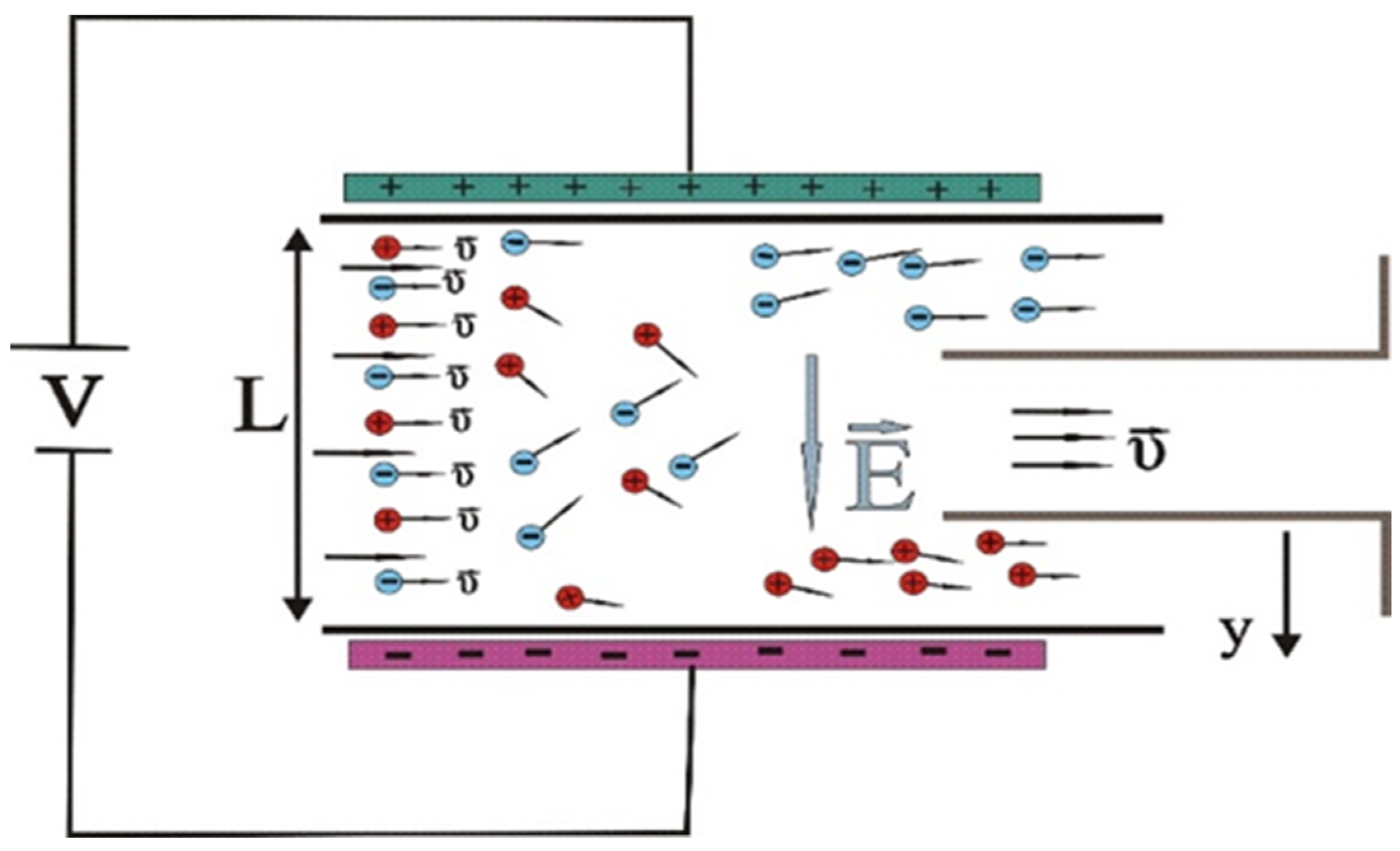
Two electrodes which are charged by V voltage, and which produce among themselves almost homogeneous electric field intensity with direction from positive to negative electrode.

(2)

An insulated duct in which the contaminated water flows through. This is placed along the electrodes and at the minimum distance from them to ensure that the external electric field is almost homogeneous. Therefore, the contaminated water with velocity $\overrightarrow{\upsilon }$ flows perpendicular to the external electric field intensity, which is considered along the y-axis (Figure 1 and Figure 2), and a change of the toxin ion concentration along the y-axis of the duct is observed (Figure 3).

Throughout the analysis that follows, water is considered as a continuous medium [23,24,25,26] with electric permittivity$\epsilon ={\epsilon }_r{\epsilon }_0$, where ${\epsilon }_r\approx 80$ is the relative permittivity of the water and ${\epsilon }_0=8.85\times {10}^{-12} \mathrm{F}/\mathrm{m}$.

3. Analysis of the Final Equilibrium State

3.1. Boundary Conditions

The main problem to deal with is the size of the toxin ions, which is huge compared to atomic ions. Moreover, these molecules are not compact, nor they have a defined shape. Therefore, the first assumption made is that these proteins are spheres with effective radius mentioned in Table 1. A second assumption considered is that, during their movement, toxin ions are not noticeably deformed, losing entirely their spherical shape. Consequently, the electric field applied should have a relatively small intensity. By considering them approximately spheres, their center cannot approach the duct wall at a distance less than their radius, so the Stern model can be used. According to this model, near to each electrode, a double layer is formed (the area that the ions are cornered) consisting of two parts [27,28]:

(a)

The compact part (Stern layer), which consists of one layer of ions in direct contact with the walls of the duct. This is simulated with a Helmholtz capacitor, as presented in Figure 4, with effective width ${\lambda }_S,$ approximately equal to the radius of the ion (Table 1). Thus, the capacity of the compact part per unit area $c_H$ is given by

$$c_H=\frac{\epsilon }{{\lambda }_S}$$

(1)

(b)

The diffuse layer, which is formed besides the compact part in the inner side of the duct which is simulated with a Gouy–Chapman-type capacitor with effective width $\lambda$(Figure 4) and capacity of the diffuse layer per unit area $c_D$ is given by

$$c_D=\frac{\epsilon }{\lambda }$$

(2)

Firstly, we should declare the boundary conditions. Considering that for $y=\frac{L}{2}$ (the center of the duct), the potential is equal to zero,$\phi \left(y=\frac{L}{2}\right)=0$.

Thus, the potential at the point with y = 0 is φ(0) and −φ(0) at y = L. Still, considering the relationship between potential and distance linear within the compact layer, we have:

$$\phi =\pm \phi \left(0\right)\pm {\lambda }_s\frac{\partial \phi }{\partial y} \mathrm{for} y=0,L$$

(3)

At this point, it should be clarified that in the model there is an external electric field which is created by the application of the voltage V on the two electrodes externally to the duct simultaneously with an opposite electric field which is created by the double layer of ions according to the Stern model. Therefore, the external electric field causes the movement of toxin ions and results in the creation within the solution of a total internal electric field. This internal electric field is mathematically expressed by the creation of potential φ (V), which varies spatially along the y axis.

3.2. Calculation of Final Equilibrium State

The intensity of the electric field inside the compact layer as well as the surface charge density $\sigma$ near positive or negative electrode is calculated, according to the method of Bartzis and Sarris [16]. Surface charge density (σ) is the amount of charge per unit of a two-dimensional surface area, and it is a measure of the quantity of electric charge accumulated over a surface. It is given by Equation (4):

$$\sigma =-\sqrt{8\epsilon C_{M}RT}\sinh [\frac{zF}{2RT}(\frac{\sigma {\lambda }_s}{\epsilon }+\phi \left(0\right))]$$

(4)

where $C_M$ is the toxin concentration at the middle of the duct after the electric potential application, T is the absolute temperature which is considered T = 300 K throughout the study, z is the number of overflow protons or electrons (considered positive throughout the article), $R=8.314\frac{\mathrm{J}}{\mathrm{mol}\cdot \mathrm{K}}$, and F = 96,485.34 C/mol is the Faraday constant.

We should at this point determine the $C_M$ which is the toxin concentration at the middle of the duct after the electric potential application and it is therefore a critical value because it expresses the amount of residual toxin after the treatment. In this model, this parameter ($C_M$) was set at a specific value, according to the maximum levels of the toxins in water that can be tolerated by a human. Since there is much scientific literature regarding the intoxication by staphylococcal toxins, in this model, the minimum tolerable level was considered as reference value for staphylococcal poisoning. Children will suffer staphylococcal food poisoning by ingesting as little as 100 ng of staphylococcal enterotoxins, and only a few micrograms of staphylococcal enterotoxins are enough to cause poisoning in vulnerable populations [29]. Assuming that ingestion of 50 mL of water containing 100 ng of the staphylococcal enterotoxins could be harmful to a child, the level of 2 ng/mL was selected as the target concentration to be achieved in our model and this value is the $C_M \left(\mathrm{accepted} \mathrm{limits} \mathrm{of} \mathrm{the} \mathrm{toxins}\right)$. Moreover, this level can be relatively easily quantified with existing analytical methods such as ELISA [29,30].

Taking into consideration the above reference value (2 ng/mL), the concentration of toxins$C_M$ (considered approximately as the “target” concentration in the area of the duct away from the double layer after the treatment of the electric field), expressed in $\raisebox{1ex}{$\mathrm{mol}$}\!\left/ \!\raisebox{-1ex}{${\mathrm{m}}^3$}\right.$, was calculated as following:

$$C_M=56\times {10}^{-9}\raisebox{1ex}{$\mathrm{mol}$}\!\left/ \!\raisebox{-1ex}{${\mathrm{m}}^3$}\right.$$

(5)

The calculation of the Equation (5) value was performed using the values of the first toxin and for simplicity reasons was considered constant for all four toxins. Figure 5 presents the surface charge density (the discrete points and not the lines which are explained in Section 4) as a function of $C_M$ for toxin 1 (Staphylococcus aureus alpha-hemolysin) for various $\phi \left(0\right)$ (as we have already mentioned, $\phi \left(0\right)$ is the potential applied to one side of the duct). It is observed that the surface charge density remains stable by increasing $C_M$. However, there is a large increase in surface charge density by increasing $\phi \left(0\right)$.

The electric field intensity inside the compact layer is given by Equation (6).

$${{\rm E}}_{{\lambda }_S}=-\frac{\sigma }{\epsilon }\to {{\rm E}}_{{\lambda }_S}=\sqrt{\frac{8C_{M}RT}{\epsilon }}\sinh [\frac{zF}{2RT}\left(-{\lambda }_s{{\rm E}}_{{\lambda }_S}+\phi \left(0\right)\right)]$$

(6)

but the same quantity outside the compact layer is described by Equation (7).

$$E=-\frac{\partial \phi }{\partial y}=\sqrt{\frac{8C_{M}RT}{\epsilon }}\sin \mathrm{h}\left(\frac{zF}{2RT}\phi \right)$$

(7)

where

$$\phi =\frac{4RT}{zF}{\mathit{tanh}}^{-1}\{\mathit{tanh}(\frac{zF{\phi }_s}{4RT})\cdot e^{-\kappa \left(y-{\lambda }_s\right)}\} \mathrm{for}\to {\lambda }_s\le y\le \raisebox{1ex}{$L$}\!\left/ \!\raisebox{-1ex}{$2$}\right.$$

(8)

and

$$\phi =\frac{4RT}{zF}{\mathit{tanh}}^{-1}\{-\mathit{tanh}(\frac{zF{\phi }_s}{4RT})\cdot e^{\kappa \left(y-L+{\lambda }_s\right)}\} \mathrm{for} \to \raisebox{1ex}{$L$}\!\left/ \!\raisebox{-1ex}{$2$}\right.\le y\le L-{\lambda }_s$$

(9)

where ${\lambda }_s$is replaced on a case-by-case basis (Table 1) and the potential ${\phi }_s$ at the outer Helmholtz plane (OHP) is related with $\phi \left(0\right)$ with Equation (10).

$${\phi }_S=\phi \left(0\right)-{\lambda }_s\sqrt{\frac{8C_{M}RT}{\epsilon }}\sinh (\frac{zF}{2RT}{\phi }_s)$$

(10)

In order to determine the area that is occupied by the excess of the charged toxins that were moved, and consequently the area of the liquid whose concentration is within acceptable limits, we must calculate the total differential capacitance $c_{tot}$, defined as

$$c_{tot}=\frac{\left|d\sigma \right|}{d\phi \left(0\right)}$$

Using Equation (4), we have:

$$c_{tot}=\frac{\sqrt{\frac{2C_M\epsilon z^2{F}^2}{RT}}\cos \mathrm{h}\left(\frac{zF}{2RT}{\phi }_s\right)}{1+\frac{{\lambda }_s}{\epsilon }\sqrt{\frac{2C_M\epsilon z^2{F}^2}{RT}}\cos \mathrm{h}\left(\frac{zF}{2RT}{\phi }_s\right)}$$

(11)

According to what has already been mentioned, the boundary layer consists of two capacitors connected in-line, the first corresponding to the compact layer (Stern layer) with capacity $c_H$and the second that to the diffuse layer with capacity $c_D$

$$c_H=\frac{\epsilon }{{\lambda }_s}$$

$$c_D=\sqrt{\frac{2C_M\epsilon z^2{F}^2}{RT}}\cos \mathrm{h}\left(\frac{zF}{2RT}{\phi }_s\right)$$

Moreover, $c_D$ can be alternatively expressed as:

$$c_D=\frac{\epsilon }{{\lambda }_D}\cos \mathrm{h}\left(\frac{zF}{2RT}{\phi }_s\right)$$

(12)

where

$${\lambda }_D={\kappa }^{-1}=\sqrt{\frac{\epsilon RT}{2z^2{C}_M{F}^2}}$$

(13)

is the diffuse layer width in the linear regime.

It is evident from Equation (12) that$c_D$depends on the initial concentration and the applied electric field. By using Equation (13), ${\lambda }_D$values for all toxins were calculated and are presented in

Table 2. Calculation of λ_D per toxin. λ_D: the diffuse layer width in the linear approximation which applies only when the applied potential is very small (it is a characteristic constant). C_M: the toxin concentration at the middle of the duct after the electric potential application.

	Toxin 1 Staphylococcus aureus, Alpha-Hemolysin	Toxin 2 Staphylococcus aureus, Toxic Shock Syndrome Toxin-1 (TSST-1)	Toxin 3 Staphylococcus aureus Enterotoxin Type A	Toxin 4 E. coli Shiga Toxin 2 (One Subunit A and Five Subunits B)
${\lambda }_D$ (m)	$1.79\times {10}^{-5}$	$1.71\times {10}^{-5}$	$3.51\times {10}^{-5}$	$5.41\times {10}^{-6}$
$C_M \left(\raisebox{1ex}{$\mathrm{mol}$}\!\left/ \!\raisebox{-1ex}{${\mathrm{m}}^3$}\right.\right)$	$56\times {10}^{-9}$

.

If $c_D$ is expressed as $c_D=\frac{\epsilon }{\lambda }$, where $\lambda$ represents the thickness of the effective capacitor of the diffuse layer, we can find the ratio:

$$\frac{\lambda }{{\lambda }_D}={\left[\cos \mathrm{h}\left(\frac{zF}{2RT}{\phi }_s\right)\right]}^{-1}$$

(14)

Figure 6 presents the change of $\frac{\lambda }{{\lambda }_D}$ as a function of$\phi \left(0\right)$ (Equation (13)) for $C_M=56\times {10}^{-9}\frac{\mathrm{mol}}{{\mathrm{m}}^3}$ for the different toxins.

As it is already mentioned, ${\lambda }_D$is the diffuse layer width in the linear regime, calculated for each toxin in Table 2. The physical significance of $\lambda$ is that it indicates the effective width of the area where the toxins are cornered with the application of the electric field. We should point out that our aim is to reduce λ as much as possible because this would mean that the toxins would be efficiently removed from the largest part of the duct. It is, therefore, evident that λ decreases with the increase in potential as well as with the increase in the charge of toxins. It is observed (Figure 6) that regarding the first and second toxins with z = 2.318 and z = 2.392 (red and green lines, respectively), for potential φ(0) = 0.1 V,$\frac{\lambda }{{\lambda }_D}$ is of order ${10}^{-2}.$Therefore, λ is two orders of magnitude smaller than ${\lambda }_D$(i.e., according to Table 2 $~{10}^{-7} \mathrm{m}$), for the third toxin with z = 1.176 (blue line) one order of magnitude smaller (i.e., $~{10}^{-6} \mathrm{m}$ ), whereas for the fourth toxin with z = 7.644 (black line) four orders of magnitude smaller (i.e.,$~{10}^{-10} \mathrm{m}$). This means that $\lambda$ is almost negligible compared to the L (total width of the duct) and it is considered at least $L~{10}^{-4} \mathrm{m}$. Conclusively, the largest part of the duct remains with the target toxin concentration $C_M,$ after the application of the electric field. Moreover, using a smaller width duct inside the larger duct in which the electric field is applied, the decontaminated solution can be collected, as previously presented in Figure 2.

Throughout the previous analysis, it is considered that the distribution of charged toxins along the duct follows the Boltzmann distribution. Obviously, this is true outside the compact layer. Moreover, there is symmetry at the two opposite electrodes. When the toxins are negatively charged (i.e., the distribution near the positively charged electrode), toxin concentration is expressed as:

$$C_{-}=C_M{e}^{+\frac{zF}{RT}\phi }$$

(15)

where potential φ is given by Equations (8) and (9). As already mentioned, $C_M$ is the concentration at the center of the duct after the application of the electric field and after the final equilibrium state has occurred. We consider it equal to the upper limit of the concentration we want to achieve, i.e.,

$$C_M=56\times {10}^{-9} \raisebox{1ex}{$\mathrm{mol}$}\!\left/ \!\raisebox{-1ex}{${\mathrm{m}}^3$}\right.$$

Let’s symbolize with $C_{bef}$ the uniform concentration of the toxin before applying the field. From the principle of the mass conservation, it can easily be derived that it is associated with the $C_M$ with the relationship:

$$C_{bef}=\frac{C_M{{\displaystyle \int }}_{{\lambda }_s}^{L-{\lambda }_s}{e}^{+\frac{zF}{RT}\phi }dy}{L}$$

or

$$\frac{C_M}{C_{bef}}=\frac{L}{{{\displaystyle \int }}_{{\lambda }_s}^{L-{\lambda }_s}{e}^{+\frac{zF}{RT}\phi }dy}$$

(16)

In Figure 7, Figure 8, Figure 9 and Figure 10 the fraction $\frac{C_M}{C_{bef}}$ is represented as a function of the width of the duct for various potentials for the four toxins with the desired final concentration $C_M=56\times {10}^{-9} \raisebox{1ex}{$\mathrm{mol}$}\!\left/ \!\raisebox{-1ex}{${\mathrm{m}}^3$}\right..$

Considering the numerator constant in the fraction $\frac{C_M}{C_{bef}}$, this becomes smaller the greater the concentration $C_{bef}$ is, before the application of the field. Therefore, the smaller this ratio becomes, the better results are achieved in terms of reducing the amount of initial toxin. From the Figure 7, Figure 8, Figure 9 and Figure 10, it is evident that the higher potential and the lower width of the duct decrease the ratio $\frac{C_M}{C_{bef}}.$

We observe in all graphs that, for the lowest value of potential $\phi \left(0\right)$ (V), we do not have a noticeable decrease in concentration (black lines). The lowest value of potentials in all diagrams represents the limit at which the linear approximation applies (the linear approximation is developed is Section 4). However, for potential ten times and twenty times larger than the lowest value, and for ducts less than 1 cm wide, the decrease in concentration of ion toxins in the main volume of the solution is enormous. Specifically, as we can see from the diagrams, for ducts with a width of 1 cm, the reduction is approximately 99% and for ducts with width 1 mm the reduction is approximately 99.9%. A further increase in the potential (a hundred times more than the lowest value) results in almost total elimination of the toxin in the main volume of the solution (blue lines). However, these results for the highest potential (blue lines) can only be qualitatively estimated because for these potentials the steric effects become significant, as we will see in the next paragraph.

3.3. Validity of the Model

In the above analysis, we considered that the concentration of ionized toxins follows the Boltzmann distribution in the final equilibrium state, i.e.,

$$C_{-}=C_M{e}^{+\frac{zF}{RT}\phi }$$

(17)

This assumes that the electrochemical potential obeys the relationship:

$$\tilde{\mu }={\mu }_0+RT ln{C}_{-}+ze\phi$$

(18)

which is true if the solution is dilute and the ions are considered as points (ideal solution). So, in our case, this equation is valid as long as the concentration is low and the toxin ions, although large in size, are still extremely far from each other. Of course, the approximation becomes the better the lower the concentration is.

Furthermore, the limitations posed by the fact that protein toxin ions have very large dimensions and are not point-based will be discussed. Let’s consider, on a case-by-case basis, that the toxin ions have the diameters mentioned in the

Table 3. Calculation of ${\phi }_s^{max}$ (the potential at the outer Helmholtz plane (OHP) when the concentration on it is$C_{max}$ ) and ${\phi }_{max}\left(0\right)$ (the corresponding potential applied to one side of the duct) per toxin.$C_{max}$: the maximum concentration that can be achieved due to steric effects and C_M: the toxin concentration at the middle of the duct after the electric potential application.

	Toxin 1 Staphylococcus aureus Alpha-Hemolysin	Toxin 2 Staphylococcus aureus Toxic Shock Syndrome Toxin-1 (TSST-1)	Toxin 3 Staphylococcus aureus Enterotoxin Type A	Toxin 4 E. coli Shiga Toxin 2 (One Subunit A and Five Subunits B)
$C_{max}$ ($\mathrm{mol}/{\mathrm{m}}^3$)	10.43	14.46	13.0	4.88
$C_M$($\mathrm{mol}/{\mathrm{m}}^3$)	$56\times {10}^{-9}$	$56\times {10}^{-9}$	$56\times {10}^{-9}$	$56\times {10}^{-9}$
${\phi }_s^{max}$(V)	0.21	0.22	0.41	0.062
${\phi }_{max}\left(0\right)$(V)	0.24	0.26	0.41	$0.082$

. The maximum concentration is reached where the Stern layer (compact layer) ends and the diffuse layer begins. This cannot be greater than [31]:

$$C_{max}=\frac{1}{N_A{a}^3}$$

(19)

The relationship that connects $C_{max}$ with ${\phi }_s^{max}$ prevailing at this point is

$$C_{max}=C_M{e}^{+\frac{zF}{RT}{\phi }_s^{max}}$$

So,

$${\phi }_s^{max}=\frac{RT}{zF}\ln \left(\frac{C_{max}}{C_M}\right)$$

(20)

while the corresponding ${\phi }_{max}\left(0\right)$is calculated from Equation (10) (${\phi }_{max}\left(0\right)$) is the maximum potential for which the above model is valid). All the above values are calculated on a case-by-case basis in Table 3. We cannot claim that the above values are more than indicative because of the approximations with which they were exported. However, again, the closer we get to ${\phi }_{max}\left(0\right),$the more the concentration of ions in OHP (Outer Helmholtz Plane) increases and approaches $C_{max},$ and the less the dilute solution approximation (Equation (18)) necessary for the Boltzmann distribution can be applied. Thus, referring to the previous analysis for potentials above 0.24 V for the first two toxins, 0.4 V for the third toxin, and 0.082 V for the fourth toxin, the results can be considered only qualitatively. However, given the extremely large reduction achieved in the concentration of toxins even with voltages of 0.24 V, 0.4 V, and 0.082 V, as we already mentioned, the further increase in voltage, although it cannot be supported by the model theoretically, in practice could result in a more efficient output (the blue lines of Figure 7, Figure 8, Figure 9 and Figure 10).

4. Estimation of Time in the Linear Approximation

One of the important parameters that should be examined in this theoretical model is the time required for the protein toxin drift to be achieved. This time can only be estimated by solving through the Poisson Nernst Planck equations (PNP Equations) in the linear regime, following the methodology developed in Ref. [16]. The linear approximation applies only when the applied potential is very small, i.e., when

$$\left|z\frac{\mathrm{F}}{\mathrm{RT}}\phi \left(0\right)\right|<1 \mathrm{or} z {\phi }_l^{max}\left(0\right)=0.026 \mathrm{V}$$

(21)

where ${\phi }_l^{max} \left(0\right)$ is the maximum potential for which the linear approximation applicable to the four ionized toxins is calculated in

Table 4. Calculation of toxin movement time $\frac{t_{tot}}{L}$ (completion time per unit width). ${\phi }_l^{max}\left(0\right)$: the maximum potential applied to one side of the duct for which the linear approximation holds, L: width of the duct.

	Toxin 1 Staphylococcus aureus Alpha-Hemolysin	Toxin 2 Staphylococcus aureus Toxic Shock Syndrome Toxin-1 (TSST-1)	Toxin 3 Staphylococcus aureus Enterotoxin Type A	Toxin 4 E. coli Shiga Toxin 2 (One Subunit A and Five Subunits B)
$\kappa ={\left[\sqrt{\frac{\epsilon RT}{2z^2{C}_M{F}^2}}\right]}^{-1}$ (m−1)	$56,324$	$58,122$	$28,575$	185,741
$L$ (m)	$\le {10}^{-2} \mathrm{m}$
${\lambda }_S$	$2.71\times {10}^{-9}$	$2.43\times {10}^{-9}$	$2.52\times {10}^{-9}$	$3.49\times {10}^{-9}$
${\phi }_l^{max}\left(0\right)=\left(\frac{RT}{zF}\right)$ (V)	$0.011$	$0.011$	$0.022$	0.003
$\frac{t_{tot}}{L}$ $\left(\raisebox{1ex}{$\mathrm{s}$}\!\left/ \!\raisebox{-1ex}{$\mathrm{mm}$}\right.\right)$	547	470	1000	210

.

Surface charge density in the linear regime ($\left|{\sigma }_l\right|)$according to Ref. [16] is given by the relationship

$$\left|{\sigma }_l\right|=\phi \left(0\right)\frac{\epsilon }{\left({\lambda }_S+{\kappa }^{-1}\right)}$$

(22)

where

$${\kappa }^{-1}={\lambda }_D=\sqrt{\frac{\epsilon RT}{2z^2{C}_M{F}^2}}$$

(23)

From Equation (22), the schematic representation of surface charge density as a function of $C_M$,($\left|{\sigma }_l\right|=f\left(C_M\right))$ in the linear regime is shown in Figure 5 with solid lines. We observe that the results of both the linear model (green line) and the exact calculation with the Stern model (blue points) coincide, as expected for low potentials, and diverge in higher potentials. This result confirms the correctness of our analysis since we expect the linear model to be valid only in low potentials and the Stern model analysis is valid and in higher potentials, as demonstrated in Section 3.3.

Regarding the estimation of time, the time constant is given by the relationship [16]

$$\tau =\frac{L\left(1+\frac{2{\lambda }_s}{L}\right)}{2D\kappa \left({\lambda }_s\kappa +\tanh \left(\kappa \frac{L}{2}\right)\right)}$$

(24)

In our case and for the values of ${\lambda }_s$ and $L$ that we are interested, shown in Table 4 (L is set less or equal ${10}^{-2} \mathrm{m}$, because according to Figure 7, Figure 8, Figure 9 and Figure 10 at this width we have the best efficiency of the model),

$$\frac{{\lambda }_s}{L}\le 3.5\times {10}^{-5}$$

(25)

and

$$\tanh \left(\kappa \frac{L}{2}\right)\approx 1$$

The time constant equation takes the form

$$\tau \cong \frac{L}{2D\kappa \left({\lambda }_s\kappa +1\right)}$$

(26)

As in all exponential quantities, the phenomenon is theoretically completed in infinite time, but in practice it has reached 99% of its final value in a time of 5τ. However, in time less than 5τ, e.g., 3τ, there is also significant reduction. It should be mentioned that:

(a)

The time constant in the linear regime as well as the completion time are proportional to the width of the duct. Therefore, it is useful to calculate the completion time per unit width (s/mm)

$$\frac{t_{tot}}{L}=\frac{5\tau }{L}=5·{\left[2D\kappa \left({\lambda }_s\kappa +1\right)\right]}^{-1}$$

(27)

and the results are represented in Table 4.

(b)

The values of the potential with which these times are achieved are extremely small (because only in very low potential the linear approximation can be satisfied)

(c)

Although we cannot predict time for higher potentials (as in our case), it is logical to assume that by increasing the external voltage, and consequently the potential φ(0), the time it takes for the bulk solution to reach acceptable concentration values will be drastically reduced.

5. Conclusions

Bacterial protein toxins are secreted by foodborne pathogens and represent a significant threat to public health. These toxins can be present in various environments, such as food matrices or water, even after the microorganism has been destroyed after thermal or other processes. Moreover, they are large biomolecules that remain stable to chemical inactivation and are generally resistant to extreme conditions, such as low pH, freezing, and drying. All proteins form in aqueous solution ions, positively and negatively charged, which are carried by ionizable groups in the amino acid residues. The theoretical model presented in this study describes the removal of four specific bacterial toxins from water by drifting after the application of an electric field. Here, it should be mentioned that two basic assumptions were made: (a) the spherical shape of the toxins and (b) the solution contains only toxins in a low concentration. In this theoretical analysis, the solution is considered as containing only toxins in a low concentration in order to study the behavior of charged protein toxins under the influence of an electric field. The analysis evaluates whether there is primary evidence of drift based on this hypothesis (there are only toxins present) because there is also a possibility that no drift is observed due to their relatively large size. The outcome of the analysis revealed that not only can drift be observed, but also that almost complete purification of toxins can be achieved, even in the application of very low voltages. More specifically, the results presented in this study are very encouraging for the application of the above method as a future tool for the removal from aqueous solutions of bacterial toxins, such as the three Staphylococcus aureus toxins, which have a total positive charge, and the Stx2 toxin of a STEC strain of Escherichia coli, which has a total negative charge and is much larger than the other three since it is an AB₅ hexamer. For a duct width of 1cm or less and for low applied potentials (0.1–0.4 V), a reduction up to 99% in the concentration of toxins was achieved in the main volume of the solution (which is the major part of the duct width) for target concentration $56\times {10}^{-9} \raisebox{1ex}{$\mathrm{mol}$}\!\left/ \!\raisebox{-1ex}{${\mathrm{m}}^3$}\right.$. Therefore, acceptable toxin concentrations can be achieved from solutions a hundred times more contaminated, and this makes the method applicable to pre-purified solutions and for small-scale water decontamination.

In practice, of course, usually, the contaminated water may also contain other impurities, some of which are in ionic form (which create resistivity). Consequently, they will also be affected by the electric field and will move accordingly, some of them faster than the toxins, polarizing the electrodes [16,17,18] and preventing the drift of toxins. For this reason, purification of the contaminated water with other methods should have preceded in order to remove most of the pollutants. According to the theoretical analysis, the method can provide a solution to the removal of toxins from already purified solutions which have low concentrations of toxins but remain capable of causing harm to health and which cannot be removed by primary treatment. Due to the very encouraging results, a future study analyzing the drift of toxins in the presence of other ionic pollutants and with the application of higher voltages would contribute further to the development of an effective model.

References

1. Rajkovic, A.; Jovanovic, J.; Monteiro, S.; Decleer, M.; Andjelkovic, M.; Foubert, A.; Beloglazova, N.; Tsilla, V.; Sas, B.; Madder, A.; et al. Detection of Toxins Involved in Foodborne Diseases Caused by Gram-Positive Bacteria. Compr. Rev. Food Sci. Food Saf. 2020, 19, 1605–1657. [Google Scholar] [CrossRef] [PubMed]
2. Abril, A.G.; Villa, T.G.; Barros-Velázquez, J.; Cañas, B.; Sánchez-Pérez, A.; Calo-Mata, P.; Carrera, M. Staphylococcus Aureus Exotoxins and Their Detection in the Dairy Industry and Mastitis. Toxins 2020, 12, 537. [Google Scholar] [CrossRef] [PubMed]
3. Amirsoleimani, A.; Brion, G.M.; Diene, S.M.; François, P.; Richard, E.M. Prevalence and Characterization of Staphylococcus Aureus in Wastewater Treatment Plants by Whole Genomic Sequencing. Water Res. 2019, 158, 193–202. [Google Scholar] [CrossRef] [PubMed]
4. Silva, V.; Ferreira, E.; Manageiro, V.; Reis, L.; Tejedor-Junco, M.T.; Sampaio, A.; Capelo, J.L.; Caniça, M.; Igrejas, G.; Poeta, P. Distribution and Clonal Diversity of Staphylococcus Aureus and Other Staphylococci in Surface Waters: Detection of ST425-T742 and ST130-T843 MecC-Positive MRSA Strains. Antibiotics 2021, 10, 1416. [Google Scholar] [CrossRef]
5. Silva, V.; Caniça, M.; Capelo, J.L.; Igrejas, G.; Poeta, P. Diversity and Genetic Lineages of Environmental Staphylococci: A Surface Water Overview. FEMS Microbiol. Ecol. 2020, 96, fiaa191. [Google Scholar] [CrossRef]
6. Vandenesch, F.; Lina, G.; Henry, T. Staphylococcus Aureus Hemolysins, Bi-Component Leukocidins, and Cytolytic Peptides: A Redundant Arsenal of Membrane-Damaging Virulence Factors? Front. Cell. Infect. Microbiol. 2012, 2, 12. [Google Scholar] [CrossRef] [Green Version]
7. Oliveira, D.; Borges, A.; Simões, M. Staphylococcus Aureus Toxins and Their Molecular Activity in Infectious Diseases. Toxins 2018, 10, 252. [Google Scholar] [CrossRef] [Green Version]
8. Dinges, M.M.; Orwin, P.M.; Schlievert, P.M.; Biology, S.; The, O.F. Exotoxins of Staphylococcus Aureus. Clin. Microbiol. Rev. Jan. 2000, 13, 16–34. [Google Scholar] [CrossRef]
9. Sugawara, T.; Yamashita, D.; Kato, K.; Peng, Z.; Ueda, J.; Kaneko, J.; Kamio, Y.; Tanaka, Y.; Yao, M. Structural Basis for Pore-Forming Mechanism of Staphylococcal α-Hemolysin. Toxicon 2015, 108, 226–231. [Google Scholar] [CrossRef] [Green Version]
10. Gonzalez, A.G.M.; Cerqueira, A.M.F.; Guth, B.E.C.; Coutinho, C.A.; Liberal, M.H.T.; Souza, R.M.; Andrade, J.R.C. Serotypes, Virulence Markers and Cell Invasion Ability of Shiga Toxin-Producing Escherichia Coli Strains Isolated from Healthy Dairy Cattle. J. Appl. Microbiol. 2016, 121, 1130–1143. [Google Scholar] [CrossRef]
11. Joseph, A.; Cointe, A.; Mariani Kurkdjian, P.; Rafat, C.; Hertig, A. Shiga Toxin-Associated Hemolytic Uremic Syndrome: A Narrative Review. Toxins 2020, 12, 67. [Google Scholar] [CrossRef] [PubMed] [Green Version]
12. Keir, L.S. Shiga Toxin Associated Hemolytic Uremic Syndrome. Hematol. Oncol. Clin. N. Am. 2015, 29, 525–539. [Google Scholar] [CrossRef] [PubMed]
13. Siegler, R.L.; Obrig, T.G.; Pysher, T.J.; Tesh, V.L.; Denkers, N.D.; Taylor, F.B. Response to Shiga Toxin 1 and 2 in a Baboon Model of Hemolytic Uremic Syndrome. Pediatr. Nephrol. 2003, 18, 92–96. [Google Scholar] [CrossRef] [PubMed]
14. Touchon, M.; Cury, J.; Yoon, E.J.; Krizova, L.; Cerqueira, G.C.; Murphy, C.; Feldgarden, M.; Wortman, J.; Clermont, D.; Lambert, T.; et al. The Genomic Diversification of the Whole Acinetobacter Genus: Origins, Mechanisms, and Consequences. Genome Biol. Evol. 2014, 6, 2866–2882. [Google Scholar] [CrossRef] [PubMed] [Green Version]
15. Conrady, D.G.; Flagler, M.J.; Friedmann, D.R.; Vander Wielen, B.D.; Kovall, R.A.; Weiss, A.A.; Herr, A.B. Molecular Basis of Differential B-Pentamer Stability of Shiga Toxins 1 and 2. PLoS ONE 2010, 5, e15153. [Google Scholar] [CrossRef] [Green Version]
16. Bartzis, V.; Sarris, I.E. Time Evolution Study of the Electric Field Distribution and Charge Density Due to Ion Movement in Salty Water. Water 2021, 13, 2185. [Google Scholar] [CrossRef]
17. Bartzis, V.; Sarris, I.E. A Theoretical Model for Salt Ion Drift Due to Electric Field Suitable to Seawater Desalination. Desalination 2020, 473, 114163. [Google Scholar] [CrossRef]
18. Bartzis, V.; Sarris, I.E. Electric Field Distribution and Diffuse Layer Thickness Study Due to Salt Ion Movement in Water Desalination. Desalination 2020, 490, 114549. [Google Scholar] [CrossRef]
19. Sofos, F.; Karakasidis, T.E.; Spetsiotis, D. Molecular Dynamics Simulations of Ion Separation in Nano-Channel Water Flows Using an Electric Field. Mol. Simul. 2019, 45, 1395–1402. [Google Scholar] [CrossRef]
20. Sofos, F.; Karakasidis, T.E.; Sarris, I.E. Effects of Channel Size, Wall Wettability, and Electric Field Strength on Ion Removal from Water in Nanochannels. Sci. Rep. 2022, 12, 641. [Google Scholar] [CrossRef]
21. Sofos, F. A Water/Ion Separation Device: Theoretical and Numerical Investigation. Appl. Sci. 2021, 11, 8548. [Google Scholar] [CrossRef]
22. Fischer, H.; Polikarpov, I.; Craievich, A.F. Average Protein Density Is a Molecular-Weight-Dependent Function. Protein Sci. 2009, 13, 2825–2828. [Google Scholar] [CrossRef] [PubMed]
23. Atkins, P.; Paola, J. Atkin’s Physical Chemistry; Oxford University Press: Oxford, UK, 2006. [Google Scholar]
24. Mortimer, R.G. Physical Chemistry; John Wiley & Sons: New York, UY, USA, 2008; Volume 8. [Google Scholar]
25. Brett, C.M.A.; Brett, A.M.O. Electrochemistry Principles, Methods, and Applications; Oxford University Press: Oxford, UK, 1994. [Google Scholar]
26. Debye, P.; Hückel, E. The Theory of Electrolytes. I. Lowering of Freezing Point and Related Phenomena. Phys. Z. 1923, 24, 185–206. [Google Scholar]
27. Bonnefont, A.; Argoul, F.; Bazant, M. Analysis of Diffuse Layer on Time-Dependent Interfacial Kinetics. J. Electroanal. Chem. 2001, 500, 52. [Google Scholar] [CrossRef]
28. Bazant, M.Z.; Thornton, K.; Ajdari, A. Diffuse-Charge Dynamics in Electrochemical Systems. Phys. Rev. E Stat. Phys. Plasmas Fluids Relat. Interdiscip. Top. 2004, 70, 24. [Google Scholar] [CrossRef] [Green Version]
29. Wu, S.; Duan, N.; Gu, H.; Hao, L.; Ye, H.; Gong, W.; Wang, Z. A Review of the Methods for Detection of Staphylococcus Aureus Enterotoxins. Toxins 2016, 8, 176. [Google Scholar] [CrossRef] [Green Version]
30. Aguilar, J.L.; Varshney, A.K.; Wang, X.; Stanford, L.; Scharff, M.; Fries, B.C. Detection and Measurement of Staphylococcal Enterotoxin-like K (SEl-K) Secretion by Staphylococcus Aureus Clinical Isolates. J. Clin. Microbiol. 2014, 52, 2536–2543. [Google Scholar] [CrossRef] [Green Version]
31. Kilic, M.S.; Bazant, M.Z.; Ajdari, A. Steric Effects in the Dynamics of Electrolytes at Large Applied Voltages. I. Double-Layer Charging. Phys. Rev. E Stat. Nonlinear Soft Matter Phys. 2007, 75, 021502. [Google Scholar] [CrossRef] [Green Version]
32. Wellcome Sanger Institute. Toxic Shock Syndrome Toxin-1 [Staphylococcus Aureus]; Wellcome Sanger Institute: Hinxton, UK, 2020. Available online: https://www.ncbi.nlm.nih.gov/protein/CAC5806749.1 (accessed on 1 October 2022).
33. Zhang, Y.; Liao, Y.-T.; Salvador, A.; Sun, X.; Wu, V. Complete Genome Sequence of a Shiga Toxin-Converting Bacteriophage, Escherichia Phage Lys12581Vzw, Induced from an Outbreak Shiga Toxin-Producing Escherichia coli. Microbiol. Resour. Announc. 2020, 8, e00793-19. [Google Scholar] [CrossRef]
Figure 1. Configuration of the toxin drift model (V: voltage of the electrodes, L: width of the duct, E: electric field intensity, υ : velocity of contaminated water). The electrodes of the capacitor that create the electric field between them are represented as well as the duct with the contaminated water flowing inside it perpendicular to the electric field intensity.
Applsci 12 12739 g001
Figure 2. Configuration of ion toxin movement through the duct. (V: voltage of the electrodes; L: width of the duct, E: electric field intensity, υ : velocity of ions). Due to the electric field created by the electrodes, the ions according to their charge accumulate on both sides of the duct.
Applsci 12 12739 g002
Figure 3. Change of toxin concentration C+ across the duct width L, supposing that it has positive charge. CM: the toxin concentration at the middle of the duct after the electric potential application. The top illustration represents the duct after applying the electric field showing the accumulation of charged toxins on one side of it.
Applsci 12 12739 g003
Figure 4. Configuration of the double layer and equivalent capacitor representation, OHP: Outer Helmholtz Plane.
Applsci 12 12739 g004
Figure 5. Surface charge density | σ |   ( C m 2 )   as a function of C M   ( mol m 3 ) for toxin 1 (Staphylococcus aureus alpha-hemolysin) for various electric potentials φ ( 0 )   ( V ) (discrete points). Solid lines represent the corresponding | σ l | values.
Applsci 12 12739 g005
Figure 6. Ratio of   λ λ D for all the toxins as a function of φ ( 0 ) (V) for C M = 56 × 10 9 mol m 3 .
Applsci 12 12739 g006
Figure 7. C M C b e f as a function of L (m) for toxin 1, concentration C M = 56 × 10 9 mol m 3 for various potentials φ ( 0 ) (V).
Applsci 12 12739 g007
Figure 8. C M C b e f as a function of L (m) for toxin 2, concentration C M = 56 × 10 9 mol m 3 for various potentials φ ( 0 ) (V).
Applsci 12 12739 g008
Figure 9. C M C b e f as a function of L (m) for toxin 3, concentration C M = 56 × 10 9 mol m 3 for various potentials φ ( 0 ) (V).
Applsci 12 12739 g009
Figure 10. C M C b e f as a function of L (m) for toxin 4, concentration C M = 56 × 10 9 mol m 3 for various potentials φ ( 0 ) (V).
Applsci 12 12739 g010