Parameter Estimation for Some Probability Distributions Used in Hydrology

Abstract

Estimating the parameters of probability distributions generally involves solving a system of nonlinear equations or a nonlinear equation, being a technical difficulty in their usual application in hydrology. The choice of probability distributions for the calculation of extreme values in hydrology is, in most cases, made according to the ease of calculation of the estimated parameters and the explicit form of the inverse probability function. This article presents improved approximations and, in some cases, new approximations for the estimation with the method of ordinary moments and the method of linear moments, which are useful for the direct calculation of the parameters, because the errors in the approximate estimation are similar to the use of iterative numerical methods. Thirteen probability distributions of two and three parameters frequently used in hydrology are presented, for which parameter estimation was laborious. Thus, the approximate estimation of the parameters by the two methods is simple but also precise and easily applicable by hydrology researchers. The new and improved approximate forms presented in this article are the result of the research conducted within the Faculty of Hydrotechnics to update the Romanian normative standards in the hydrotechnical field.

1. Introduction

Probability distributions are used in hydrology to determine the probability of occurrence of extreme events: maximum flows, maximum volumes and maximum precipitation.

A criticism of the probabilistic estimation of extreme events is that it does not take climate changes into account, this being generally solved with hydrological modeling using learning machines [1] of the neural network type and others. However, statistical modeling is complementary and necessary to other types of black-box and gray-box modeling, because the input and output data from these models must be presented probabilistically, especially for extreme events with low probability, necessary for the design of hydrotechnical constructions.

In the case of determining the maximum flows, three or more parameter distributions are recommended, while for the determination of precipitation and maximum volumes, two parameter distributions are recommended [2,3,4].

In general, finding approximate relations to express the parameters is very important because many of these probability distributions, for exact determination, require solving with the Levenberg–Marquardt algorithm [5] for nonlinear least squares curve-fitting problems, which can sometimes represent a difficulty requiring the use of specific calculation programs.

Another important aspect is the expression of the quantile function (inverse of the distribution function) of these distributions, both of which facilitate the use of these distributions in the determination of the analyzed extreme values.

This article presents approximate forms of the expressions of some parameters of some frequently used probability distributions in hydrology, such as: Pearson III (PE3), Generalized extreme value (GEV), Weibull (W3), Weibull (W2), Fréchet (F3), Fréchet (F2), Generalized Pareto (P3), Log-Logistics (LG3), Kappa (K3-Generalized Gumbel), Kappa (K3-Park), Pearson V (PV3), Pearson V (PV2) and Generalized Exponential (EG2).

The approximate forms are for determining the parameters using the method of ordinary moments (MOM) and the method of linear moments (L-moments).

For the method of ordinary moments, the parameters of the three-parameter distributions are determined from relationships that use mean, variance and skewness, the latter representing the ratio between the centered moment of order 3 and variance to the 1.5 power. For the method of linear moments, the parameters of the distribution are determined from relations that use the arithmetic mean (${\mathrm{L}}_1$), ${\mathrm{L}}_2$ and ${\mathrm{\tau }}_3$, the latter representing the ratio between the moment ${\mathrm{L}}_3$ and ${\mathrm{L}}_2$.

These methods are some of the most frequently used methods for estimating parameters in hydrology [2,3,4,6,7,8,9]. The approximations use rational and polynomial functions in which the coefficients are obtained by least squares nonlinear regression on the domain of definition considered.

In some cases, the approach is similar by using the same type of function but with more terms, and in other cases the approach is different by using other types of functions.

For the method of ordinary moments, the approximation range most often used for skewness is 0–4, but in certain regions of the world they meet up to a skewness equal to 9 [3], or the skewness is adopted by multiplying the coefficient of variation with a chosen positive coefficient [10], so the skewness is always positive, even if that of the given sample may have negative skewness values. The definition range of approximations 0–8 was chosen in the case of MOM, and the definition range for the method of linear moments is the default 0–1. Considering that the approximation relations must be as accurate as possible, the relative error graphs are also presented. The relative error is the ratio between the difference between the exact and approximate value of the skewness, and the exact value. In this article, the new approximation relations are noted as “a better approximation”. For the L-skewness of the sample, it can have negative values, generally greater than −0.4.

Thus, all these novelty elements for these distributions presented in Table 1 will help hydrology researchers to use these distributions easily.

Table 1. Novelty elements.

Approximations	MOM	L-Moments
A better approximation	GEV, LL3	PE3, GEV, F3
A new approximation	W3, W2, F3, F2, P3, K3, PV3, EG2	W3, K3, PV3, PV2, EG2

The research also had as its object the use of mathematics by the large mass of engineers in the field of hydrotechnics, because the use of dedicated software without knowledge of mathematical methods is not beneficial. In this way, functions from Mathcad were presented comparatively, which can be equated by researchers with functions from their favorite programs (Matlab, Excel, Python, R, etc.).

2. Probability Distributions

In this section, the analyzed probability distributions are presented. The probability density function, $\mathrm{f}\left(\mathrm{x}\right)$; the complementary cumulative distribution function, $\mathrm{F}\left(\mathrm{x}\right)$, and quantile function (inverse function), $\mathrm{x}\left(\mathrm{p}\right)$ are presented below.

2.1. Pearson III Distribution (PE3)

The Pearson III distribution belongs to the Gamma distribution family, being a generalized form of the two-parameter Gamma distribution [11], with shifted $\mathrm{x}$, and a particular case of the four-parameter gamma distribution [5,12,13].

$$\mathrm{f}\left(\mathrm{x}\right)=\frac{{\left(\mathrm{x}-\mathrm{\gamma }\right)}^{\mathsf{\alpha }-1}}{{\mathsf{\beta }}^{\mathsf{\alpha }}·\mathrm{\Gamma }\left(\mathsf{\alpha }\right)}·\exp \left(-\frac{\mathrm{x}-\mathrm{\gamma }}{\mathsf{\beta }}\right)=\frac{1}{\mathsf{\beta }}·\mathrm{d}\mathrm{g}\mathrm{a}\mathrm{m}\mathrm{m}\mathrm{a}\left(\frac{\mathrm{x}-\mathrm{\gamma }}{\mathsf{\beta }},\mathsf{\alpha }\right)$$

(1)

$$\mathrm{F}\left(\mathrm{x}\right)=1-{\displaystyle \underset{\mathrm{\gamma }}{\overset{\mathrm{x}}{\int }}\mathrm{f}\left(\mathrm{x}\right)}\mathrm{d}\mathrm{x}=1-\frac{1}{\mathsf{\beta }·\mathrm{\Gamma }\left(\mathsf{\alpha }\right)}·{{\displaystyle \underset{\mathrm{\gamma }}{\overset{\mathrm{x}}{\int }}\left(\frac{\mathrm{x}-\mathrm{\gamma }}{\mathsf{\beta }}\right)}}^{\mathsf{\alpha }-1}·\exp \left(-\frac{\mathrm{x}-\mathrm{\gamma }}{\mathsf{\beta }}\right)\mathrm{d}\mathrm{x}=\frac{\mathrm{\Gamma }\left(\mathsf{\alpha },\frac{\mathrm{x}-\mathrm{\gamma }}{\mathsf{\beta }}\right)}{\mathrm{\Gamma }\left(\mathsf{\alpha }\right)}$$

(2)

$$\mathrm{F}\left(\mathrm{x}\right)=1-\mathrm{p}\mathrm{g}\mathrm{a}\mathrm{m}\mathrm{m}\mathrm{a}\left(\frac{\mathrm{x}-\mathrm{\gamma }}{\mathsf{\beta }},\mathsf{\alpha }\right)=1-\mathrm{p}\mathrm{c}\mathrm{h}\mathrm{i}\mathrm{s}\mathrm{q}\left(2·\frac{\mathrm{x}-\mathrm{\gamma }}{\mathsf{\beta }},2·\mathsf{\alpha }\right)$$

(3)

$$\mathrm{x}\left(\mathrm{p}\right)={\mathrm{F}}^{-1}\left(\mathrm{x}\right)=\mathrm{\gamma }+\mathsf{\beta }·{\mathrm{\Gamma }}^{ -1}\left(1-\mathrm{p};\mathsf{\alpha }\right)=\mathrm{\gamma }+\mathsf{\beta }·\mathrm{q}\mathrm{g}\mathrm{a}\mathrm{m}\mathrm{m}\mathrm{a}\left(1-\mathrm{p},\mathsf{\alpha }\right)$$

(4)

where $\mathsf{\alpha },\mathsf{\beta },\mathrm{\gamma }$ are the shape, the scale and the position parameters and $\mathrm{x}$ can take any values of range $\mathrm{\gamma }<\mathrm{x}<\infty$ if $\mathsf{\beta }>0$ or $-\infty <\mathrm{x}<\mathrm{\gamma }$ if $\mathsf{\beta }<0$ and $\mathsf{\alpha }>0$; $\mathsf{\mu },\mathrm{\sigma }$ represent the mean (expected value) and standard deviation. If $\mathsf{\beta }<0$ (negative skewness) then the first argument of the inverse of the distribution function Gamma, ${\mathrm{\Gamma }}^{ -1}\left(1-\mathrm{p};\mathsf{\alpha }\right)$ becomes ${\mathrm{\Gamma }}^{ -1}\left(\mathrm{p};\mathsf{\alpha }\right)$.

The expressions of the inverse function $\mathrm{x}\left(\mathrm{p}\right)={\mathrm{F}}^{-1}\left(\mathrm{x}\right)$, using the mean and standard deviation, are valid only for the method of ordinary moments.

2.2. Generalized Extreme Value Distribution (GEV)

The GEV distribution was introduced for the first time by Jenkins in 1955 [11] for the analysis of extreme values. It is also known as the Fisher–Tippett distribution.

Depending on the sign of the shape parameter, this can be transformed into the Weibull ($\mathsf{\alpha }<0$), Fréchet ($\mathsf{\alpha }>0$) or Gumbel ($\mathsf{\alpha }=0$) distributions [11,13,14].

$$\mathrm{f}\left(\mathrm{x}\right)={\left(1-\frac{\mathsf{\alpha }}{\mathsf{\beta }}·\left(\mathrm{x}-\mathrm{\gamma }\right)\right)}^{\frac{1}{\mathsf{\alpha }}-1}·\frac{1}{\mathsf{\beta }}·\exp \left(-{\left(1-\frac{\mathsf{\alpha }}{\mathsf{\beta }}·\left(\mathrm{x}-\mathrm{\gamma }\right)\right)}^{\frac{1}{\mathsf{\alpha }}}\right)$$

(5)

$$\mathrm{F}\left(\mathrm{x}\right)=1-\exp \left(-{\left(1-\frac{\mathsf{\alpha }}{\mathsf{\beta }}·\left(\mathrm{x}-\mathrm{\gamma }\right)\right)}^{\frac{1}{\mathsf{\alpha }}}\right)$$

(6)

$$\mathrm{x}\left(\mathrm{p}\right)=\mathrm{\gamma }+\frac{\mathsf{\beta }}{\mathsf{\alpha }}·\left(1-{\left(-\ln \left(1-\mathrm{p}\right)\right)}^{\mathsf{\alpha }}\right)$$

(7)

where $\mathsf{\alpha },\mathsf{\beta },\mathrm{\gamma }$ are the shape, the scale and the position parameters; $\mathrm{x}$ can take any values of range $\mathrm{x}<\left(\mathrm{\gamma }+\frac{\mathsf{\beta }}{\mathsf{\alpha }}\right)$ if $\mathsf{\alpha }>0$, and $\mathrm{x}>\left(\mathrm{\gamma }+\frac{\mathsf{\beta }}{\mathsf{\alpha }}\right)$ if $\mathsf{\alpha }<0$.

2.3. Weibull Distribution (W3)

The distribution represents a particular case of the GEV distribution when the shape parameter is negative. It is also known as the Type II extreme value distribution, [11,15,16].

$$\mathrm{f}\left(\mathrm{x}\right)=\frac{\mathsf{\alpha }}{\mathsf{\beta }}·{\left(\frac{\mathrm{x}-\mathrm{\gamma }}{\mathsf{\beta }}\right)}^{\mathsf{\alpha }-1}·{\mathrm{e}}^{-{\left(\frac{\mathrm{x}-\mathrm{\gamma }}{\mathsf{\beta }}\right)}^{\mathsf{\alpha }}}=\frac{\mathsf{\alpha }}{\mathsf{\beta }}·\mathrm{d}\mathrm{w}\mathrm{e}\mathrm{i}\mathrm{b}\mathrm{u}\mathrm{l}\mathrm{l}\left(\frac{\mathrm{x}-\mathrm{\gamma }}{\mathsf{\beta }},\mathsf{\alpha }\right)$$

(8)

$$\mathrm{F}\left(\mathrm{x}\right)={\mathrm{e}}^{-{\left(\frac{\mathrm{x}-\mathrm{\gamma }}{\mathsf{\beta }}\right)}^{\mathsf{\alpha }}}=1-\mathrm{p}\mathrm{w}\mathrm{e}\mathrm{i}\mathrm{b}\mathrm{u}\mathrm{l}\mathrm{l}\left(\frac{\mathrm{x}-\mathrm{\gamma }}{\mathsf{\beta }},\mathsf{\alpha }\right)$$

(9)

$$\mathrm{x}\left(\mathrm{p}\right)=\mathrm{\gamma }+\mathsf{\beta }·{\left(-\ln \left(\mathrm{p}\right)\right)}^{1/\mathsf{\alpha }}=\mathrm{\gamma }+\mathsf{\beta }·\mathrm{q}\mathrm{w}\mathrm{e}\mathrm{i}\mathrm{b}\mathrm{u}\mathrm{l}\mathrm{l}\left(1-\mathrm{p},\mathsf{\alpha }\right)$$

(10)

where $\mathsf{\alpha },\mathsf{\beta },\mathrm{\gamma }$ are the shape, the scale and the position parameters; $\mathsf{\alpha },\mathsf{\beta }>0,\mathrm{x}\ge \mathrm{\gamma }$.

2.4. Weibull Distribution (W2)

The distribution represents a particular case of the W3 distribution when the position parameter is 0 [11,16]:

$$\mathrm{f}\left(\mathrm{x}\right)=\frac{\mathsf{\alpha }}{\mathsf{\beta }}·{\left(\frac{\mathrm{x}}{\mathsf{\beta }}\right)}^{\mathsf{\alpha }-1}·\exp \left(-{\left(\frac{\mathrm{x}}{\mathsf{\beta }}\right)}^{\mathsf{\alpha }}\right)=\frac{1}{\mathsf{\beta }}·\mathrm{d}\mathrm{w}\mathrm{e}\mathrm{i}\mathrm{b}\mathrm{u}\mathrm{l}\mathrm{l}\left(\frac{\mathrm{x}}{\mathsf{\beta }},\mathsf{\alpha }\right)$$

(11)

$$\mathrm{F}\left(\mathrm{x}\right)=\exp \left(-{\left(\frac{\mathrm{x}}{\mathsf{\beta }}\right)}^{\mathsf{\alpha }}\right)=1-\mathrm{p}\mathrm{w}\mathrm{e}\mathrm{i}\mathrm{b}\mathrm{u}\mathrm{l}\mathrm{l}\left(\frac{\mathrm{x}}{\mathsf{\beta }},\mathsf{\alpha }\right)$$

(12)

$$\mathrm{x}\left(\mathrm{p}\right)=\mathsf{\beta }·{\left(-\ln \left(\mathrm{p}\right)\right)}^{1/\mathsf{\alpha }}=\mathsf{\beta }·\mathrm{q}\mathrm{w}\mathrm{e}\mathrm{i}\mathrm{b}\mathrm{u}\mathrm{l}\mathrm{l}\left(1-\mathrm{p},\mathsf{\alpha }\right)$$

(13)

where $\mathsf{\alpha },\mathsf{\beta }$ are the shape and the scale parameters; $\mathsf{\alpha },\mathsf{\beta },\mathrm{x}>0$.

2.5. Fréchet Distribution (F3)

The distribution represents a particular case of the GEV distribution when the shape parameter is positive. It is also known as the Type III extreme value distribution [11,17,18].

$$\mathrm{f}\left(\mathrm{x}\right)=\frac{\mathsf{\alpha }}{\mathsf{\beta }}·{\left(\frac{\mathrm{x}-\mathrm{\gamma }}{\mathsf{\beta }}\right)}^{-\mathsf{\alpha }-1}·\exp \left(-{\left(\frac{\mathrm{x}-\mathrm{\gamma }}{\mathsf{\beta }}\right)}^{-\mathsf{\alpha }}\right)$$

(14)

$$\mathrm{F}\left(\mathrm{x}\right)=1-\exp \left(-{\left(\frac{\mathrm{x}-\mathrm{\gamma }}{\mathsf{\beta }}\right)}^{-\mathsf{\alpha }}\right)$$

(15)

$$\mathrm{x}\left(\mathrm{p}\right)=\mathrm{\gamma }+\mathsf{\beta }·{\left(-\ln \left(1-\mathrm{p}\right)\right)}^{-1/\mathsf{\alpha }}$$

(16)

where $\mathsf{\alpha },\mathsf{\beta },\mathrm{\gamma }$ are the shape, the scale and the position parameters; $\mathsf{\alpha },\mathsf{\beta }>0,-\infty <\mathrm{\gamma }<\infty ,\mathrm{x}>\mathrm{\gamma }$.

2.6. Fréchet Distribution (F2)

The distribution represents a particular case of the F3 distribution when the position parameter is 0 [16].

$$\mathrm{f}\left(\mathrm{x}\right)=\frac{\mathsf{\alpha }}{\mathsf{\beta }}·{\left(\frac{\mathsf{\beta }}{\mathrm{x}}\right)}^{\mathsf{\alpha }+1}·\exp \left(-{\left(\frac{\mathsf{\beta }}{\mathrm{x}}\right)}^{\mathsf{\alpha }}\right)$$

(17)

$$\mathrm{F}\left(\mathrm{x}\right)=1-\exp \left(-{\left(\frac{\mathsf{\beta }}{\mathrm{x}}\right)}^{\mathsf{\alpha }}\right)$$

(18)

$$\mathrm{x}\left(\mathrm{p}\right)=\mathsf{\beta }·{\left(-\ln \left(1-\mathrm{p}\right)\right)}^{-1/\mathsf{\alpha }}$$

(19)

where $\mathsf{\alpha },\mathsf{\beta }$ are the shape and the scale parameters; $\mathsf{\alpha },\mathsf{\beta },\mathrm{x}>0$.

2.7. Generalized Pareto Distribution (P3)

The Pareto distribution was introduced by Pickands in 1975 [17]. The distribution represents a special case of the five-parameter Wakeby distribution [11,14], respectively, of the four-parameter Wakeby distribution [13,17].

$$\mathrm{f}(\mathrm{x})=\frac{1}{\mathsf{\beta }}·{\left(1-\frac{\mathsf{\alpha }}{\mathsf{\beta }}·\left(\mathrm{x}-\mathrm{\gamma }\right)\right)}^{\frac{1}{\mathsf{\alpha }}-1}$$

(20)

$$\mathrm{F}(\mathrm{x})={\left(1-\frac{\mathsf{\alpha }}{\mathsf{\beta }}·\left(\mathrm{x}-\mathrm{\gamma }\right)\right)}^{\frac{1}{\mathsf{\alpha }}}$$

(21)

$$\mathrm{x}(\mathrm{p})=\mathrm{\gamma }+\frac{\mathsf{\beta }}{\mathsf{\alpha }}·\left(1-{\mathrm{p}}^{\mathsf{\alpha }}\right)$$

(22)

where $\mathsf{\alpha },\mathsf{\beta },\mathrm{\gamma }$ are the shape, the scale and the position parameters; $\mathrm{x}\ge \mathrm{\gamma }$ if $\mathsf{\alpha }<0$ or $\mathrm{\gamma }\le \mathrm{x}\le \mathrm{\gamma }+\frac{\mathsf{\beta }}{\mathsf{\alpha }}$ if $\mathsf{\alpha }>0$.

2.8. Log-Logistic Distribution (LL3)

The distribution was popularized in hydrology by Ahmad, et al. in 1988 and represents a generalized form of the two-parameter Log-Logistic distribution [11,17].

$$\mathrm{f}(\mathrm{x})=\frac{\mathsf{\alpha }}{\mathsf{\beta }}·{\left(\frac{\mathrm{x}-\mathrm{\gamma }}{\mathsf{\beta }}\right)}^{\mathsf{\alpha }-1}·{\left({\left(\frac{\mathrm{x}-\mathrm{\gamma }}{\mathsf{\beta }}\right)}^{\mathsf{\alpha }}+1\right)}^{-2}$$

(23)

$$\mathrm{F}(\mathrm{x})={\left(1+{\left(\frac{\mathrm{x}-\mathrm{\gamma }}{\mathsf{\beta }}\right)}^{\mathsf{\alpha }}\right)}^{-1}$$

(24)

$$\mathrm{x}(\mathrm{p})=\mathrm{\gamma }+\mathsf{\beta }·{\left(\frac{1}{\mathrm{p}}-1\right)}^{\frac{1}{\mathsf{\alpha }}}$$

(25)

where $\mathsf{\alpha },\mathsf{\beta },\mathrm{\gamma }$ are the shape, the scale and the position parameters; $\mathsf{\alpha },\mathsf{\beta }>0$, $\mathrm{\gamma }<{\mathrm{x}}_{\min }$.

2.9. Kappa Distribution (K3-Generalized Gumbel)

The distribution represents a particular case of the four-parameter Kappa distribution. It is also known as the generalized Gumbel distribution [19].

$$\mathrm{f}(\mathrm{x})=\frac{1}{\mathsf{\beta }}·\exp \left(-\frac{\mathrm{x}-\mathrm{\gamma }}{\mathsf{\beta }}\right)·{\left(1-\mathsf{\alpha }·\exp \left(-\frac{\mathrm{x}-\mathrm{\gamma }}{\mathsf{\beta }}\right)\right)}^{\frac{1}{\mathsf{\alpha }}-1}$$

(26)

$$\mathrm{F}(\mathrm{x})=1-{\left(1-\mathsf{\alpha }·\exp \left(-\frac{\mathrm{x}-\mathrm{\gamma }}{\mathsf{\beta }}\right)\right)}^{\frac{1}{\mathsf{\alpha }}}$$

(27)

$$\mathrm{x}(\mathrm{p})=\mathrm{\gamma }+\mathsf{\beta }·\ln \left(\frac{\mathsf{\alpha }}{1-{\left(1-\mathrm{p}\right)}^{\mathsf{\alpha }}}\right), \mathrm{if} \mathsf{\alpha }>0$$

(28)

$$\mathrm{x}(\mathrm{p})=\mathrm{\gamma }-\mathsf{\beta }·\ln \left(\frac{{\left(1-\mathrm{p}\right)}^{-\mathsf{\alpha }}-1}{\mathsf{\alpha }}\right), \mathrm{if} \mathsf{\alpha }<0$$

(29)

where, $\mathsf{\alpha },\mathsf{\beta },\mathrm{\gamma }$ are the shape, the scale and the position parameters. $\mathrm{x},\mathsf{\beta }>0$.

2.10. Kappa Distribution (K3-Park)

The distribution represents a particular case of the four-parameter Kappa distribution and a generalized form of the two-parameter Kappa distribution by adding a location parameter (shifted x), being presented for the first time in 2009 by Park et al. [20].

$$\mathrm{f}\left(\mathrm{x}\right)=\frac{\mathsf{\alpha }}{\mathsf{\beta }}·{\left(\mathsf{\alpha }+{\left(\frac{\mathrm{x}-\mathrm{\gamma }}{\mathsf{\beta }}\right)}^{\mathsf{\alpha }}\right)}^{-\frac{\mathsf{\alpha }+1}{\mathsf{\alpha }}}$$

(30)

$$\mathrm{F}\left(\mathrm{x}\right)=1-\frac{\mathrm{x}-\mathrm{\gamma }}{\mathsf{\beta }}·{\left({\left(\frac{\mathrm{x}-\mathrm{\gamma }}{\mathsf{\beta }}\right)}^{\mathsf{\alpha }}+\mathsf{\alpha }\right)}^{-\frac{1}{\mathsf{\alpha }}}$$

(31)

$$\mathrm{x}\left(\mathrm{p}\right)=\mathrm{\gamma }+\mathsf{\beta }·{\left(\frac{\mathsf{\alpha }·{\left(1-\mathrm{p}\right)}^{\mathsf{\alpha }}}{1-{\left(1-\mathrm{p}\right)}^{\mathsf{\alpha }}}\right)}^{\frac{1}{\mathsf{\alpha }}}$$

(32)

where, $\mathsf{\alpha },\mathsf{\beta },\mathrm{\gamma }$ are the shape, the scale and the position parameters.

2.11. Pearson V Distribution (PV3)

The distribution represents the inverse of the Pearson III distribution [21].

$$\mathrm{f}\left(\mathrm{x}\right)=\frac{\exp \left(-\frac{\mathsf{\beta }}{\mathrm{x}-\mathrm{\gamma }}\right)}{\mathsf{\beta }·\mathrm{\Gamma }\left(\mathsf{\alpha }-1\right)}·{\left(\frac{\mathrm{x}-\mathrm{\gamma }}{\mathsf{\beta }}\right)}^{-\mathsf{\alpha }}$$

(33)

$$\mathrm{F}\left(\mathrm{x}\right)=\frac{\mathrm{\Gamma }\left(\mathsf{\alpha }-1,\frac{\mathsf{\beta }}{\mathrm{x}-\mathrm{\gamma }}\right)}{\mathrm{\Gamma }\left(\mathsf{\alpha }-1\right)}=1-\mathrm{p}\mathrm{g}\mathrm{a}\mathrm{m}\mathrm{m}\mathrm{a}\left(\frac{\mathsf{\beta }}{\mathrm{x}-\mathrm{\gamma }},\mathsf{\alpha }-1\right)$$

(34)

$$\mathrm{x}\left(\mathrm{p}\right)=\mathrm{\gamma }+\frac{\mathsf{\beta }}{{\mathrm{\Gamma }}^{ -1}\left(\mathrm{p};\mathsf{\alpha }-1\right)}=\mathrm{\gamma }+\frac{\mathsf{\beta }}{\mathrm{q}\mathrm{g}\mathrm{a}\mathrm{m}\mathrm{m}\mathrm{a}\left(\mathrm{p},\mathsf{\alpha }-1\right)}$$

(35)

where $\mathsf{\alpha },\mathsf{\beta },\mathrm{\gamma }$ are the shape, the scale and the position parameters; $\mathsf{\alpha },\mathsf{\beta }>0;\mathrm{\gamma }<{\mathrm{x}}_{\min }$ and $\mathrm{x}$ can take any values of the range $\mathrm{\gamma }<\mathrm{x}<\infty$.

2.12. Pearson V Distribution (PV2)

Two parameters, Pearson V distribution, represent a particular form of PV5 when the position parameter is 0 [21].

$$\mathrm{f}\left(\mathrm{x}\right)=\frac{\exp \left(-\frac{\mathsf{\beta }}{\mathrm{x}}\right)}{\mathsf{\beta }·\mathrm{\Gamma }\left(\mathsf{\alpha }-1\right)}·{\left(\frac{\mathrm{x}}{\mathsf{\beta }}\right)}^{-\mathsf{\alpha }}$$

(36)

$$\mathrm{F}\left(\mathrm{x}\right)=\frac{\mathrm{\Gamma }\left(\mathsf{\alpha }-1,\frac{\mathsf{\beta }}{\mathrm{x}}\right)}{\mathrm{\Gamma }\left(\mathsf{\alpha }-1\right)}=1-\mathrm{p}\mathrm{g}\mathrm{a}\mathrm{m}\mathrm{m}\mathrm{a}\left(\frac{\mathsf{\beta }}{\mathrm{x}},\mathsf{\alpha }-1\right)$$

(37)

$$\mathrm{x}\left(\mathrm{p}\right)=\frac{\mathsf{\beta }}{{\mathrm{\Gamma }}^{ -1}\left(\mathrm{p};\mathsf{\alpha }-1\right)}=\frac{\mathsf{\beta }}{\mathrm{q}\mathrm{g}\mathrm{a}\mathrm{m}\mathrm{m}\mathrm{a}\left(\mathrm{p},\mathsf{\alpha }-1\right)}$$

(38)

where $\mathsf{\alpha },\mathsf{\beta }>0$ are the shape and the scale parameters; $\mathrm{x}>0$.

2.13. Generalized Exponential Distribution (EG2-Gupta)

The Generalized Exponential Distribution is an alternative to the two-parameter Gamma and Weibull distributions. It was introduced by Gupta and Kundu in 1999 [22].

$$\mathrm{f}\left(\mathrm{x}\right)=\mathsf{\alpha }·\mathsf{\beta }·\exp \left(-\mathsf{\beta }·\mathrm{x}\right)·{\left(1-\exp \left(-\mathsf{\beta }·\mathrm{x}\right)\right)}^{\mathsf{\alpha }-1}$$

(39)

$$\mathrm{F}\left(\mathrm{x}\right)=1-{\left(1-\exp \left(-\mathsf{\beta }·\mathrm{x}\right)\right)}^{\mathsf{\alpha }}$$

(40)

$$\mathrm{x}\left(\mathrm{p}\right)=-\frac{\ln \left(1-{\left(1-\mathrm{p}\right)}^{1/\mathsf{\alpha }}\right)}{\mathsf{\beta }}$$

(41)

where $\mathsf{\alpha },\mathsf{\beta }>0$ are the shape and the scale parameters; $\mathrm{x}>0$.

3. Methods

This chapter presents the parameter estimation relationships for the method of ordinary moments and the method of linear moments, as well as the approximate estimation of the parameters, using various approximation functions; the variation graphs of approximately estimated parameters and how to obtain the approximation functions.

The estimated parameters for the analyzed distribution can be exactly obtained only by numerical methods, because the moments equations are nonlinear, being presented in Appendix B. Mathematical notations for the built-in functions in the Mathcad program used in this article are shown in Appendix A.

3.1. Method for Parameter Approximation

The approach method for three-parameter distributions consisted of determining the domain of definition of the $\mathsf{\alpha }$ variable as a function of ${\mathrm{C}}_{\mathrm{s}}$ for MOM and ${\mathrm{\tau }}_3$ for L-moments. The limits of the definition domain of the parameter $\mathsf{\alpha }$ were established according to the extreme values of ${\mathrm{C}}_{\mathrm{s}}$ and ${\mathrm{\tau }}_3$, thus $\mathsf{\alpha }$ was calculated for $0<{\mathrm{C}}_{\mathrm{s}}\le 8$, respectively, $0<{\mathrm{\tau }}_3<1$. The ${\mathrm{C}}_{\mathrm{s}}\left(\mathsf{\alpha }\right)$ and ${\mathrm{\tau }}_3\left(\mathsf{\alpha }\right)$ functions were plotted for both methods.

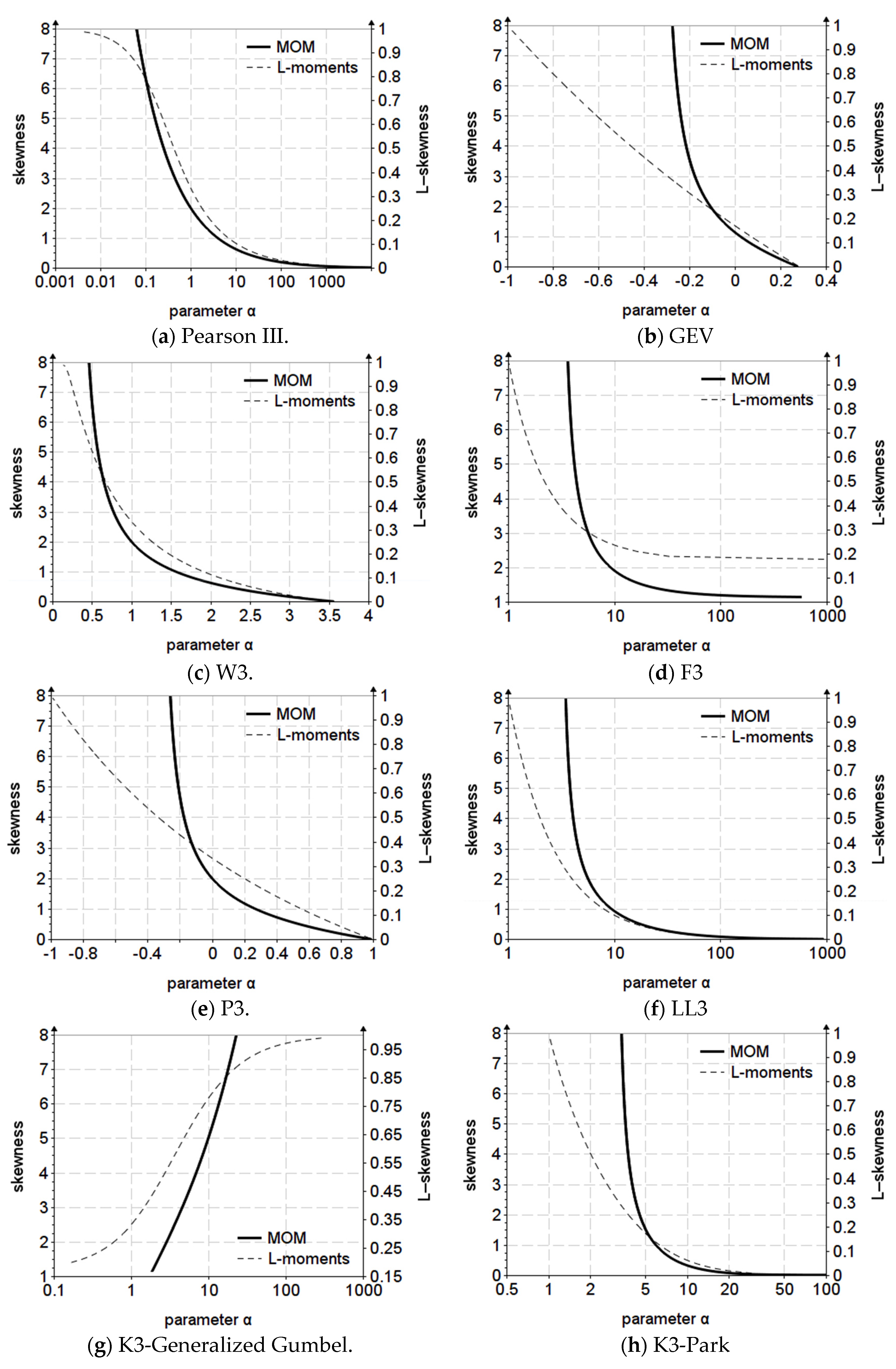
The variation graph of skewness (${\mathrm{C}}_{\mathrm{s}}$) for the first vertical axis and L-skewness (${\mathrm{\tau }}_3$) and for the vertical secondary axis, depending on the parameter $\mathsf{\alpha }$ are presented in Figure 1.

Figure 1. The variation of parameter α for three parameters distributions.

For two-parameter distributions, the definition range of the $\mathsf{\alpha }$ variable was determined as a function of ${\mathrm{C}}_{\mathrm{v}}$ for MOM and ${\mathrm{\tau }}_2$ for L-moments. The limits of the definition domain of the parameter $\mathsf{\alpha }$ were established according to the extreme values of ${\mathrm{C}}_{\mathrm{v}}$ and ${\mathrm{\tau }}_2$, thus ${\mathrm{\tau }}_2$ was calculated for $0<{\mathrm{C}}_{\mathrm{v}}\le 2$, respectively, for $0<{\mathrm{\tau }}_2<1$. The functions ${\mathrm{C}}_{\mathrm{v}}\left(\mathsf{\alpha }\right)$ and ${\mathrm{\tau }}_2\left(\mathsf{\alpha }\right)$ were plotted for both methods.

The variation graph of coefficient of variation for the first vertical axis (${\mathrm{C}}_{\mathrm{v}}$) and L-coefficient of variation (${\mathrm{\tau }}_2$) for the vertical secondary axis, depending on the parameter $\mathsf{\alpha }$ are presented in Figure 2.

Figure 2. The variation of parameter α for two parameters distributions.

Graphical examination indicated the type of approximation functions. The first-order derivatives were calculated to determine the slope variation, so for uniform variations over certain intervals a type of function is defined. If the variation is uniform in logarithmic scale, then the argument of the function is chosen logarithmically for the approximation with a polynomial, otherwise the rational function is chosen without logarithmization. The rational function is the ratio of two polynomial functions. There were situations in which the rational function was reduced only to a polynomial function, because “the denominator” represents a constant equal to one. For some probability distributions, the same type of functions, rational or polynomial, were used, and in some cases both functions were used on some distinct defining intervals.

The attempts that were made for approximation functions took into account existing approximations for some distributions [6,11]. The approximation functions considered optimal in terms of relative errors and number of terms were chosen, ensuring a balance between the relative error allowed and the complexity of the relationship.

The calibration of the approximation functions was carried out with the linear least squares method for the polynomial functions and nonlinear for the rational functions.

3.2. Methods of Parameter Estimation

In this article, two methods of parameters estimation are studied: the method of ordinary moments (MOM) and the L-moments method.

3.2.1. Pearson III Distribution (PE3)

For estimation with MOM, the distribution parameters have the following expressions [10]:

$$\mathsf{\alpha }={\left(\frac{2}{{\mathrm{C}}_{\mathrm{s}}}\right)}^2$$

(42)

$$\mathsf{\beta }=\frac{\mathrm{\sigma }}{2}·{\mathrm{C}}_{\mathrm{s}}$$

(43)

$$\mathrm{\gamma }=\mathsf{\mu }-\mathsf{\alpha }·\mathsf{\beta }$$

(44)

where ${\mathrm{C}}_{\mathrm{s}}$ represents the skewness coefficient.

The parameter $\mathsf{\alpha }$ can be estimated using the rational function presented by Hosking in 1997, named in this section the “Hosking approximation”, or based on an approximation made up of two polynomial functions and one rational, depending on the definition domain of the estimated parameter, named here “a better approximation”.

Thus, for the estimation with the L-moments, the shape parameter $\mathsf{\alpha }$ can be evaluated numerically with the following approximate forms, depending on L-skewness (${\mathrm{\tau }}_3$):

The Hosking approximation, rational function [11,14]:

If $0<\left|{\mathrm{\tau }}_3\right|<\frac{1}{3}$:

$$\mathsf{\alpha }=\frac{1+2.73884·{\mathrm{\tau }}_3^2}{9.424778·{\mathrm{\tau }}_3^2+16.7171359·{\mathrm{\tau }}_3^4+37.0028906·{\mathrm{\tau }}_3^6}$$

(45)

if $\frac{1}{3}\le \left|{\mathrm{\tau }}_3\right|<1$:

$$\mathsf{\alpha }=\frac{0.36067·\left(1-\left|{\mathrm{\tau }}_3\right|\right)-0.59567·{\left(1-\left|{\mathrm{\tau }}_3\right|\right)}^2+0.25361·{\left(1-\left|{\mathrm{\tau }}_3\right|\right)}^3}{1-2.78861·\left(1-\left|{\mathrm{\tau }}_3\right|\right)+2.56096·{\left(1-\left|{\mathrm{\tau }}_3\right|\right)}^2-0.77045·{\left(1-\left|{\mathrm{\tau }}_3\right|\right)}^3}$$

(46)

better approximation, polynomial and rational functions:

If $0<\left|{\mathrm{\tau }}_3\right|\le \frac{1}{3}$:

$$\mathsf{\alpha }=\exp \left(\begin{array}{l}-3.164791927-5.108735285·\ln \left(\left|{\mathrm{\tau }}_3\right|\right)-4.116014079·\ln {\left(\left|{\mathrm{\tau }}_3\right|\right)}^2-\\ 2.985250105·\ln {\left(\left|{\mathrm{\tau }}_3\right|\right)}^3-1.327399577·\ln {\left(\left|{\mathrm{\tau }}_3\right|\right)}^4-0.373944875·\ln {\left(\left|{\mathrm{\tau }}_3\right|\right)}^5-\\ 0.065421611·\ln {\left(\left|{\mathrm{\tau }}_3\right|\right)}^6-0.006508037·\ln {\left(\left|{\mathrm{\tau }}_3\right|\right)}^7-0.000281969·\ln {\left(\left|{\mathrm{\tau }}_3\right|\right)}^8\end{array}\right)$$

(47)

if $\frac{1}{3}<\left|{\mathrm{\tau }}_3\right|\le \frac{2}{3}$:

$$\mathsf{\alpha }=\exp \left(\begin{array}{l}-3.9918551-10.781466·\ln \left(\left|{\mathrm{\tau }}_3\right|\right)-21.557807·\ln {\left(\left|{\mathrm{\tau }}_3\right|\right)}^2-\\ 33.8752604·\ln {\left(\left|{\mathrm{\tau }}_3\right|\right)}^3-35.0641585·\ln {\left(\left|{\mathrm{\tau }}_3\right|\right)}^4-22.921163·\ln {\left(\left|{\mathrm{\tau }}_3\right|\right)}^5-\\ 8.5491823·\ln {\left(\left|{\mathrm{\tau }}_3\right|\right)}^6-1.3855653·\ln {\left(\left|{\mathrm{\tau }}_3\right|\right)}^7\end{array}\right)$$

(48)

if $\frac{2}{3}<\left|{\mathrm{\tau }}_3\right|<1$:

$$\mathsf{\alpha }=\frac{\begin{array}{l}5.17817436-26.209448756·\left|{\mathrm{\tau }}_3\right|+62.12494027·{\mathrm{\tau }}_3^2-84.39423264·{\left|{\mathrm{\tau }}_3\right|}^3+\\ 67.08589624·{\mathrm{\tau }}_3^4-29.150288079·{\left|{\mathrm{\tau }}_3\right|}^5+5.364968945·{\mathrm{\tau }}_3^6\end{array}}{1+0.0005134·\left|{\mathrm{\tau }}_3\right|+0.00063644·{\mathrm{\tau }}_3^2}$$

(49)

The scale parameter $\mathsf{\beta }$ and the position parameter $\mathrm{\gamma }$ are determined with the following expressions [14]:

$$\mathsf{\beta }={\mathrm{L}}_2·\sqrt{\mathrm{\pi }}·\frac{\mathrm{\Gamma }\left(\mathsf{\alpha }\right)}{\mathrm{\Gamma }\left(\mathsf{\alpha }+\frac{1}{2}\right)}$$

(50)

$$\mathrm{\gamma }={\mathrm{L}}_1-\mathsf{\alpha }·\mathsf{\beta }$$

(51)

where ${\mathrm{L}}_1,{\mathrm{L}}_2,{\mathrm{\tau }}_3$ are the sample L-moments and L-skewness, [7,11,14].

3.2.2. Generalized Extreme Value Distribution (GEV)

The parameter $\mathsf{\alpha }$ can be estimated using the “approximation 1”, which represents a polynomial function presented by Rao et.al [11], or using two new approximations of the polynomial or rational type, hereafter named “approximation 2” and “approximation 3”.

Thus, the parameter $\mathsf{\alpha }$ has the following approximate forms depending on ${\mathrm{C}}_{\mathrm{s}}$:

Approximation 1, polynomial function [11]:

If ${\mathrm{C}}_{\mathrm{s}}\le 1.14$:

$$\begin{array}{l}\mathsf{\alpha }=0.277648-0.322016·{\mathrm{C}}_{\mathrm{s}}+0.060278·{\mathrm{C}}_{\mathrm{s}}^2+0.016759·{\mathrm{C}}_{\mathrm{s}}^3-\\ 0.005873·{\mathrm{C}}_{\mathrm{s}}^4-0.00244·{\mathrm{C}}_{\mathrm{s}}^5-0.000050·{\mathrm{C}}_{\mathrm{s}}^6\end{array}$$

(52)

if ${\mathrm{C}}_{\mathrm{s}}>1.14$:

$$\begin{array}{l}\mathsf{\alpha }=0.2858221-0.357983·{\mathrm{C}}_{\mathrm{s}}+0.116659·{\mathrm{C}}_{\mathrm{s}}^2-0.022725·{\mathrm{C}}_{\mathrm{s}}^3+\\ 0.002604·{\mathrm{C}}_{\mathrm{s}}^4-0.000161·{\mathrm{C}}_{\mathrm{s}}^5+0.000004·{\mathrm{C}}_{\mathrm{s}}^6\end{array}$$

(53)

better approximations:

Approximation 2, polynomial form:

If ${\mathrm{C}}_{\mathrm{s}}\le 1.14$:

$$\begin{array}{l}\mathsf{\alpha }=0.2775961-0.3217629·{\mathrm{C}}_{\mathrm{s}}+0.0608352·{\mathrm{C}}_{\mathrm{s}}^2+0.0170626·{\mathrm{C}}_{\mathrm{s}}^3-\\ 0.0100647·{\mathrm{C}}_{\mathrm{s}}^4+0.0004883·{\mathrm{C}}_{\mathrm{s}}^5+0.0003895·{\mathrm{C}}_{\mathrm{s}}^6\end{array}$$

(54)

If ${\mathrm{C}}_{\mathrm{s}}>1.14$:

$$\begin{array}{l}\mathrm{\alpha }=0.2786297-0.3425507\cdot {\mathrm{C}}_{\mathrm{s}}+0.1041188\cdot {\mathrm{C}}_{\mathrm{s}}^2-0.0177578\cdot {\mathrm{C}}_{\mathrm{s}}^3\\ +0.001584\cdot {\mathrm{C}}_{\mathrm{s}}^4-0.0000572\cdot {\mathrm{C}}_{\mathrm{s}}^5\end{array}$$

(55)

Approximation 3, rational form:

$$\mathsf{\alpha }=\frac{0.277593723-0.116805709·{\mathrm{C}}_{\mathrm{s}}-0.071360121·{\mathrm{C}}_{\mathrm{s}}^2-0.035014727·{\mathrm{C}}_{\mathrm{s}}^3}{1+0.73874734·{\mathrm{C}}_{\mathrm{s}}+0.37485038·{\mathrm{C}}_{\mathrm{s}}^2+0.103516119·{\mathrm{C}}_{\mathrm{s}}^3}$$

(56)

$$\mathsf{\beta }=\frac{\mathsf{\alpha }}{\left|\mathsf{\alpha }\right|}\cdot \frac{\mathrm{\sigma }\cdot \mathsf{\alpha }}{\sqrt{\mathrm{\Gamma }\left(1+2\cdot \mathsf{\alpha }\right)-\mathrm{\Gamma }{\left(1+\mathsf{\alpha }\right)}^2}}$$

(57)

$$\mathrm{\gamma }=\mathsf{\mu }-\frac{\mathsf{\alpha }}{\left|\mathsf{\alpha }\right|}·\frac{\mathrm{\sigma }·\left[1-\mathrm{\Gamma }\left(1+\mathsf{\alpha }\right)\right]}{\sqrt{\mathrm{\Gamma }\left(1+2·\mathsf{\alpha }\right)-\mathrm{\Gamma }{\left(1+\mathsf{\alpha }\right)}^2}}$$

(58)

For estimation with the L-moments, parameter $\mathsf{\alpha }$ has the following approximate forms depending on ${\mathrm{\tau }}_3$:

Approximation 1, polynomial form, presented in Rao et al. [11] and Hosking [14]:

$$\mathsf{\alpha }=7.85890·\left(\frac{2}{3+{\mathrm{\tau }}_3}-\frac{\ln \left(2\right)}{\ln \left(3\right)}\right)+2.9554·{\left(\frac{2}{3+{\mathrm{\tau }}_3}-\frac{\ln \left(2\right)}{\ln \left(3\right)}\right)}^2$$

(59)

Approximation 2, also a polynomial function but more accurate, presented in Rao et al. [11]:

$$\begin{array}{l}\mathsf{\alpha }=7.817740·\left(\frac{2}{3+{\mathrm{\tau }}_3}-\frac{\ln \left(2\right)}{\ln \left(3\right)}\right)+2.930462·{\left(\frac{2}{3+{\mathrm{\tau }}_3}-\frac{\ln \left(2\right)}{\ln \left(3\right)}\right)}^2+\\ 13.641492·{\left(\frac{2}{3+{\mathrm{\tau }}_3}-\frac{\ln \left(2\right)}{\ln \left(3\right)}\right)}^3+17.206675·{\left(\frac{2}{3+{\mathrm{\tau }}_3}-\frac{\ln \left(2\right)}{\ln \left(3\right)}\right)}^4\end{array}$$

(60)

a better approximation, named in this section approximation 3, being a rational function:

$$\mathsf{\alpha }=\frac{0.283759107-1.669931462·\left|{\mathrm{\tau }}_3\right|}{1+0.441588375·\left|{\mathrm{\tau }}_3\right|-0.071007671·{\mathrm{\tau }}_3^2+0.015634368·{\left|{\mathrm{\tau }}_3\right|}^3}$$

(61)

$$\mathsf{\beta }=\frac{{\mathrm{L}}_2}{\mathrm{\Gamma }\left(\mathsf{\alpha }\right)·\left(1-2^{-\mathsf{\alpha }}\right)}$$

(62)

$$\mathrm{\gamma }={\mathrm{L}}_1+\frac{\mathsf{\beta }}{\mathsf{\alpha }}·\left[\mathrm{\Gamma }\left(1+\mathsf{\alpha }\right)-1\right]$$

(63)

3.2.3. Weibull Distribution (W3)

For estimation with MOM, parameter $\mathsf{\alpha }$ can be approximated, depending on the skewness, using the “approximation 1” of the rational function type presented by Rao, valid for a maximum skewness of 2, or using the new approximation called here “a better approximation” valid for a skewness in the range of 0–8:

Approximation 1, for ${\mathrm{C}}_{\mathrm{s}}\le 2$, [11]:

$$\mathsf{\alpha }=\frac{1}{\begin{array}{l}0.2777561+0.3219·{\mathrm{C}}_{\mathrm{s}}+0.061566·{\mathrm{C}}_{\mathrm{s}}^2-0.017376·{\mathrm{C}}_{\mathrm{s}}^3-\\ 0.00771·{\mathrm{C}}_{\mathrm{s}}^4+0.00398·{\mathrm{C}}_{\mathrm{s}}^5-0.00051·{\mathrm{C}}_{\mathrm{s}}^6\end{array}}$$

(64)

a better approximation, called here approximation 2, valid for $0<{\mathrm{C}}_{\mathrm{s}}\le 8$:

$$\mathsf{\alpha }=\frac{\begin{array}{l}3.5947875-3.7374529·{\mathrm{C}}_{\mathrm{s}}+2.7023151·{\mathrm{C}}_{\mathrm{s}}^2-1.1835102·{\mathrm{C}}_{\mathrm{s}}^3+\\ 0.4318107·{\mathrm{C}}_{\mathrm{s}}^4-0.0042306·{\mathrm{C}}_{\mathrm{s}}^5+0.0045545·{\mathrm{C}}_{\mathrm{s}}^6-0.0046984·{\mathrm{C}}_{\mathrm{s}}^7\end{array}}{\begin{array}{l}1+0.0931316·{\mathrm{C}}_{\mathrm{s}}-0.12783·{\mathrm{C}}_{\mathrm{s}}^2+0.0671082·{\mathrm{C}}_{\mathrm{s}}^3+0.1113667·{\mathrm{C}}_{\mathrm{s}}^4-\\ 0.0425475·{\mathrm{C}}_{\mathrm{s}}^5+0.0673629·{\mathrm{C}}_{\mathrm{s}}^6-0.0157628·{\mathrm{C}}_{\mathrm{s}}^7\end{array}}$$

(65)

$$\mathsf{\beta }=\frac{\mathrm{\sigma }}{\sqrt{\mathrm{\Gamma }\left(1+\frac{2}{\mathsf{\alpha }}\right)-\mathrm{\Gamma }{\left(1+\frac{1}{\mathsf{\alpha }}\right)}^2}}$$

(66)

$$\mathrm{\gamma }=\mathsf{\mu }-\mathsf{\beta }·\mathrm{\Gamma }\left(1+\frac{1}{\mathsf{\alpha }}\right)$$

(67)

For estimation with the L-moments, parameter $\mathsf{\alpha }$ has the following approximate forms depending on ${\mathrm{\tau }}_3$:

Approximation 1, a rational function presented by Rao et al. [11]:

$$\mathsf{\alpha }=\frac{1}{7.85890·\left(\frac{2}{3-{\mathrm{\tau }}_3}-\frac{\log \left(2\right)}{\log \left(3\right)}\right)+2.9554·{\left(\frac{2}{3-{\mathrm{\tau }}_3}-\frac{\log \left(2\right)}{\log \left(3\right)}\right)}^2}$$

(68)

Approximation 2, polynomial form, for positive ${\mathrm{\tau }}_3$, presented by Y.Goda [15]:

$$\mathsf{\alpha }=285.3·{\mathrm{\tau }}_3^6-658.6·{\mathrm{\tau }}_3^5+622.8·{\mathrm{\tau }}_3^4-317.2·{\mathrm{\tau }}_3^3+98.52·{\mathrm{\tau }}_3^2-21.256·{\mathrm{\tau }}_3+3.516$$

(69)

a better approximation, named here approximation 3, which is a rational function, valid for negative and positive values of L-skewness:

$$\mathsf{\alpha }=\frac{3.528107902-6.294082546·\left|{\mathrm{\tau }}_3\right|+2.767652838·{\mathrm{\tau }}_3^2}{1+4.599024923·\left|{\mathrm{\tau }}_3\right|-7.993601572·{\mathrm{\tau }}_3^2+2.423742593·{\left|{\mathrm{\tau }}_3\right|}^3}$$

(70)

$$\mathsf{\beta }=\frac{{\mathrm{L}}_2}{\mathrm{\Gamma }\left(1+\frac{1}{\mathsf{\alpha }}\right)·\left(1-2^{-\frac{1}{\mathsf{\alpha }}}\right)}$$

(71)

$$\mathrm{\gamma }={\mathrm{L}}_1-\frac{\mathsf{\beta }}{\mathsf{\alpha }}·\mathrm{\Gamma }\left(\frac{1}{\mathsf{\alpha }}\right)$$

(72)

3.2.4. Weibull Distribution (W2)

For estimation with MOM, parameter $\mathsf{\alpha }$ has the following approximate forms depending on the coefficient of variation ${\mathrm{C}}_{\mathrm{v}}\ge 0.1$:

$$\mathsf{\alpha }=\exp \left(\begin{array}{l}0.000006199-1.000228322·\ln \left({\mathrm{C}}_{\mathrm{v}}\right)+0.144564211·\ln {\left({\mathrm{C}}_{\mathrm{v}}\right)}^2+\\ 0.055543308·\ln {\left({\mathrm{C}}_{\mathrm{v}}\right)}^3-0.016265526·\ln {\left({\mathrm{C}}_{\mathrm{v}}\right)}^4-0.013691787·\ln {\left({\mathrm{C}}_{\mathrm{v}}\right)}^5-\\ 0.000586501·\ln {\left({\mathrm{C}}_{\mathrm{v}}\right)}^6+0.001239068·\ln {\left({\mathrm{C}}_{\mathrm{v}}\right)}^7+0.000240162·\ln {\left({\mathrm{C}}_{\mathrm{v}}\right)}^8\end{array}\right)$$

(73)

$$\mathsf{\beta }=\frac{\mathsf{\mu }}{\mathrm{\Gamma }\left(1+\frac{1}{\mathsf{\alpha }}\right)}$$

(74)

For estimation with the L-moments, parameters have the following expressions [11,16,17]:

$$\mathsf{\alpha }=\frac{-\ln \left(2\right)}{\ln \left(1-\frac{{\mathrm{L}}_2}{{\mathrm{L}}_1}\right)}$$

(75)

$$\mathsf{\beta }=\frac{{\mathrm{L}}_1}{\mathrm{\Gamma }\left(1+\frac{1}{\mathsf{\alpha }}\right)}$$

(76)

3.2.5. Fréchet Distribution (F3)

For estimation with MOM, parameter $\mathsf{\alpha }$ has the following approximate forms depending on ${\mathrm{C}}_{\mathrm{s}}$:

Rational approximation form, for ${\mathrm{C}}_{\mathrm{s}}>1.14$:

$$\mathsf{\alpha }=\frac{1+0.73874734·{\mathrm{C}}_{\mathrm{s}}+0.37485038·{\mathrm{C}}_{\mathrm{s}}^2+0.103516119·{\mathrm{C}}_{\mathrm{s}}^3}{-0.277593723+0.116805709·{\mathrm{C}}_{\mathrm{s}}+0.071360121·{\mathrm{C}}_{\mathrm{s}}^2+0.035014727·{\mathrm{C}}_{\mathrm{s}}^3}$$

(77)

$$\mathsf{\beta }=\frac{\mathrm{\sigma }}{\sqrt{\mathrm{\Gamma }\left(1-\frac{2}{\mathsf{\alpha }}\right)-\mathrm{\Gamma }{\left(1-\frac{1}{\mathsf{\alpha }}\right)}^2}}$$

(78)

$$\mathrm{\gamma }=\mathsf{\mu }-\mathsf{\beta }·\mathrm{\Gamma }\left(1-\frac{1}{\mathsf{\alpha }}\right)$$

(79)

For estimation with the L-moments, parameter $\mathsf{\alpha }$ has the following approximate forms depending on L-skewness, $\left|{\mathrm{\tau }}_3\right|\ge 0.17$:

Approximation 1, a rational function, adopted from GEV approximation [11]:

$$\mathsf{\alpha }=\frac{1}{\left(\begin{array}{l}-7.817740·\left(\frac{2}{3+{\mathrm{\tau }}_3}-\frac{\ln \left(2\right)}{\ln \left(3\right)}\right)-2.930462·{\left(\frac{2}{3+{\mathrm{\tau }}_3}-\frac{\ln \left(2\right)}{\ln \left(3\right)}\right)}^2-\\ 13.641492·{\left(\frac{2}{3+{\mathrm{\tau }}_3}-\frac{\ln \left(2\right)}{\ln \left(3\right)}\right)}^3-17.206675·{\left(\frac{2}{3+{\mathrm{\tau }}_3}-\frac{\ln \left(2\right)}{\ln \left(3\right)}\right)}^4\end{array}\right)}$$

(80)

a better approximation, named here approximation 2, also a rational function form but characterized by smaller relative errors in the range of 0.6–1 of the L-skewness:

$$\mathsf{\alpha }=\frac{1+0.441588375·\left|{\mathrm{\tau }}_3\right|-0.071007671·{\mathrm{\tau }}_3^2+0.015634368·{\left|{\mathrm{\tau }}_3\right|}^3}{-0.283759107+1.669931462·\left|{\mathrm{\tau }}_3\right|}$$

(81)

$$\mathsf{\beta }=\frac{{\mathrm{L}}_2}{\mathrm{\Gamma }\left(-\frac{1}{\mathsf{\alpha }}\right)·\left(1-2^{-\frac{1}{\mathsf{\alpha }}}\right)}$$

(82)

$$\mathrm{\gamma }={\mathrm{L}}_1-\mathsf{\beta }·\mathrm{\Gamma }\left(1-\frac{1}{\mathsf{\alpha }}\right)$$

(83)

3.2.6. Fréchet Distribution (F2)

For estimation with MOM, parameter $\mathsf{\alpha }$ has the following approximate forms depending on the coefficient of variation ${\mathrm{C}}_{\mathrm{v}}$:

$$\mathsf{\alpha }=\exp \left(\begin{array}{l}0.928192087-0.358563901·\ln \left({\mathrm{C}}_{\mathrm{v}}\right)+0.206039026·\ln {\left({\mathrm{C}}_{\mathrm{v}}\right)}^2-\\ 0.023717668·\ln {\left({\mathrm{C}}_{\mathrm{v}}\right)}^3-0.029286344·\ln {\left({\mathrm{C}}_{\mathrm{v}}\right)}^4+0.003741887·\ln {\left({\mathrm{C}}_{\mathrm{v}}\right)}^5+\\ 0.008353766·\ln {\left({\mathrm{C}}_{\mathrm{v}}\right)}^6+0.002758305·\ln {\left({\mathrm{C}}_{\mathrm{v}}\right)}^7+0.000306859·\ln {\left({\mathrm{C}}_{\mathrm{v}}\right)}^8\end{array}\right)$$

(84)

$$\mathsf{\beta }=\frac{\mathsf{\mu }}{\mathrm{\Gamma }\left(1-\frac{1}{\mathsf{\alpha }}\right)}$$

(85)

For estimation with the L-moments, parameters have the following expressions [15]:

$$\mathsf{\alpha }=\frac{\ln \left(2\right)}{\ln \left(\frac{{\mathrm{L}}_2+{\mathrm{L}}_1}{{\mathrm{L}}_1}\right)}$$

(86)

$$\mathsf{\beta }=\frac{{\mathrm{L}}_1}{\mathrm{\Gamma }\left(1-\frac{1}{\mathsf{\alpha }}\right)}$$

(87)

3.2.7. Generalized Pareto Distribution (P3)

For estimation with MOM, parameter $\mathsf{\alpha }$ has the following approximate polynomial or rational forms depending on ${\mathrm{C}}_{\mathrm{s}}$:

For ${\mathrm{C}}_{\mathrm{s}}\le 2$:

$$\begin{array}{l}\mathsf{\alpha }=999.998156889·{10}^{-3}-1.154659839·{\mathrm{C}}_{\mathrm{s}}+555.214061169·{10}^{-3}·{\mathrm{C}}_{\mathrm{s}}^2-\\ 137.553895649·{10}^{-3}·{\mathrm{C}}_{\mathrm{s}}^3-2.365065448·{10}^{-3}·{\mathrm{C}}_{\mathrm{s}}^4+13.308919064·{10}^{-3}·{\mathrm{C}}_{\mathrm{s}}^5-\\ 3.931108819·{10}^{-3}·{\mathrm{C}}_{\mathrm{s}}^6+409.717304137·{10}^{-6}·{\mathrm{C}}_{\mathrm{s}}^7\end{array}$$

(88)

for ${\mathrm{C}}_{\mathrm{s}}>2$:

$$\mathsf{\alpha }=\frac{\begin{array}{l}880.965365848·{10}^{-3}-926.199345052·{10}^{-3}·{\mathrm{C}}_{\mathrm{s}}+394.547875439·{10}^{-3}·{\mathrm{C}}_{\mathrm{s}}^2-\\ 103.261733369·{10}^{-3}·{\mathrm{C}}_{\mathrm{s}}^3+16.938774757·{10}^{-3}·{\mathrm{C}}_{\mathrm{s}}^4-1.812785982·{10}^{-3}·{\mathrm{C}}_{\mathrm{s}}^5+\\ 103.169053863·{10}^{-6}·{\mathrm{C}}_{\mathrm{s}}^6-2.562841773·{10}^{-6}·{\mathrm{C}}_{\mathrm{s}}^7\end{array}}{\begin{array}{l}1+449.853791343·{10}^{-6}·{\mathrm{C}}_{\mathrm{s}}+1.18940502·{10}^{-3}·{\mathrm{C}}_{\mathrm{s}}^2+\\ 353.672107629·{10}^{-6}·{\mathrm{C}}_{\mathrm{s}}^3+1.35505086·{10}^{-3}·{\mathrm{C}}_{\mathrm{s}}^4+84.527491397·{10}^{-6}·{\mathrm{C}}_{\mathrm{s}}^5\end{array}}$$

(89)

$$\mathsf{\beta }=\mathrm{\sigma }·\left(\mathsf{\alpha }+1\right)·\sqrt{2·\mathsf{\alpha }+1}$$

(90)

$$\mathrm{\gamma }=\mathsf{\mu }-\frac{\mathsf{\beta }}{\mathsf{\alpha }+1}$$

(91)

For estimation with the L-moments, parameters have the following expressions [11,14,16,17]:

$$\mathsf{\alpha }=\frac{1-3·{\mathrm{\tau }}_3}{{\mathrm{\tau }}_3+1}$$

(92)

$$\mathsf{\beta }={\mathrm{L}}_2·\left(1+\mathsf{\alpha }\right)·\left(2+\mathsf{\alpha }\right)$$

(93)

$$\mathrm{\gamma }={\mathrm{L}}_1-{\mathrm{L}}_2·\left(2+\mathsf{\alpha }\right)$$

(94)

3.2.8. Log-Logistic Distribution (LL3)

For estimation with MOM, parameter $\mathsf{\alpha }$ has the following approximate forms depending on ${\mathrm{C}}_{\mathrm{s}}>0$:

Approximation 1, adopted from the expression for generalized Logistic [11,19]:

For ${\mathrm{C}}_{\mathrm{s}}\le 2.5$, the approximation function is polynomial:

$$\mathsf{\alpha }=\exp \left(2.246-0.848·\ln \left({\mathrm{C}}_{\mathrm{s}}\right)+0.1272·\ln {\left({\mathrm{C}}_{\mathrm{s}}\right)}^2-0.04008·\ln {\left({\mathrm{C}}_{\mathrm{s}}\right)}^3\right)$$

(95)

for ${\mathrm{C}}_{\mathrm{s}}>2.5$, the approximation function has a rational form:

$$\mathsf{\alpha }=\frac{4.007+3.411·{\mathrm{C}}_{\mathrm{s}}+2.985·{\mathrm{C}}_{\mathrm{s}}^2}{{\mathrm{C}}_{\mathrm{s}}^2}$$

(96)

approximation 2, adopted from the expression for generalized Logistic [11]:

$$\mathsf{\alpha }=\frac{-3·\mathrm{\pi }}{2·\mathrm{a}\tan \left(-0.59484·{\mathrm{C}}_{\mathrm{s}}\right)}$$

(97)

a better approximation referred here as approximation 3, which is a polynomial function:

For ${\mathrm{C}}_{\mathrm{s}}\le 2.5$:

$$\mathsf{\alpha }=\exp \left(\begin{array}{l}2.22464301-850.7876728·{10}^{-3}·\ln \left({\mathrm{C}}_{\mathrm{s}}\right)+121.776022·{10}^{-3}·\ln {\left({\mathrm{C}}_{\mathrm{s}}\right)}^2+\\ 51.4528279·{10}^{-3}·\ln {\left({\mathrm{C}}_{\mathrm{s}}\right)}^3+5.3737403·{10}^{-3}·\ln {\left({\mathrm{C}}_{\mathrm{s}}\right)}^4-\\ 2.8910802·{10}^{-3}·\ln {\left({\mathrm{C}}_{\mathrm{s}}\right)}^5-3.2030341·{10}^{-3}·\ln {\left({\mathrm{C}}_{\mathrm{s}}\right)}^6-\\ 671.4922523·{10}^{-6}·\ln {\left({\mathrm{C}}_{\mathrm{s}}\right)}^7-51.670024·{10}^{-6}·\ln {\left({\mathrm{C}}_{\mathrm{s}}\right)}^8\end{array}\right)$$

(98)

for ${\mathrm{C}}_{\mathrm{s}}>2.5$:

$$\begin{array}{l}\mathsf{\alpha }=15.786327481-11.37147504·{\mathrm{C}}_{\mathrm{s}}+5.201363981·{\mathrm{C}}_{\mathrm{s}}^2-\\ 1.418144703·{\mathrm{C}}_{\mathrm{s}}^3+0.239556022·{\mathrm{C}}_{\mathrm{s}}^4-0.02462292·{\mathrm{C}}_{\mathrm{s}}^5+\\ 0.001412092·{\mathrm{C}}_{\mathrm{s}}^6-0.00003466·{\mathrm{C}}_{\mathrm{s}}^7\end{array}$$

(99)

$$\mathsf{\beta }=\frac{\mathrm{\sigma }}{\sqrt{\mathrm{\Gamma }\left(1+\frac{2}{\mathsf{\alpha }}\right)·\mathrm{\Gamma }\left(1-\frac{2}{\mathsf{\alpha }}\right)-\mathrm{\Gamma }{\left(1+\frac{1}{\mathsf{\alpha }}\right)}^2·\mathrm{\Gamma }{\left(1-\frac{1}{\mathsf{\alpha }}\right)}^2}}$$

(100)

$$\mathrm{\gamma }=\mathsf{\mu }-\frac{\mathsf{\beta }}{\mathsf{\alpha }}·\mathrm{\Gamma }\left(\frac{1}{\mathsf{\alpha }}\right)·\mathrm{\Gamma }\left(1-\frac{1}{\mathsf{\alpha }}\right)$$

(101)

For estimation with L-moments, parameters have the following expressions [11]:

$$\mathsf{\alpha }=\frac{{\mathrm{L}}_2}{{\mathrm{L}}_3}$$

(102)

$$\mathsf{\beta }=\frac{{\mathsf{\alpha }}^2·{\mathrm{L}}_2}{\mathrm{\Gamma }\left(\frac{1}{\mathsf{\alpha }}\right)·\mathrm{\Gamma }\left(1-\frac{1}{\mathsf{\alpha }}\right)}$$

(103)

$$\mathrm{\gamma }={\mathrm{L}}_1-\frac{\mathsf{\beta }}{\mathsf{\alpha }}·\mathrm{\Gamma }\left(\frac{1}{\mathsf{\alpha }}\right)·\mathrm{\Gamma }\left(1-\frac{1}{\mathsf{\alpha }}\right)$$

(104)

3.2.9. Kappa Distribution (K3-Generalized Gumbel)

For estimation with MOM, parameter $\mathsf{\alpha }$ has the following approximate polynomial form, for ${\mathrm{C}}_{\mathrm{s}}>1.14$:

$$\begin{array}{l}\mathsf{\alpha }=-918.79032552·{10}^{-3}+768.82077754·{10}^{-3}·{\mathrm{C}}_{\mathrm{s}}-91.79270267·{10}^{-3}·{\mathrm{C}}_{\mathrm{s}}^2+\\ 136.3152042·{10}^{-3}·{\mathrm{C}}_{\mathrm{s}}^3-27.00071596·{10}^{-3}·{\mathrm{C}}_{\mathrm{s}}^4+3.20994481·{10}^{-3}·{\mathrm{C}}_{\mathrm{s}}^5-\\ 210.04317387·{10}^{-6}·{\mathrm{C}}_{\mathrm{s}}^6+5.80948381·{10}^{-6}·{\mathrm{C}}_{\mathrm{s}}^7\end{array}$$

(105)

$$\mathsf{\beta }=\frac{\mathrm{\sigma }}{{\left(\frac{\begin{array}{l}7.7175·{\mathsf{\alpha }}^8-326.34·{\mathsf{\alpha }}^7-3711.7·{\mathsf{\alpha }}^6+\\ 67724.37·{\mathsf{\alpha }}^5+321482.3241·{\mathsf{\alpha }}^4-\\ 7529351.76·{\mathsf{\alpha }}^3+38043509.47·{\mathsf{\alpha }}^2-\\ 19935867.29·\mathsf{\alpha }+219479848.41\end{array}}{115221657.6}{\left(\mathrm{\psi }\left(\frac{1}{\mathsf{\alpha }}+1\right)+\ln \left(\mathsf{\alpha }\right)+{\mathrm{\gamma }}_{\mathrm{e}}\right)}^2\right)}^{0.5}}$$

(106)

$$\mathrm{\gamma }=\mathsf{\mu }-\mathsf{\beta }·\left(\mathsf{\psi }\left(\frac{1}{\mathsf{\alpha }}+1\right)+\ln \left(\mathsf{\alpha }\right)+{\mathrm{\gamma }}_{\mathrm{e}}\right)$$

(107)

where ${\mathrm{\gamma }}_{\mathrm{e}}$ is the Euler–Mascheroni constant and $\mathsf{\psi }\left(..\right)$ represents the digamma function, which has the following approximate form [11]:

$$\begin{array}{l}\mathsf{\psi }\left(\mathsf{\alpha }\right)=\frac{\mathrm{d}}{\mathrm{d}\mathsf{\alpha }}\left(\ln \left(\mathrm{\Gamma }\left(\mathsf{\alpha }\right)\right)\right)=\mathrm{P}\mathrm{s}\mathrm{i}\left(\mathsf{\alpha }\right)\\ \mathsf{\psi }\left(\mathsf{\alpha }\right)\approx \mathrm{l}\mathrm{n}\left(\mathsf{\alpha }+2\right)-\frac{1}{\mathsf{\alpha }}-\frac{1}{\mathsf{\alpha }+1}-\frac{1}{2·\left(\mathsf{\alpha }+2\right)}-\frac{1}{12·{\left(\mathsf{\alpha }+2\right)}^2}+\frac{1}{120·{\left(\mathsf{\alpha }+2\right)}^4}\end{array}$$

(108)

For estimation with the L-moments, parameter $\mathsf{\alpha }$ has the following approximate forms depending on ${\mathrm{\tau }}_3$:

For $0.17\le \left|{\mathrm{\tau }}_3\right|\le \frac{1}{3}$:

$$\mathsf{\alpha }=-971.10886182·{10}^{-3}+6.3606944·\left|{\mathrm{\tau }}_3\right|-6.35405524·{\mathrm{\tau }}_3^2+15.03572719·{\left|{\mathrm{\tau }}_3\right|}^3$$

(109)

for $\frac{1}{3}<\left|{\mathrm{\tau }}_3\right|<1$:

$$\mathsf{\alpha }=\frac{-661.76303922·{10}^{-3}+4.30832382·\left|{\mathrm{\tau }}_3\right|-1.09504916·{\mathrm{\tau }}_3^2+373.12384033·{10}^{-3}·{\left|{\mathrm{\tau }}_3\right|}^3}{1-999.98952576·{10}^{-3}·\left|{\mathrm{\tau }}_3\right|}$$

(110)

$$\mathsf{\beta }=\frac{{\mathrm{L}}_2}{\mathsf{\psi }\left(\frac{2}{\mathsf{\alpha }}+1\right)-\mathsf{\psi }\left(\frac{1}{\mathsf{\alpha }}+1\right)}$$

(111)

$$\mathrm{\gamma }={\mathrm{L}}_1-\mathsf{\beta }·\left[\mathsf{\psi }\left(\frac{1}{\mathsf{\alpha }}+1\right)+{\mathrm{\gamma }}_{\mathrm{e}}+\ln \left(\mathsf{\alpha }\right)\right]$$

(112)

3.2.10. Kappa Distribution (K3-Park)

For estimation with MOM, parameter $\mathsf{\alpha }$ has the following approximate logarithmic polynomial form, depending on ${\mathrm{C}}_{\mathrm{s}}>0$:

$$\mathsf{\alpha }=\exp \left(\begin{array}{l}1.7822619-0.437806883·\ln \left({\mathrm{C}}_{\mathrm{s}}\right)+0.049586114·\ln {\left({\mathrm{C}}_{\mathrm{s}}\right)}^2+\\ 0.019798571·\ln {\left({\mathrm{C}}_{\mathrm{s}}\right)}^3+0.002017836·\ln {\left({\mathrm{C}}_{\mathrm{s}}\right)}^4-\\ 0.001937961·\ln {\left({\mathrm{C}}_{\mathrm{s}}\right)}^5-0.000620839·\ln {\left({\mathrm{C}}_{\mathrm{s}}\right)}^6+\\ 0.000097814·\ln {\left({\mathrm{C}}_{\mathrm{s}}\right)}^7+0.000046042·\ln {\left({\mathrm{C}}_{\mathrm{s}}\right)}^8\end{array}\right)$$

(113)

$$\mathsf{\beta }=\mathrm{\sigma }·\sqrt{\frac{\mathrm{\Gamma }\left(\frac{1}{\mathsf{\alpha }}+1\right)}{\mathrm{\Gamma }\left(\frac{3}{\mathsf{\alpha }}\right)·{\mathsf{\alpha }}^{\frac{2}{\mathsf{\alpha }}-1}·\mathrm{\Gamma }\left(1-\frac{2}{\mathsf{\alpha }}\right)-\frac{\mathrm{\Gamma }\left(\frac{2}{\mathsf{\alpha }}\right)·{\mathsf{\alpha }}^{\frac{2}{\mathsf{\alpha }}-2}·\mathrm{\Gamma }{\left(1-\frac{1}{\mathsf{\alpha }}\right)}^2}{\mathrm{\Gamma }\left(\frac{1}{\mathsf{\alpha }}+1\right)}}}$$

(114)

$$\mathrm{\gamma }=\mathsf{\mu }-\frac{\mathsf{\beta }·\mathrm{\Gamma }\left(\frac{2}{\mathsf{\alpha }}\right)·{\mathsf{\alpha }}^{\frac{1}{\mathsf{\alpha }}}·\mathrm{\Gamma }\left(1-\frac{1}{\mathsf{\alpha }}\right)}{\mathrm{\Gamma }\left(\frac{1}{\mathsf{\alpha }}\right)}$$

(115)

For estimation with the L-moments, parameter $\mathsf{\alpha }$ has the following approximate forms depending on L-skewness:

$$\mathsf{\alpha }=\exp \left(\begin{array}{l}0.000753505-0.983447042·\ln \left(\left|{\mathrm{\tau }}_3\right|\right)+0.162877024·\ln {\left(\left|{\mathrm{\tau }}_3\right|\right)}^2+0.247492727·\ln {\left(\left|{\mathrm{\tau }}_3\right|\right)}^3+\\ 0.116264397·\ln {\left(\left|{\mathrm{\tau }}_3\right|\right)}^4+0.029183504·\ln {\left(\left|{\mathrm{\tau }}_3\right|\right)}^5+0.004031622·\ln {\left(\left|{\mathrm{\tau }}_3\right|\right)}^6+\\ 0.000270699·\ln {\left(\left|{\mathrm{\tau }}_3\right|\right)}^7+0.000005628·\ln {\left(\left|{\mathrm{\tau }}_3\right|\right)}^8\end{array}\right)$$

(116)

$$\mathsf{\beta }=\frac{{\mathrm{L}}_2}{{\mathsf{\alpha }}^{\frac{1}{\mathsf{\alpha }}}·\mathrm{\Gamma }\left(1-\frac{1}{\mathsf{\alpha }}\right)·\left(\frac{\mathrm{\Gamma }\left(\frac{3}{\mathsf{\alpha }}\right)}{\mathrm{\Gamma }\left(\frac{2}{\mathsf{\alpha }}\right)}-\frac{\mathrm{\Gamma }\left(\frac{2}{\mathsf{\alpha }}\right)}{\mathrm{\Gamma }\left(\frac{1}{\mathsf{\alpha }}\right)}\right)}$$

(117)

$$\mathrm{\gamma }={\mathrm{L}}_1-\mathsf{\beta }·{\mathsf{\alpha }}^{\frac{1}{\mathsf{\alpha }}}·\frac{\mathrm{\Gamma }\left(\frac{2}{\mathsf{\alpha }}\right)·\mathrm{\Gamma }\left(1-\frac{1}{\mathsf{\alpha }}\right)}{\mathrm{\Gamma }\left(\frac{1}{\mathsf{\alpha }}\right)}$$

(118)

3.2.11. Pearson V Distribution (PV3)

For estimation with MOM, parameter $\mathsf{\alpha }$ can be evaluated numerically with the following approximation, depending on ${\mathrm{C}}_{\mathrm{s}}\ge 0.2$:

$$\mathsf{\alpha }=\exp \left(\begin{array}{l}3.04183273-1.532335271·\ln \left({\mathrm{C}}_{\mathrm{s}}\right)+0.350524466·\ln {\left({\mathrm{C}}_{\mathrm{s}}\right)}^2+\\ 0.114266418·\ln {\left({\mathrm{C}}_{\mathrm{s}}\right)}^3-0.018372078·\ln {\left({\mathrm{C}}_{\mathrm{s}}\right)}^4-0.026493586·\ln {\left({\mathrm{C}}_{\mathrm{s}}\right)}^5-\\ 0.000919818·\ln {\left({\mathrm{C}}_{\mathrm{s}}\right)}^6+0.004375959·\ln {\left({\mathrm{C}}_{\mathrm{s}}\right)}^7+\\ 0.000310213·\ln {\left({\mathrm{C}}_{\mathrm{s}}\right)}^8-0.000357638·\ln {\left({\mathrm{C}}_{\mathrm{s}}\right)}^9\end{array}\right)$$

(119)

$$\mathsf{\beta }=\mathrm{\sigma }·\left(\mathsf{\alpha }-2\right)·\sqrt{\mathsf{\alpha }-3}$$

(120)

$$\mathrm{\gamma }=\mathsf{\mu }-\frac{\mathsf{\beta }}{\mathsf{\alpha }-2}$$

(121)

For estimation with the L-moments, parameter $\mathsf{\alpha }$ has the following approximate forms depending on L-skewness:

$$\mathsf{\alpha }=\exp \left(\begin{array}{l}0.692740135-0.466055586·\ln \left(\left|{\mathrm{\tau }}_3\right|\right)+0.460508385·\ln {\left(\left|{\mathrm{\tau }}_3\right|\right)}^2+\\ 0.470172127·\ln {\left(\left|{\mathrm{\tau }}_3\right|\right)}^3+0.938027763·\ln {\left(\left|{\mathrm{\tau }}_3\right|\right)}^4+\\ 0.805363294·\ln {\left(\left|{\mathrm{\tau }}_3\right|\right)}^5+0.359846034·\ln {\left(\left|{\mathrm{\tau }}_3\right|\right)}^6+\\ 0.08945247·\ln {\left(\left|{\mathrm{\tau }}_3\right|\right)}^7+0.011775528·\ln {\left(\left|{\mathrm{\tau }}_3\right|\right)}^8+0.000641664·\ln {\left(\left|{\mathrm{\tau }}_3\right|\right)}^9\end{array}\right)$$

(122)

$$\mathsf{\beta }=\frac{{\mathrm{L}}_2}{\frac{1}{\mathsf{\alpha }-2}-2·\mathrm{z}}$$

(123)

$$\mathrm{\gamma }={\mathrm{L}}_1-\frac{\mathsf{\beta }}{\mathsf{\alpha }-2}$$

(124)

where $\mathrm{z}$ has the following expression:

$$\mathrm{z}=\exp \left(\begin{array}{l}4.083852739-11.442833473·\ln \left(\mathsf{\alpha }\right)+10.701793287·\ln {\left(\mathsf{\alpha }\right)}^2-\\ 6.513639901·\ln {\left(\mathsf{\alpha }\right)}^3+2.527142191·\ln {\left(\mathsf{\alpha }\right)}^4-\\ 0.640389591·\ln {\left(\mathsf{\alpha }\right)}^5+0.105546499·\ln {\left(\mathsf{\alpha }\right)}^6-\\ 0.010903032·\ln {\left(\mathsf{\alpha }\right)}^7+0.000641094·\ln {\left(\mathsf{\alpha }\right)}^8-0.000016371·\ln {\left(\mathsf{\alpha }\right)}^9\end{array}\right)$$

(125)

3.2.12. Pearson V Distribution (PV2)

For estimation with MOM, the distribution parameters have the following expressions:

$$\mathsf{\alpha }=2+\frac{1}{{\mathrm{C}}_{\mathrm{v}}^2}$$

(126)

$$\mathsf{\beta }=\mathsf{\mu }·\left(1+\frac{1}{{\mathrm{C}}_{\mathrm{v}}^2}\right)$$

(127)

For estimation with the L-moments, parameter $\mathsf{\alpha }$ has the following approximate forms depending on ${\mathrm{\tau }}_2$:

$$\mathsf{\alpha }=\exp \left(\begin{array}{l}0.000105303-0.719316463·\ln \left({\mathrm{\tau }}_2\right)+0.365000334·\ln {\left({\mathrm{\tau }}_2\right)}^2-\\ 0.063429562·\ln {\left({\mathrm{\tau }}_2\right)}^3+0.043630525·\ln {\left({\mathrm{\tau }}_2\right)}^4+\\ 0.110250588·\ln {\left({\mathrm{\tau }}_2\right)}^5+0.060323921·\ln {\left({\mathrm{\tau }}_2\right)}^6+\\ 0.015685798·\ln {\left({\mathrm{\tau }}_2\right)}^7+0.002043393·\ln {\left({\mathrm{\tau }}_2\right)}^8+0.000107581·\ln {\left({\mathrm{\tau }}_2\right)}^9\end{array}\right)$$

(128)

$$\mathsf{\beta }=\frac{{\mathrm{L}}_1}{\exp \left(\begin{array}{l}3.524909041-11.725123564·\ln \left(\mathsf{\alpha }\right)+17.230914474·\ln {\left(\mathsf{\alpha }\right)}^2-\\ 16.342259941·\ln {\left(\mathsf{\alpha }\right)}^3+9.681973166·\ln {\left({\mathrm{\tau }}_2\right)}^4-\\ 3.719303884·\ln {\left(\mathsf{\alpha }\right)}^5+0.941443582·\ln {\left(\mathsf{\alpha }\right)}^6-\\ 0.15590484·\ln {\left(\mathsf{\alpha }\right)}^7+0.016253258·\ln {\left(\mathsf{\alpha }\right)}^8-\\ 0.000967866·\ln {\left(\mathsf{\alpha }\right)}^9+0.000025104·\ln {\left(\mathsf{\alpha }\right)}^{10}\end{array}\right)}$$

(129)

3.2.13. Generalized Exponential Distribution (EG2-Gupta)

Parameter $\mathsf{\alpha }$ can be accurately obtained only by numerical methods, because the coefficient of variation and the L-coefficient of variation are nonlinear equations presented in Appendix B.

For estimation with MOM, parameter $\mathsf{\alpha }$ has the following approximate forms depending on ${\mathrm{C}}_{\mathrm{v}}$:

$$\mathsf{\alpha }=\exp \left(\begin{array}{l}-0.00031096-2.262833217·\ln \left({\mathrm{C}}_{\mathrm{v}}\right)+0.260607141·\ln {\left({\mathrm{C}}_{\mathrm{v}}\right)}^2-\\ 0.211003998·\ln {\left({\mathrm{C}}_{\mathrm{v}}\right)}^3+0.094017376·\ln {\left({\mathrm{C}}_{\mathrm{v}}\right)}^4+\\ 0.045622834·\ln {\left({\mathrm{C}}_{\mathrm{v}}\right)}^5+0.049036309·\ln {\left({\mathrm{C}}_{\mathrm{v}}\right)}^6+\\ 0.016045195·\ln {\left({\mathrm{C}}_{\mathrm{v}}\right)}^7+0.002009549·\ln {\left({\mathrm{C}}_{\mathrm{v}}\right)}^8\end{array}\right)$$

(130)

$$\mathsf{\beta }=\frac{\mathsf{\psi }\left(\mathsf{\alpha }+1\right)+{\mathrm{\gamma }}_{\mathrm{e}}}{\mathsf{\mu }}$$

(131)

where ${\mathrm{\gamma }}_{\mathrm{e}}$ represent the Euler–Mascheroni’s constant and $\mathsf{\psi }\left(\mathsf{\alpha }\right)$ represents the digamma function.

For estimation with the L-moments, parameter $\mathsf{\alpha }$ has the following approximate forms depending on ${\mathrm{\tau }}_2$:

If $0.05\le {\mathrm{\tau }}_2\le 0.5$

$$\mathsf{\alpha }=\exp \left(\begin{array}{l}-2.705734288-6.147348286·\ln \left({\mathrm{\tau }}_2\right)-5.63695924·\ln {\left({\mathrm{\tau }}_2\right)}^2-\\ 4.843168776·\ln {\left({\mathrm{\tau }}_2\right)}^3-2.533007093·\ln {\left({\mathrm{\tau }}_2\right)}^4-\\ 0.9053571·\ln {\left({\mathrm{\tau }}_2\right)}^5-0.19830547·\ln {\left({\mathrm{\tau }}_2\right)}^6-\\ 0.026613323·\ln {\left({\mathrm{\tau }}_2\right)}^7-0.001663193·\ln {\left({\mathrm{\tau }}_2\right)}^8\end{array}\right)$$

(132)

if $0.5<{\mathrm{\tau }}_2<1$

$$\mathsf{\alpha }=\frac{\begin{array}{l}34.8898543-252.3059668·{\mathrm{\tau }}_2+838.0635788·{\mathrm{\tau }}_2^2-\\ 1605.8220859·{\mathrm{\tau }}_2^3+1885.2871002·{\mathrm{\tau }}_2^4-\\ 1344.7635811·{\mathrm{\tau }}_2^5+536.9323004·{\mathrm{\tau }}_2^6-92.2812201·{\mathrm{\tau }}_2^7\end{array}}{1+0.0001378·{\mathrm{\tau }}_2+0.0005466·{\mathrm{\tau }}_2^2+0.0005326·{\mathrm{\tau }}_2^3}$$

(133)

$$\mathsf{\beta }=\frac{\mathsf{\psi }\left(\mathsf{\alpha }+1\right)+{\mathrm{\gamma }}_{\mathrm{e}}}{{\mathrm{L}}_1}$$

(134)

4. Result and Discussion

The errors of the new approximations are compared with the existing ones, having a uniform relative error below 10⁻³. Figure 3, Figure 4 and Figure 5 present the relative errors of the estimated parameters for the analyzed probability distributions.

Figure 3. The variation of errors depending on τ₃.

Figure 4. The variation of errors depending on C_s.

Figure 5. The variation of errors depending on C_v or τ₂.

The improvement in the approximations was achieved by adopting other types of functions compared to the existing ones or by using some conditional functions, for example the approximation for the PE3 distribution in which the definition domain was divided into three equal intervals for ${\mathrm{\tau }}_3$.

The proposed approximations were made for the estimated parameters, sometimes being necessary to transform them by logarithmization. Thus, there are approximations with polynomial functions to the logarithmic parameters, it being necessary to write them later in the exponent. In the following, this type of approximation will be referred to as a polynomial with a logarithmic argument.

For the GEV distribution, a polynomial approximation was tried for the estimation of MOM, following an existing model calibrated in the range $0<{\mathrm{C}}_{\mathrm{s}}<4$ applied for the extended range $0<{\mathrm{C}}_{\mathrm{s}}<8$. The errors obtained were 10⁻², so a new approximation with a rational function was tried, which gave relative errors below 10⁻³. The same type of rational function was used for the L-moments estimation, with errors below 10⁻⁴ over the entire domain of ${\mathrm{\tau }}_3$.

For the W3 distribution, rational functions were used to approximate the parameter. In the case of MOM estimation, the existing approximation was of a rational type, valid for ${\mathrm{C}}_{\mathrm{s}}\le 2$, and the new approximation extended the definition domain to $4<{\mathrm{C}}_{\mathrm{s}}<8$ with a relative error for MOM below 10⁻². For the estimation of L-moments, there were two rational-type approximations with logarithmic and polynomial arguments with significant errors for ${\mathrm{\tau }}_3>0.5$ The proposed rational type approximation is characterized by relative errors less than 10⁻² over the entire domain.

The W2 distribution requires approximation only for MOM, not existing so far, thus the proposed approximation with polynomial function with logarithmic argument has relative errors below 10⁻⁴.

For the F3 distribution, to estimate the parameters with MOM and L-moments, the rational function type was adopted, with relative errors below 10⁻³ and 10⁻⁴, respectively. For the F2 distribution, the approximation used is polynomial with the logarithmic argument having relative errors below 10⁻³.

For the P3 distribution, in the case of MOM estimation, the analysis resulted in the necessity of dividing the skewness coefficient into two intervals. For ${\mathrm{C}}_{\mathrm{s}}\le 2$ a polynomial function of the 7th degree was adopted with relative errors below 10⁻⁶, respectively; for the interval $2<{\mathrm{C}}_{\mathrm{s}}\le 8$ a rational function was chosen with relative errors below 10⁻⁴.

For the LL3 distribution, the two existing approximations for parameter estimation with MOM have relative errors up to 0.1. The proposed approximation uses the same ranges for ${\mathrm{C}}_{\mathrm{s}}$, but the approximation functions differ. For ${\mathrm{C}}_{\mathrm{s}}\le 2.5$ the approximation function is of the polynomial type with a logarithmic argument with relative errors below 10⁻⁴, and for ${\mathrm{C}}_{\mathrm{s}}>2.5$ the approximation function is of the polynomial type with relative errors below 10⁻³.

For the K3-Generalized Gumbel distribution, a polynomial type approximation function was adopted for MOM estimation. For L-moments estimation, the approximation function is of the conditional type defined on two intervals using a polynomial and a rational function. The relative errors for both parameter estimation methods are below 10⁻³.

For the K3-Park and PV3 distributions, the type of polynomial function with logarithmic argument with relative errors below 10⁻³ was adopted for both parameter estimation methods.

For the PV2 distribution for the L-moment estimation of the parameter, the approximation function adopted is of the polynomial function type with logarithmic argument with relative errors below 10⁻⁴.

For the EG2-Gupta distribution, a polynomial type approximation function with a logarithmic argument was adopted for MOM estimation, with relative errors below 10⁻². For L-moments estimation, the approximation function is of the conditional type defined on two equal intervals using a polynomial function with a logarithmic argument and a rational one with relative errors below 10⁻⁴.

5. Conclusions

The probability distributions presented here are frequently used in hydrology to calculate maximum rainfall, maximum and minimum flows, and volumes of synthetic floods.

The need to approximate the parameters is given by obtaining some initial values for the numerical calculation of the parameters, reducing the number of iterations and thus the calculation time.

The approximate values calculated with the formulas presented here can be used directly to estimate the parameters of the probability distributions due to very small errors.

The relative errors of the parameter estimates are generally well below 10⁻³, which has a much smaller implication on the relative errors of the inverse function values and are independent of the length of the observed data. The first-order derivatives of the parameters determined from the approximations show negligible errors, especially for “better approximations”. The choice of the approximation functions using mathematical analysis tools, especially the analysis of the parameter variation graph, allowed the improvement of the approximation functions and the choice of new approximation functions, especially for the distributions for which there were no approximation formulas. The functions used in the approximation relations are of the rational and polynomial type, sometimes with a logarithmic argument.

The comparative presentation of the variation in the estimated parameter for the two methods of estimating the parameters of the probability distributions is useful in choosing the skewness coefficient in the case of MOM, considering that the linear moments are closer to reality, an important aspect in Romania where the skewness is chosen according to the genesis of the flows, a legacy from the USSR normative standards [23].

In general, in Romania, tabular calculation is used for a small number of distributions (Pearson III and Kritsky-Menkel) using linear interpolation, so the approximations presented in this article prove to be extremely useful, facilitating the use of a larger number of distributions, a necessity regarding the updating of Romanian normative standards at the international level.

It is worth mentioning that this article can be used as a guideline for the simpler implementation of these probability distributions in various software.

All research was carried out by authors in the Faculty of Hydrotechnics with hydrological data provided by the National Institute of Hydrology and Water Management and National Administration “Romanian Waters”.

The presentation of some approximate forms of the parameters, especially for the estimation with the L-moments method, represents a step forward in the implementation stage of a transition from MOM to a regionalization based on L-moments in Romania.