Article

Predicting the Porosity in Selective Laser Melting Parts Using Hybrid Regression Convolutional Neural Network

by
Nawaf Mohammad H. Alamri
*,
Michael Packianather
and
Samuel Bigot
School of Engineering, Cardiff University, Queen’s Buildings, 14-17 The Parade, Cardiff CF24 3AA, UK
*
Author to whom correspondence should be addressed.
Appl. Sci. 2022, 12(24), 12571; https://doi.org/10.3390/app122412571
Submission received: 23 October 2022 / Revised: 2 December 2022 / Accepted: 5 December 2022 / Published: 8 December 2022
(This article belongs to the Special Issue Deep Convolutional Neural Networks)

Abstract

:
Assessing the porosity in Selective Laser Melting (SLM) parts is a challenging issue, and the drawback of using the existing gray value analysis method to assess the porosity is the difficulty and subjectivity in selecting a uniform grayscale threshold to convert a single slice to binary image to highlight the porosity. This paper proposes a new approach based on the use of a Regression Convolutional Neural Network (RCNN) algorithm to predict the percent of porosity in CT scans of finished SLM parts, without the need for subjective difficult thresholding determination to convert a single slice to a binary image. In order to test the algorithm, as the training of the RCNN would require a large amount of experimental data, this paper proposed a new efficient approach of creating artificial porosity images mimicking the real CT scan slices of the finished SLM part with a similarity index of 0.9976. Applying RCNN improved porosity prediction accuracy from 68.60% for image binarization method to 75.50% using the RCNN. The algorithm was then further developed by optimizing its parameters using Bees Algorithm (BA), which is known to mimic the behavior of honeybees, and the hybrid Bees Regression Convolutional Neural Network (BA-RCNN) produced better prediction accuracy with a value of 85.33%.

1. Introduction

Additive manufacturing (AM) is defined in ISO/ASTM 52900:2021 standard [1] as a process that builds parts by joining a material layer by layer, using 3D model data. The standard defined seven process categories for AM, namely binder jetting, directed energy deposition, material extrusion, material jetting, powder bed fusion, sheet lamination, and vat photopolymerization. AM are also referred to as rapid prototyping, 3D printing, layered manufacturing, and digital manufacturing [2]. There are two levels for AM processes. The first one is the digital level where the CAD model is prepared, converted to stl.file, and where machine control strategy is generated (e.g., CAM, G code). The second level is the physical level which contains part manufacturing using one of the seven processes mentioned previously [3]. Initially, AM or 3D printing technologies were used mainly for rapid prototyping, but with improvements in the reliability and efficiency of AM processes, as well as in the material properties of the components produced, they are increasingly used in creating complicated customized parts, visualizing tools in design, and producing serial components with small volume. In the future, it might be used for manufacturing clothes, creating food confections, and human organs [2].
There are many advantages for using AM processes, such as the flexibility in the producible designs, the facilitated customization of products, and the capability to print highly complex structures. However, many challenges and drawbacks remain. More specifically, some disadvantages are the stair-stepping effect that appeared in the manufactured product, void formation between the layers resulting from binding reduction, and mechanical proprieties and microstructure variation [4].
The applications for using AM include prototyping during the product development phase, producing products in pilot series production where injection molding costs are high, and creating complex geometry parts which cannot be produced by other means of manufacturing [5]. This gives the edge to AM among manufacturing processes. For example, it allows the integration of additional functionality in components, such as the production of repeated patterns internally. Thus, AM has the capability for combining internal complex structures with more regular outer geometries, reducing weight while keeping structural and aesthetic integrity, as can be done in the manufacturing of a bike frame. Furthermore, applications are emerging in the context of the highly regulated aerospace and automotive sector. For instance, metal parts suitable for aircraft were directly manufactured using titanium material [4], reducing lead time by 30–70%, non-recurring fabrication costs by 45%, and reducing the manufacturing cost for producing low-volume parts by 30–35%. However, metal-based AM such as Powder Bed Fusion (PBF) still has many issues such as porosity, part deformation, and cracks formations [6] that remain to be tackled. Among them, the presence of porosity is particularly critical, as this can have significant effects on the mechanical properties of components, cause failures for the structure, and may decrease the strength and modulus of Young [7]. Thus, the focus of this paper is to facilitate the study of porosity formation in AM.
A common approach in the study and optimization of emerging manufacturing techniques is the use of Artificial Intelligence (AI) technologies. AI facilitate intelligent systems development [8] to maximize the efficiency and productivity of manufacturing machines. AI techniques include Artificial Neural Network (ANN), inspired by the biological human brain. It can be used to investigate the complex relationships in big data [9] and extract meaningful implicit patterns to predict complex systems’ future states [10].
Deep Learning (DL) techniques are established as an extension to the capabilities of ANN, as they extract features, automatically producing better learning capability [11]. Convolutional Neural Network (CNN) is one of the most used DL techniques which deals mainly with image data [9], and it can be integrated with other intelligent swarm optimization algorithms to optimize its parameters to improve CNN performance in analyzing a large number of images for classification and prediction problems [12]. Thus, CNN is an effective DL network that can be applied in the manufacturing context and therefore, in this paper context, to analyze porosity images related to AM facilitating the optimization of the process.
This study aims at facilitating the accurate prediction of porosity percentage occurring in PBF when analyzing CT scans of parts. This is achieved using a new Regression Convolutional Neural Network (RCNN) algorithm. As the training of such RCNN would require a large amount of costly experimental data to generate real CT scans, it was decided to first train, test, and validate the new algorithm using artificial porosity images mimicking real CT scan slices. Following this, the RCNN was further optimized using the Bees Algorithm (BA), which mimics the behavior of honeybees to produce better prediction accuracy, as was demonstrated by the authors in a previous paper that described the hybrid Bees Regression Convolutional Neural Network (BA-RCNN) [12].
The paper structure is as follows: Section 2 summarizes the main AM processes and provides a review of PBF, highlighting the gaps that remain to be addressed to improve the process performance. Section 3 describes a new method developed to create artificial porosity images that mimic real CT scan slices of finished SLM parts, and Section 4 presents the predicted percent of porosity using RCNN and proposes a novel hybrid BA-RCNN algorithm in order to improve the prediction accuracy. Finally, Section 5 concludes the study and suggests the future directions.

2. Powder Bed Fusion

This section presents a review of the PBF process, showing the way of working, thermodynamical phenomena, parameters, open issues, and state-of-the-art studies.

2.1. PBF Definition and Way of Working

As shown in Table 1, Reference [2] presented many AM processes that can be used for the production of complex parts, and PBF is one of the most promising due to its ability to process a wide range of hard metals.
Reference [3] presented AM manufacturing technologies classification based on materials according to ISO/ASTM 52900, as shown below in Figure 1:
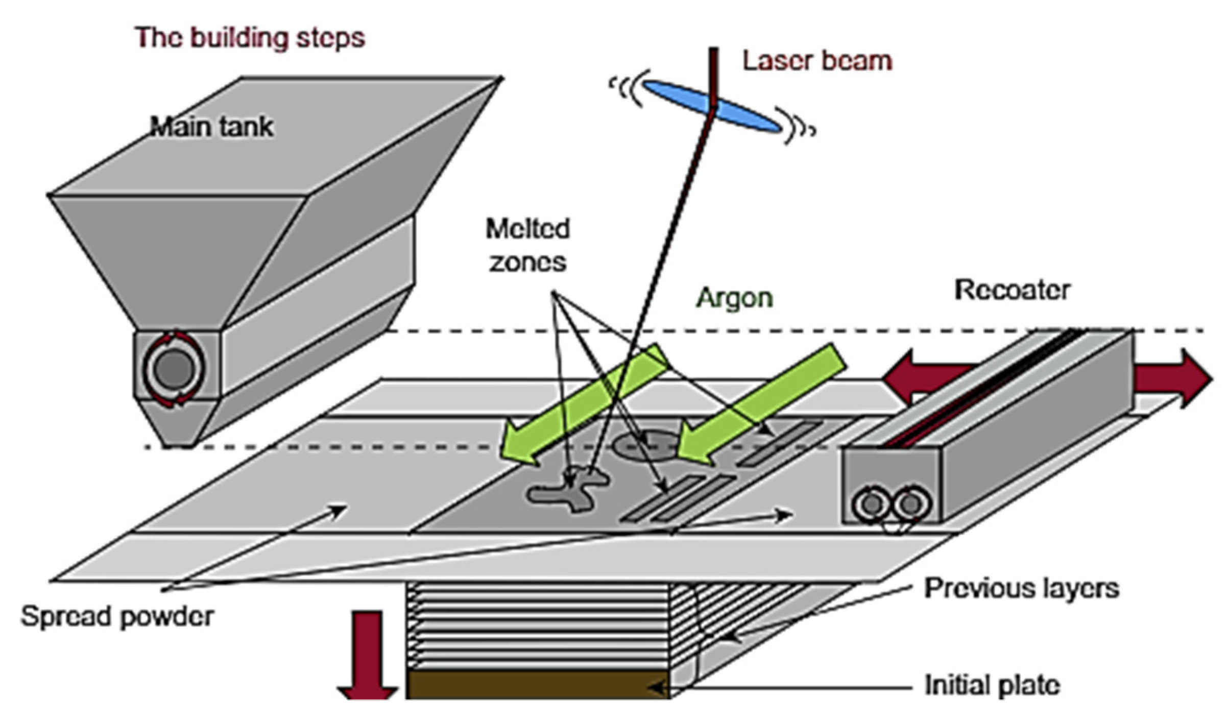
PBF processes are metal-based AM where the laser beam scans at a controlled speed selected locations of a powder bed and then fuses the powder to obtain solid material [13] layer by layer by either partial melting, such as in SLS, or full melting, such as in the metal-based process SLM [6]. Reference [13] presents Figure 2, which illustrates the elements of laser-based PBF process.
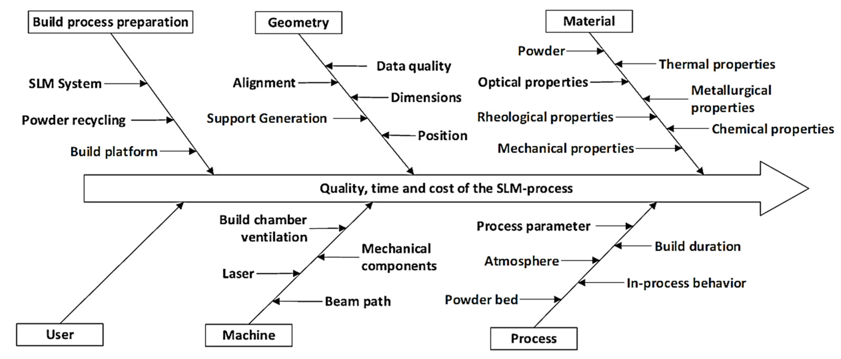
The first crucial part of the SLM process is the build job preparation for any given 3D model. It consists of four main steps: geometry importation, alignment/orientation within a build envelope (critical as surfaces with an angle less than 45° need to be supported), support creation to allow stable processing conditions, and finally slicing based on machine-specific requirements. After preparing and loading a build job onto a machine, the manufacturing process can be initiated starting with the alignment of the recoating device or levelling of the substrate to enable the deposition of powder. Next, the laser scans a specific area based on a predefined scanning strategy and controllable parameters to selectively solidify the material. After finishing a layer scanning, the build plate is moved down, and new powder is deposited on top of the build area to produce a new layer [14]. Reference [14] presented Figure 3 that illustrates the influential factors of a typical SLM process:
There are many applications of the SLM process in real life, such as in the medical field with dental implants (highly complex, small in dimension, and one-off patient products) or with specialized surgery equipment. Another large field is in the aerospace industry where it is hard to manufacture materials, such as nickel-based superalloy, and requires high quality, complex shapes, and low to medium production lots like hydraulic manifolds [14].

2.2. Thermodynamical Phenomena

The PBF process involves complicated thermodynamical phenomena and physiochemical behavior, as powder particles are melted using a laser beam with high energy. Thermodynamic monitoring is important to control the performance of the process, but it is difficult as the molten pool is small and moves quickly. Recently, numerical modelling has been developed to study the physical mechanism deeply. Metal SLM involves principles for multiscale coordinate control, and they include deformation and stress (macroscale), melting behavior and laser absorption (mesoscale), and the development of microstructure (microscale) [15].
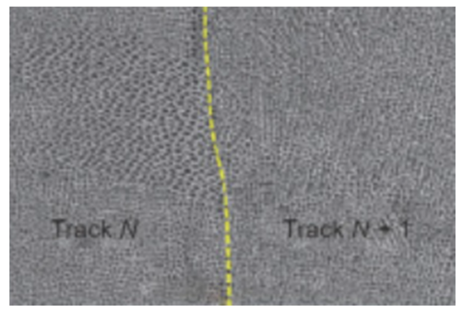
The limited energy on the powder bed and low operating temperature resulting from low laser power value in SLM lead to generating residual pores between the neighboring small molten pools. The low temperature decreased the liquid surface tension, leading to the melt flow [15]. These conditions cause a remarkable reduction of the melt pool convection, and simultaneously lead to a weakening of the melt migration between the current and solidified neighboring tracks. As a result, the porosity is shown obviously on the top surface and cross-section of the SLM part. Conversely, increasing the laser power results in a larger molten pool size with a longer lifetime of the liquid. The considerable laser energy input leads to an intensified convection within the melt pool with sufficient melt migrations between the high laser power tracks, which produce high-quality SLM parts without distinct defects on both the cross-section and top surface. In addition, cellular morphology is presented with the microstructure surrounding the tracks with no obvious defects. Reference [15] presented the following Figure 4 and Figure 5 for the top surface morphology of the produced Inconel 718 part with two different laser powers, 90 W and 120 W.
Therefore, with a low laser power value of 90 W, irregularly shaped porosity was shown distinctively in the tracks where heat transfer and limited mass occurred. Increasing the laser power value to 120 W decreased the porosity. Therefore, producing high-quality Inconel 718 parts are achievable with optimal laser power that can be specified using mesoscale simulation and analysis [15].

2.3. Parameters

The process parameters for PBF can be classified into four categories. The first one is the parameters related to the laser which include laser power, spot size, wavelength, pulse frequency, and duration. The second category is scanning strategy parameters (scanning speed, scanning patterns, scanning spacing, and layer thickness). The third category is the set of powder-related parameters which include powder bed density, particle shape, distribution and size, material proprieties, and layer thickness. The last category is the parameters related to temperature, including the temperature of the powder bed and feeder and temperature uniformity [13].

2.4. Open Issues

Metal-based AM has many gaps that need to be addressed, such as porosity, cracks, and part deformation [6], but as mentioned previously, porosity is a challenging issue due to its effect on the mechanical properties, structural integrity, strength, and Young’s modulus of the produced material. There are three main pore types, namely gas, keyholes, and lack of fusion pore [7]. The following subsection will explain each type, showing its characteristics and mechanism of formation.

2.4.1. Gas Porosity

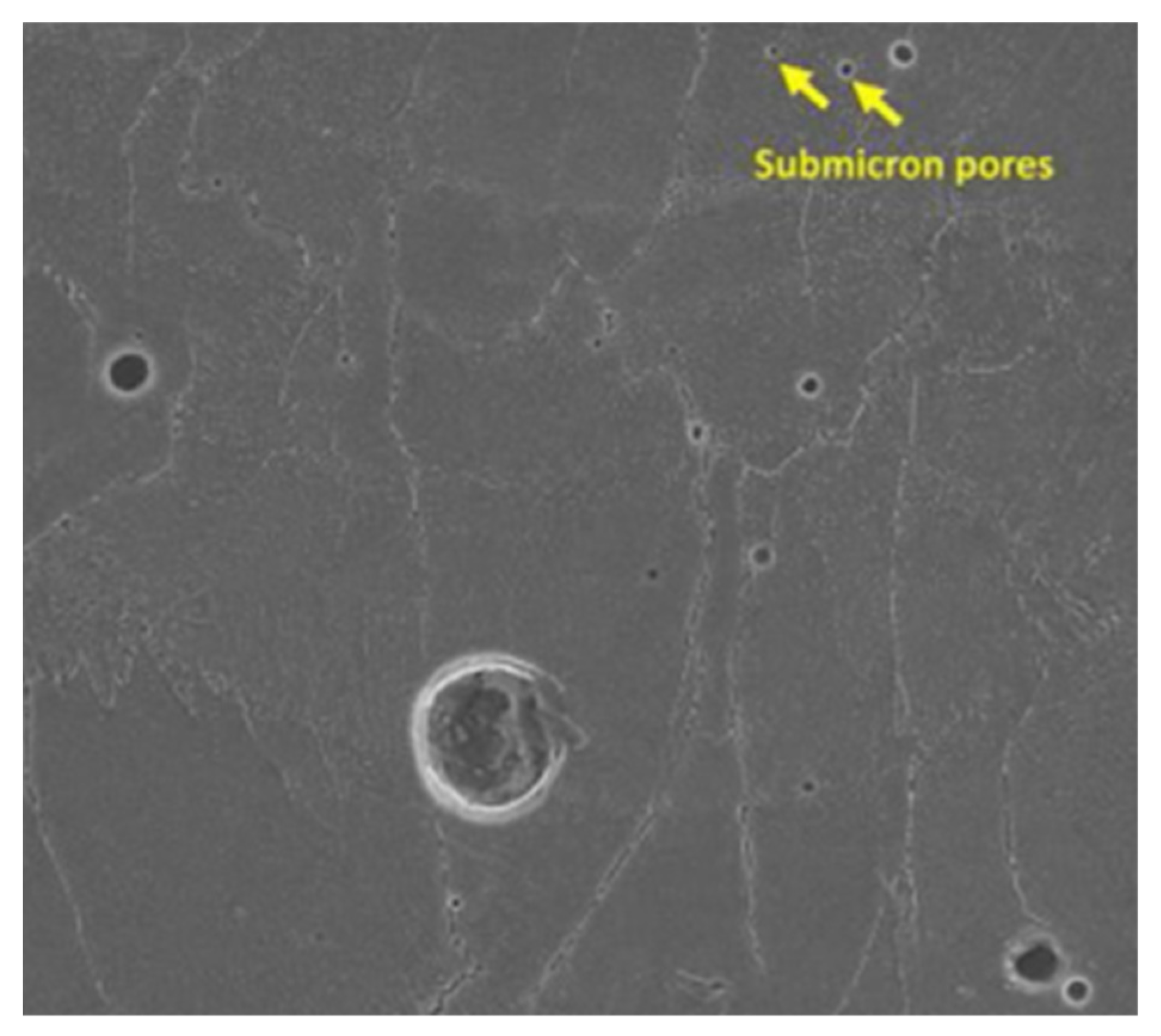
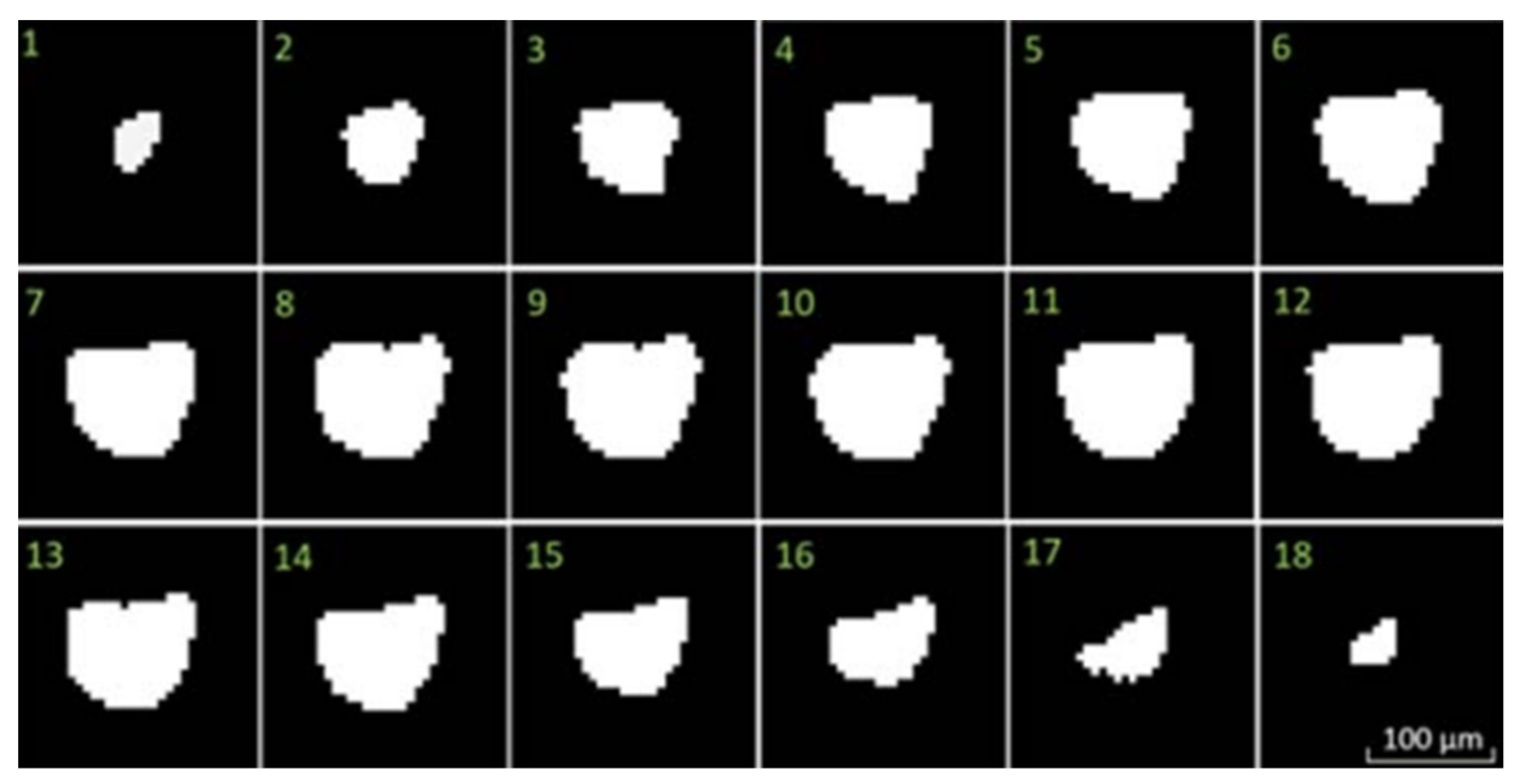
Gas pores belong to the most common type of pores. They are the most spherical and the smallest type. It is characterized by smooth edges and a wide range of sizes from submicron to several microns [16]. The following Figure 6 shows an illustrative example of the gas porosity using the scanning electron microscope (SEM) [16]:
Gas pores are connected to trapped gas that might have different sources of origin, either during or before the process starts, such as the entrapped gas in the powder of the alloy during the process of gas atomization. However, increasing the laser power or decreasing the scanning speed might enlarge this type of pore. Reference [16] fabricated SLM samples at a specific scanning speed of 1200 mm/s and with laser power values between 225 W to 375 W to investigate the gas porosity evolution. They found that increasing the laser power from 225 W to 300 W leads to raising the fraction of gas pore from 1.3% to 1.6% but increasing the laser power further from 300 W to 375 W reduced the fraction to 0.7% as the thermal gradient between the center and boundary of melt pool is increased, which leads to facilitating the process of outgassing. Therefore, it was concluded that it is difficult to fully understand the effect of SLM process parameters on gas porosity formation, since it is a dynamic process that involves pore nucleation, growth, and outgassing during rapid solidification [16].

2.4.2. Keyhole Porosity

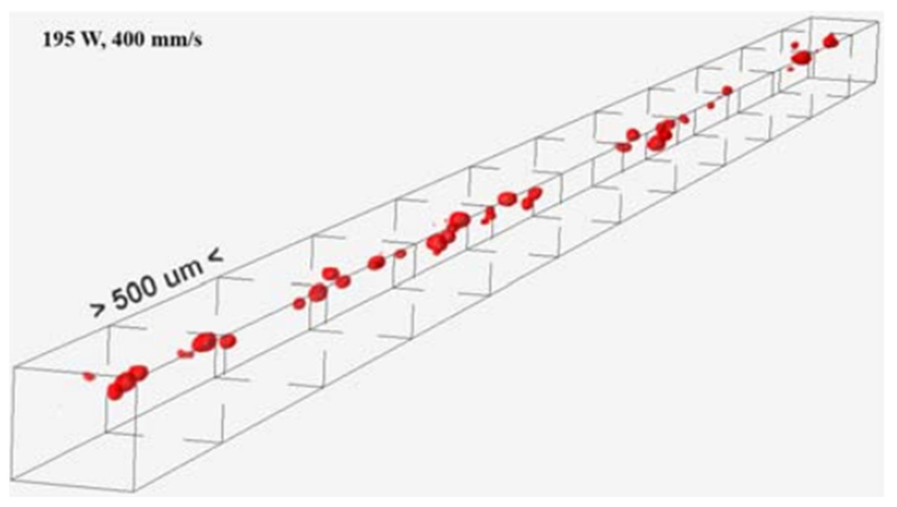
Keyhole pores arise from energy input excess with an energy density value of more than 110 J/mm3 [16], which is a result of increasing the laser power or decreasing scanning speed. It is characterized by large-size cavities reaching hundreds of microns and tended to be near-spherical in shape, so sometimes it is difficult to distinguish between large gas pores and keyhole pores. The following Figure 7 and Figure 8 show the 3D view of the keyhole pore at a laser power value of 195 W and scanning speed value of 400 mm/sand different shapes of 2D images [6].
Unlike gas pores, the surface and contour are bumpy, and these cavities are the most common type of keyhole porosity that appear in the SLM part [16]. It is caused when trapping bubbles of vapor within the melt pool [6], changing the melting mode from conduction to keyhole mode at high laser energy intensity leads to the formation of this type of pore. In the conduction mode, the laser energy input is low to moderate which mediates the heat transfer through conduction. The material melting happens in this mode without vaporization which results in less porosity, but in the keyhole mode, the high laser intensity causes metal evaporation which generates recoil pressure at the bottom of the melt pool. The instability of the dynamic behavior in the melt pool leads to the formation of keyhole porosity with near-spherical morphology at the bottom of the melt pool, which acts as a stress concentrator, causing material property deterioration [16].

2.4.3. Lack of Fusion Porosity

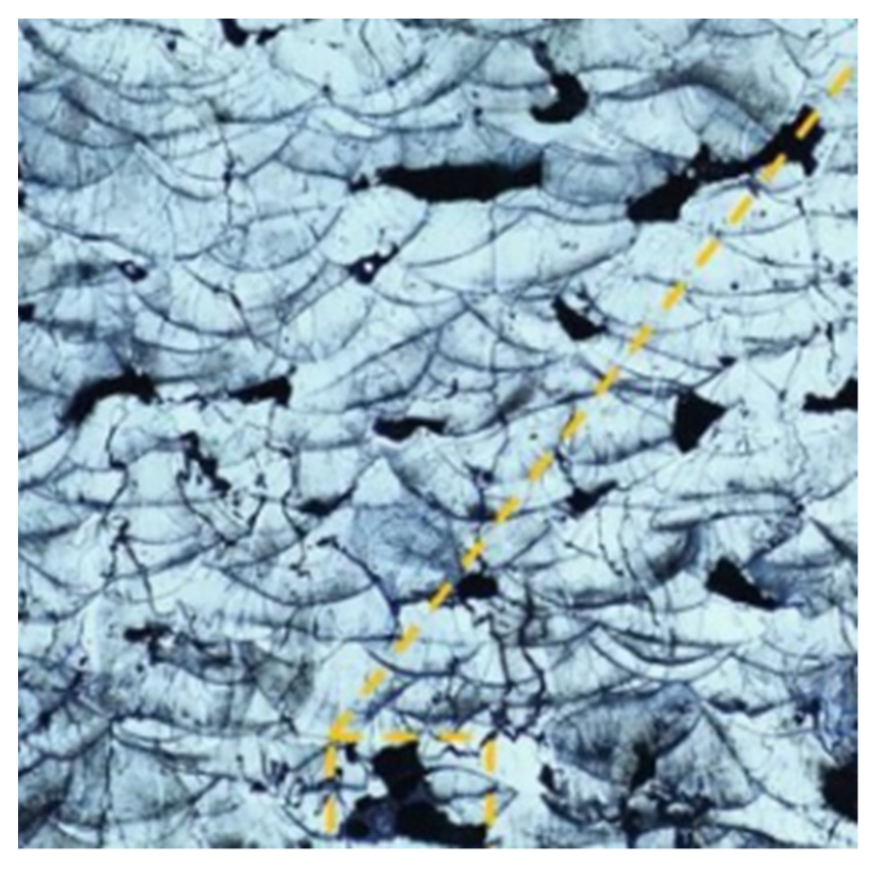
Lack of fusion pores have irregular voids morphology that commonly appeared in SLM alloy. They are featured with large sizes, reaching hundreds of micrometers as shown in the following Figure 9 [16]:
Irregular voids are formed because of un-melting in some regions caused by the reduction in energy density, which is generally a result of the low value of laser power or fast scanning speed [16]. The energy density is a function consisting of laser power, scanning speed, layer thickness, and hatch distance, and these parameters have a significant effect on pores formation [6]. Having insufficient laser energy to induce the overlapping between the adjacent layers leads to the formation of this type of pore. Additionally, the high reflectivity and dense oxide presence on the powder particles’ surface might form such defects as the laser penetrability is lowered [16].
Thus, when optimizing the SLM process, it is essential to accurately study the pore formation occurring when using various combinations of parameters.

2.5. State of the Art Studies

Detecting porosities in PBF processes has a significant contribution to improving part quality [17]. The porosity during the laser additive manufacturing process was monitored using a deep learning-based method, namely convolutional neural network, that predicts the porosity based on melt pool cross-section images acquired by coaxial camera [18]. The model achieved an accuracy of 91.2% in detecting porosity occurrence, and all misclassified samples have pores less than 50 µm. This limitation in detecting micropores is one of the issues in applying convolutional neural network for pores prediction. Similarly, a lack of fusion porosity was predicted based on melt pool data collected during the selective laser melting process, and the DMP monitoring system was used to monitor the melt pool during the processing with titanium alloy material. Next, they created an algorithm that correlated the porosity with melt pool monitoring data, which achieved 90% prediction sensitivity for events with a lack of fusion pores greater than 160 µm volume [19].
Recently, acoustic signals have been used in porosity classification, particularly in achieving the balance between classification accuracy and spatial resolution in porosity detection. High sensitivity fiber Bragg grating sensor was adopted to collect acoustic signals for airborne. The time span for each running window was 160ms, and 300 patterns represented each of the three porosity levels without overlapping between training and testing set in terms of the running window. The parts with different porosity levels were classified using spectral CNN with a classification accuracy between 83–89% [20].
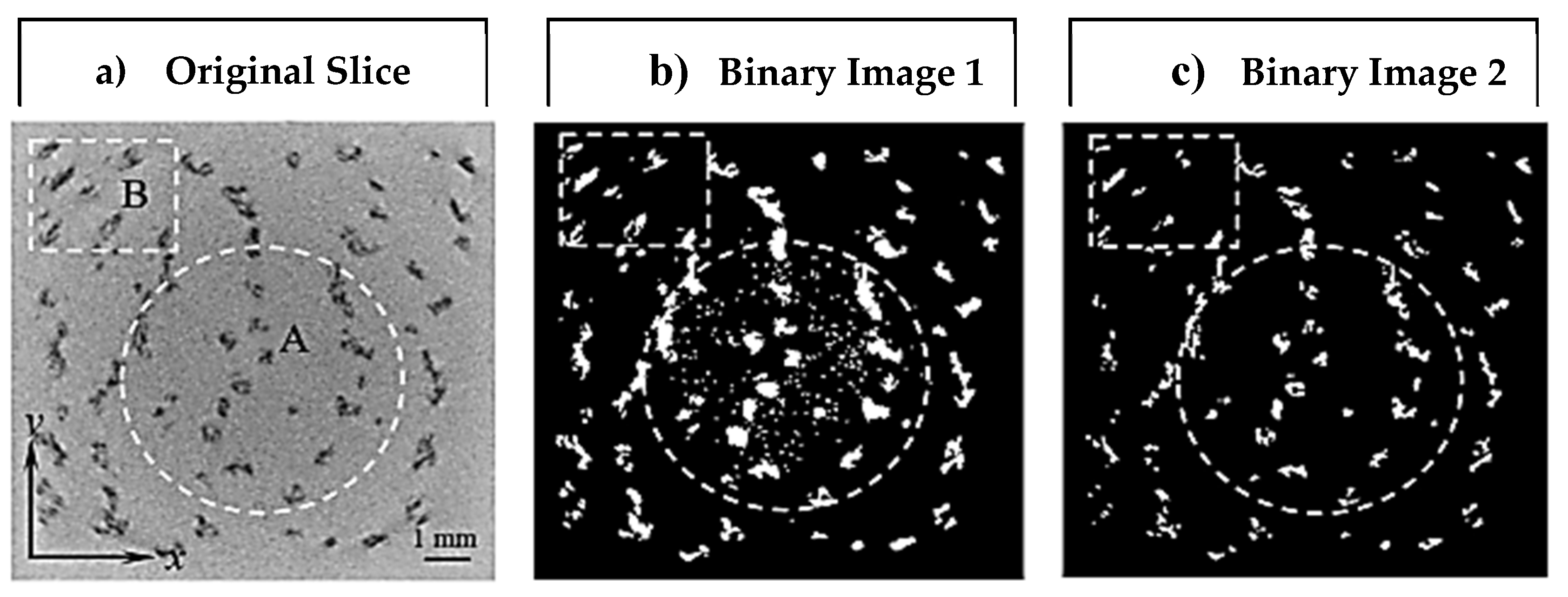
Using CT scans of sample parts, there is a problem related to assessing accurately the porosity in SLM parts [21]. One main drawback is clear when using gray value analysis to assess the porosity of SLM parts visible in CT scan slices. The difficulty is the subjectivity in selecting an appropriate grayscale threshold that would convert a single slice into binary images highlighting defective regions, as well as determining the true level of porosity. For example, in Figure 10 when an inappropriately low grayscale threshold is used for binary image conversion for the original slice, an amount of tiny undesired white spots is not filtered, as shown in Figure 10b. However, adopting a high threshold causes significant alterations in the morphological features of the defective area, more specifically near the boundary, as shown in Figure 10c. These thresholds would result in significantly different predictions of porosity levels.
To evaluate this issue further, the authors of this study [21] proposed an empirical method to estimate the porosity in finished SLM parts using a naturalized threshold for CT scan slices. When compared with the Archimedes method, they found similar increasing or decreasing trends in the predicted percentage of porosity, and concluded that the naturalized greyscale threshold is not the best method for porosity estimation in CT scan slices due to radiodensity variation and CT setup mutual influence. Thus, compensating for these variations is difficult with a unique grayscale [21]. This limitation is found in one of the main existing methods used in porosity estimation, along with the Archimedes method, as mentioned in [22]. Thus, this paper addresses this gap by proposing a new approach based on the use of a Regression Convolutional Neural Network (RCNN) algorithm to predict the percent of porosity in CT scans of finished SLM parts, without the need for subjective difficult thresholding determination to convert single slice to a binary image. In order to test the algorithm, as the training of the RCNN would require a large amount of experimental data, artificial porosity images mimicking real CT scan slices of the finished SLM part will be created using a new efficient method explained in detail in the following section.

3. Artificial Porosity Images Creation for SLM Parts

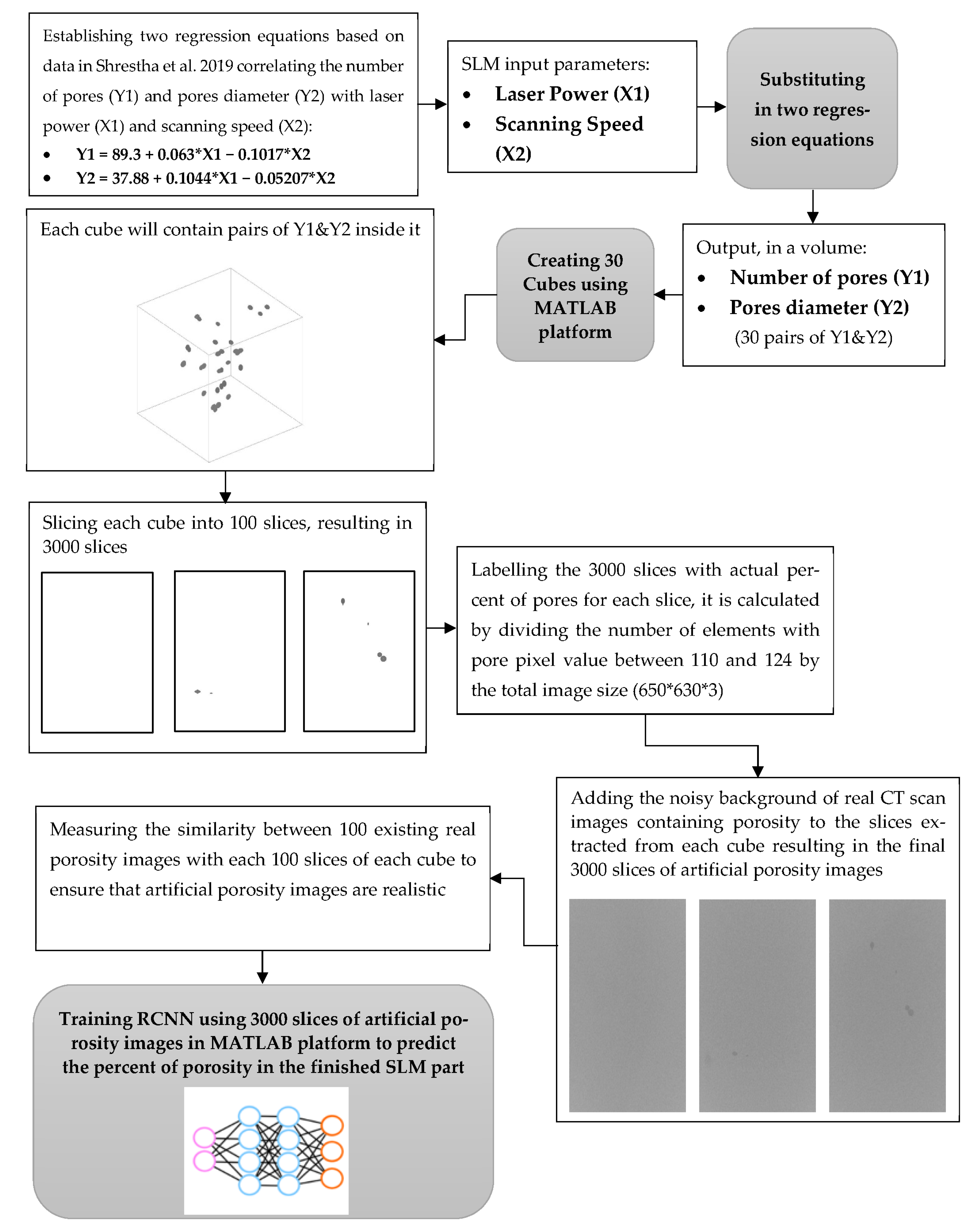
Training CNN algorithms would require a large amount of experimental data, which is expensive for SLM parts [23], since there are many types of production costs for pre-processing, processing, and post-processing costs, including preparing geometry data, CAD model, machine setup, material cost, building up the part, and postprocessing cost [24], so producing a large amount of porosity images to train RCNN is not cost-effective. This section proposes a new efficient approach of creating artificial keyhole porosity images mimicking the real CT scan slices of finished SLM parts that can be used in the research environment effectively and efficiently, in particular to validate the training of an accurate RCNN for the automatic prediction of porosity in CT scans of SLM parts. The steps of creating the artificial porosity images are illustrated in Figure 11, followed by subsections explaining the steps in detail.

3.1. Establishing Regression Equations

The formulation of two regression equations is based on the laser power and the scanning speed data found in [6]. The first equation correlates the number of pores (Y) with the laser power (X1) and the scanning speed (X2), and the second equation correlates the pores’ diameters (Y) with the same parameters (X1 and X2). The data used to establish the two equations are related to keyhole porosity and they will be used as a demonstration for an example of pore types’ formation.
Table 2 shows the corresponding number of pores for each combination of laser power and scanning speed.
The Minitab software was used to establish the first regression equation that fits the 24 observations [6] mentioned in the previous table, thus correlating the number of pores with the laser power and the scanning speed, which results in the following equation:
Number of Pores = 89.3 + 0.063 × Laser Power − 0.1017 × Scanning Speed
Similarly, the second regression equation was established to fit pores diameter with laser power and scanning speed data found in [6], and the dataset is shown in the following Table 3.
Once again, the Minitab software was used to establish the regression equation that fits the 11 observations [6] mentioned in Table 3 correlating the diameter of the pores with the laser power and the scanning speed, which results in the following equation:
Pores Diameter = 37.88 + 0.1044 × Laser Power − 0.05207 × Scanning Speed

3.2. Generating Pores Numbers and Diameters

The two regression equations established in the previous section were used to generate 30 values for the number of pores and pores diameter by substituting the 30 combinations of laser power and scanning speed found in [6]. The following is an illustrative example using a laser power of 15 W and a scanning speed of 50 mm/s:
Number of Pores = 89.3 + 0.063 × (15) − 0.1017 × (50) = 85 Pores
Pores Diameter = 37.88 + 0.1044 × (15) − 0.05207 × (50) = 36.94 µm
Table 4 shows the 30 combinations of laser power and scanning speed found in [6], along with the corresponding number of pores after scaling down from a 2.6 mm3 to a 1mm3 volume, the volume of the cube in which the pores will be positioned and used to train the CNN. Variations of ±10 µm were applied randomly to the generated pore diameters, mimicking variations occurring in real porosity images.

3.3. Creating 3D Cubes

Overall, 30 samples of 3D cubes were created with a volume of 1 mm3 for each cube, and they contain the number of pores with diameters generated in the previous section (Table 4). Thus, the first cube has 33 pores with an average diameter of 36.94 µm. In [25], the position of pores was considered by analyzing the porosity distribution in real images of pores. They observed 975 porosity positions in X and Y. In this research, the Minitab platform was used to conduct a normality test on these observations, as shown in the following Figure 12 and Figure 13:
With a p-value of less than 0.005, the probability that these data are not coming from a normal distribution is very low, so it is concluded that the observed porosity positions are normally distributed, with a mean and a standard deviation of 0.48 and 0.27 for X-positions and 0.44 and 0.26 for Y-positions. Therefore, in this research, it was decided to produce porosity positions with the same statistical distribution, as observed in [25].
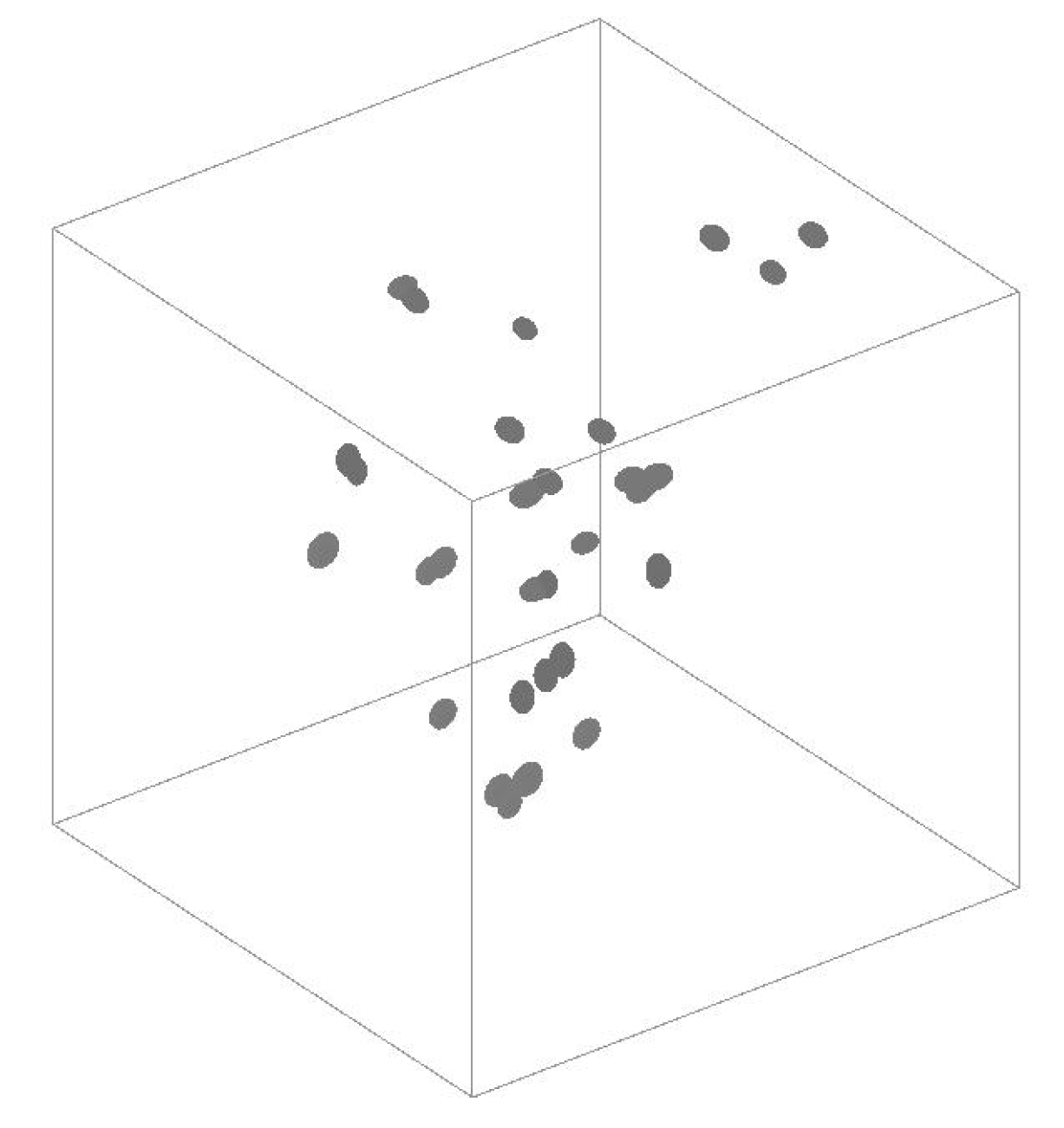
Thus, MATLAB software was used to generate normally distributed porosity positions inside each of the 30 cubes with the mean and the standard deviation mentioned previously in the X and Y positions, while the Z position was arbitrarily given the average between X and Y to produce normal distribution positions in a volume. The pores morphology was created to be similar to the 3D view of the pores shown in Figure 7 in Section 2.4.2 [6]. The following Figure 14 shows an illustrative example of the cube with 33 pores and an average diameter of 36.94 µm, as mentioned in the first combination of Table 4.

3.4. Slicing 3D Cubes into 2D Images

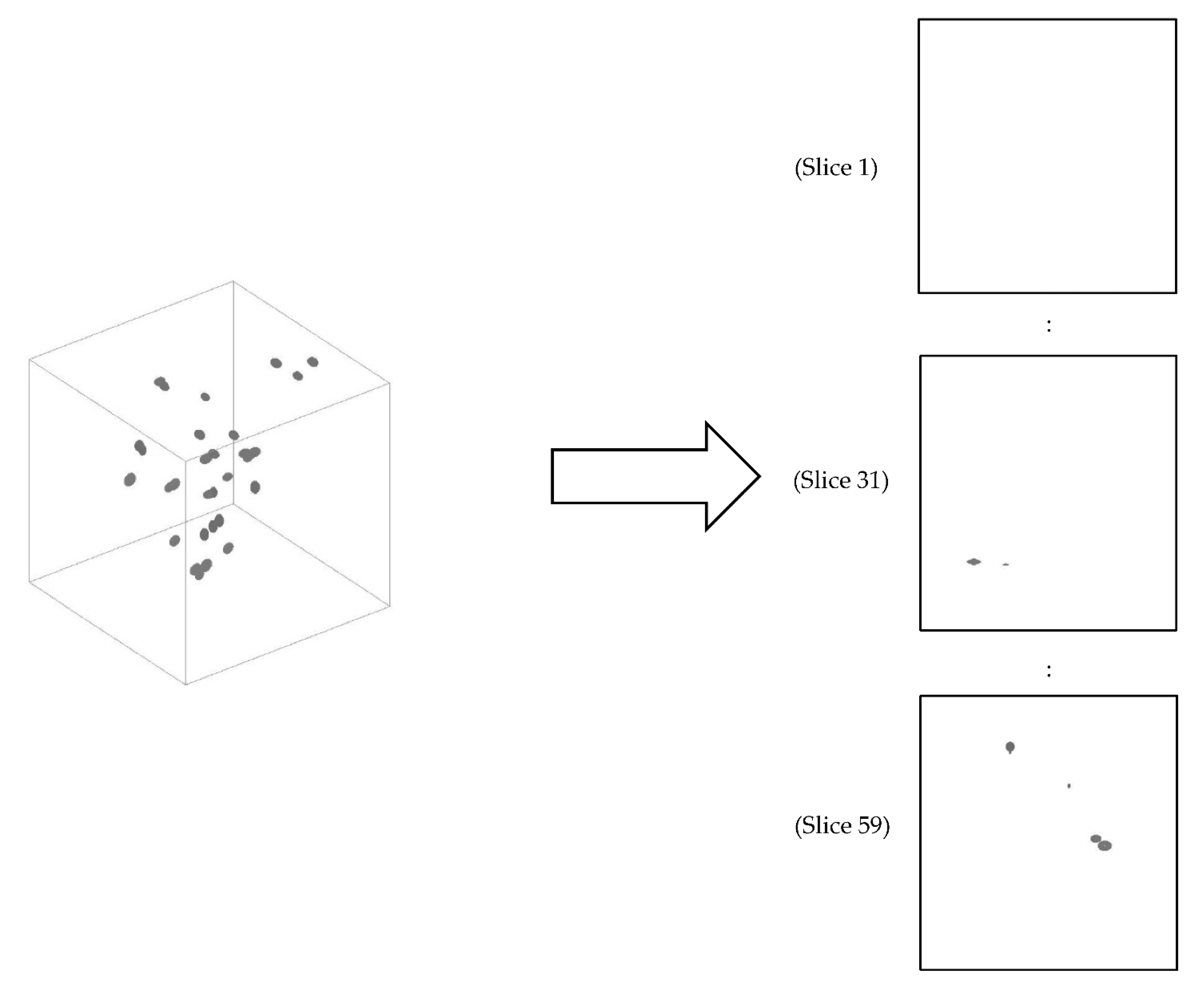
Each cube created in the previous step was sliced using the MATLAB platform into 100 slices with a thickness of 0.01 mm, resulting in 3000 slices of 2D images, an illustrative example of the cube, and three non-sequential slices that are shown in the following Figure 15.
The first slices are expected to be with no pore, as shown at the bottom of the cube. Thereafter, part of a pore is shown in some slices and parts of many pores are shown in other slices. The pore morphology tended to be near-spherical in shape, as described in Section 2.4.2 [16].

3.5. Labelling 2D Slices

The slices were labelled with the actual percent of porosity for each slice using MATLAB software, and were calculated by dividing the number of elements with specific pore unique pixel values by the total image size (650 × 630 × 3). The pixel values for the pores were determined by inspecting the pixel values of porosity seen in real CT Scan images [26], and are between 110 and 124. The first slice has no elements with a pixel value in the range between 110 and 124 so the actual percentage of pore is 0. In slice 31 there are 258 elements with pixel values in the range specified, so the actual percent of pore is (258/(650 × 630 × 3)) × 100 = 0.0210, similarly for slice 59 with 2193 elements of pixel values between 110 and 124, the actual percent of pore is (2193/(650 × 630 × 3)) × 100 = 0.1785, and the average actual percent of pore for 3000 slices is 0.0134.

3.6. Adding Noisy Background

Firstly, image processing in the MATLAB platform was conducted to fuse the noisy background of 100 CT scan images containing porosities with the slices extracted from each cube, resulting in the first version of the filtered artificial images shown in the following Figure 16.
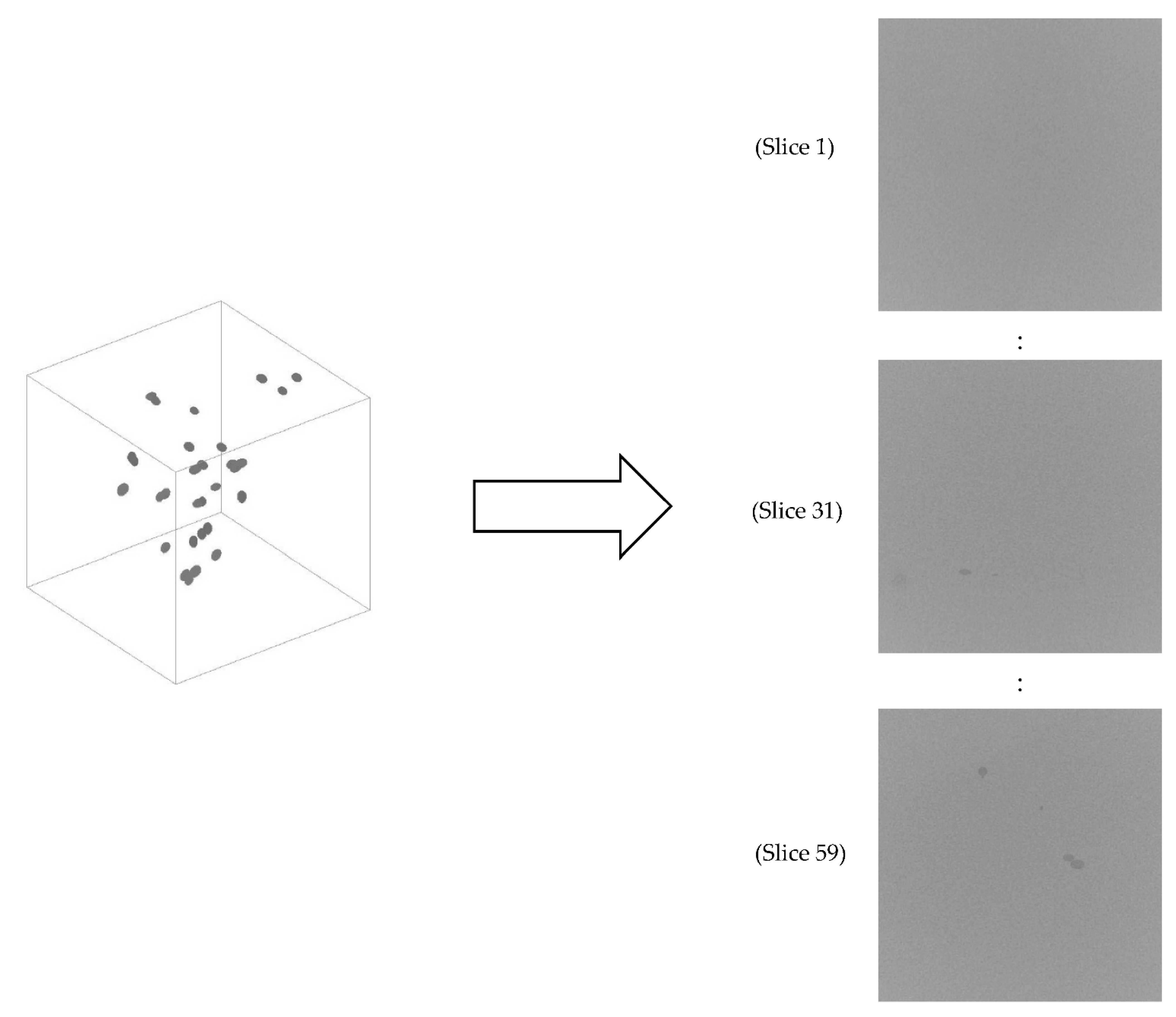
Secondly, in the artificial images, the edges of the pores have a uniform shading, making them clearly distinguishable from the background. This is not a true representation of porosity seen on real CT scans, where shade variations make it difficult to properly distinguish pores’ edges. Thus, in a second version, image processing in the MATLAB platform was conducted to further filter the artificial porosity images by creating similar noise, so the background of a sample of 100 existing images was inserted into 100 pores slices extracted from 3D cube after reducing the pixel value for its white background from 255 to 155 to convert it to a gray background. The artificial images were overlayed with the noisy background of real images. The degree of overlaying was determined by a factor (between 0 and 1) following the method described in [27].
Thus, with a factor of 1, the pore image will be shown without noisy background and with a factor of 0, and the noisy background will be shown without pores. After many trial and error experiments, a factor of 0.125 was considered to visually be the best value that combined both pore and noisy background images, as shown in the following Figure 17.
As shown in the slices, the noise in the background and the pores appear more like real porosity images as the edges are not as clearly defined, but this is a subjective evaluation. The following Section 3.7 will present quantitative measure for the similarity between real and artificial porosity images to ensure that the artificial images are realistic.

3.7. Measuring the Similarity between Artificial and Real Porosity Images

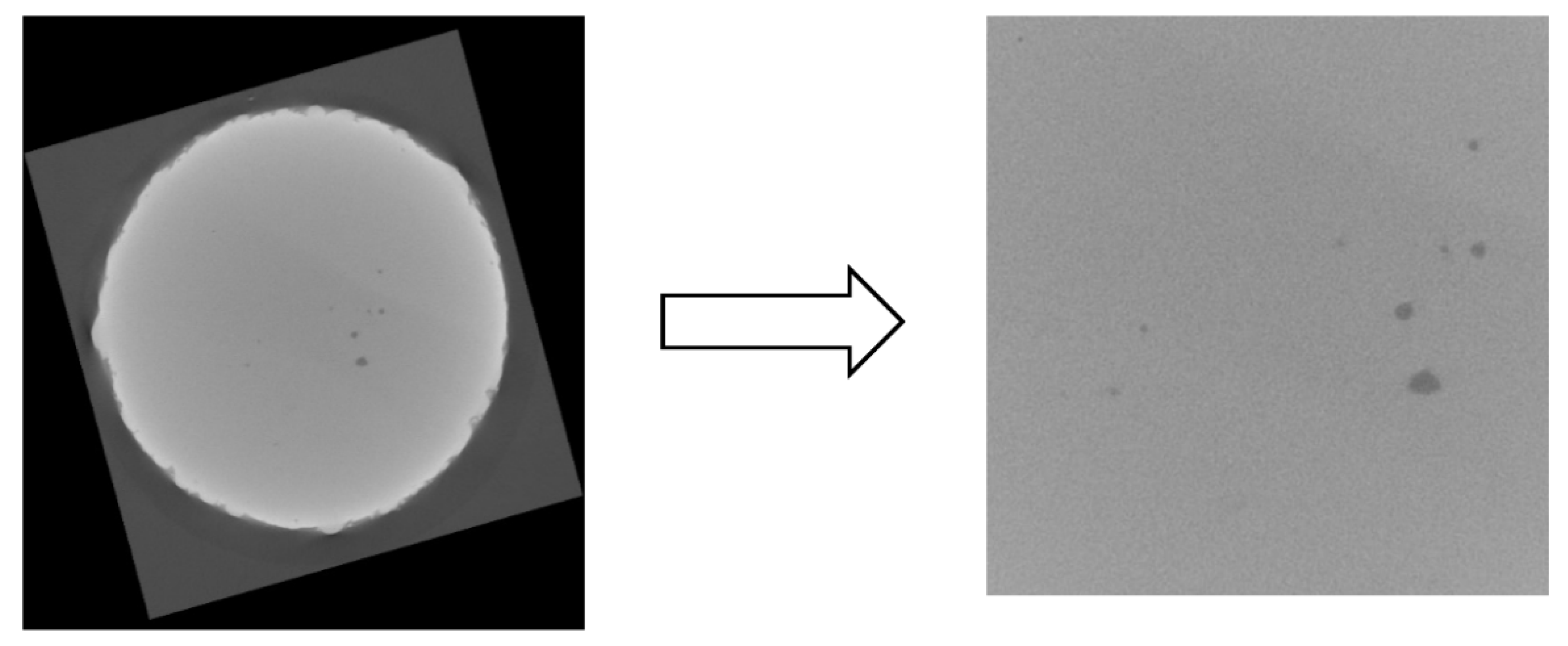
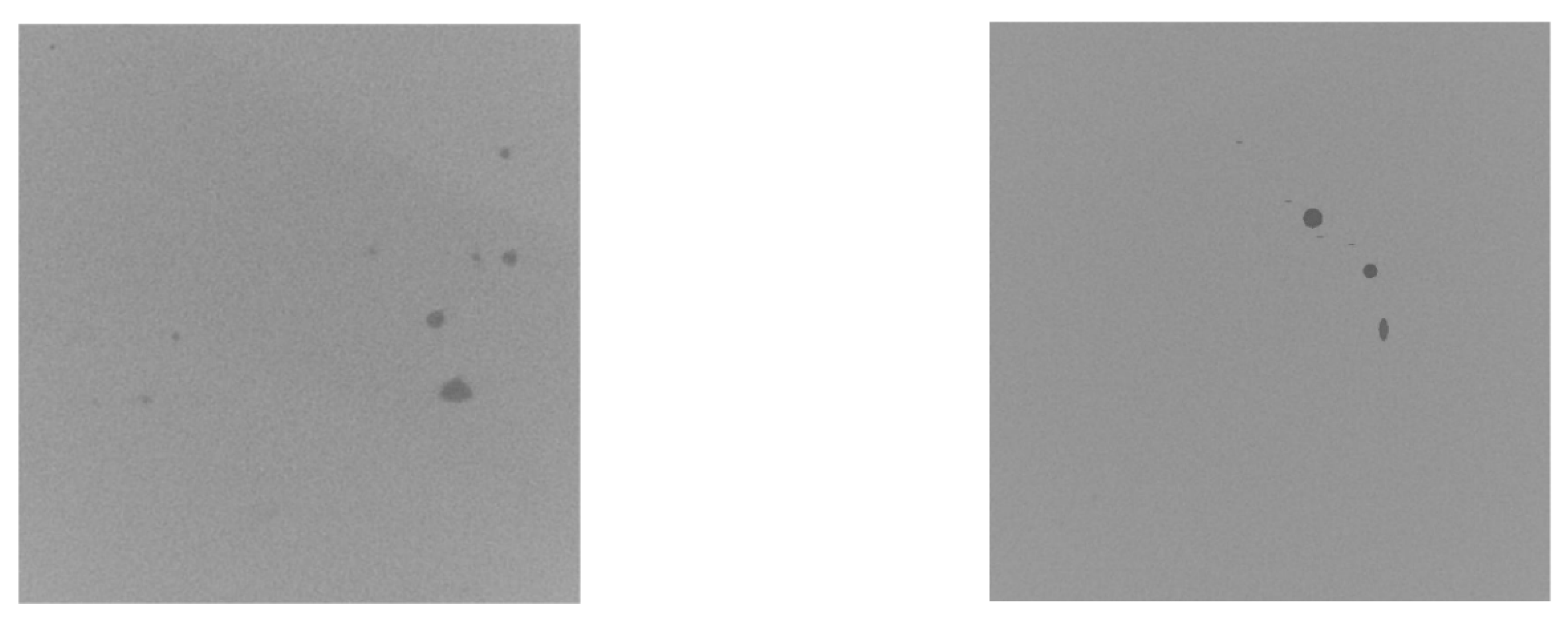
The created artificial porosity images were compared with real CT scan slices of finished SLM parts [26] to verify that the simulated images are close the reality. The real images are only used as a demonstration and are not directly linked with the pore formation equations mentioned in Section 3.1. The following Figure 18 shows an illustrative example of the slices before and after processing, which was required to focus on the bulk of the material and to obtain images of the same size as the artificial images.
Figure 19 presents the real image along with the first version of the artificial image.
Samples of 100 slices of real images were taken and compared with each of the first versions of 100 artificial images created in the previous section. The comparison was made using a quantitative method called Structural Similarity Index (SSI). It is a measure that assesses the images based on three computational terms, namely the luminance (l), the contrast (c), and the structural terms (s). Multiplying the three terms results in the overall index. If two images are exactly the same, the index should be 1, and if they are totally different the index should be close to zero. The mathematical equations for calculating SSI for images x and y are as follow [28]:
SSI(x,y) = [l(x,y)]α × [c(x,y)]β × [s(x,y)]γ
where:
l(x,y) = (2 × µx × µy + C1)/(µx2 + µy2 + C1)
c(x,y) = (2 × σx × σy + C2)/(σx2 + σy2 + C2)
s(x,y) = (σxy + C3)/(σx × σy + C3)
µx and µy are local means, σx and σy are standard deviations, and σxy is cross-covariance for images x and y. The exponents for luminance, contrast and structural are alpha(α), beta(β), and gamma(γ), while C1, C2, and C3 are constants added to avoid instability for image regions with local mean or standard deviation close to zero.
MATLAB software was used to calculate SSI between the real and first version of artificial porosity images, the average similarity index for 3000 slices was 0.9586. The same 100 samples of real images were used to compare them, with the final version of artificial porosity images shown in the following Figure 20:
The average similarity index for 3000 slices was improved to 0.9967, which means that the final version of artificial porosity images mimics better real images since the index is closer to 1.

3.8. Study Limitations

The created artificial porosity images in this section will be used only to test the proposed CNN algorithms that will be developed in Section 4. The study did not aim to study the porosities in depth, so no experiments have been conducted, but the paper proposes a method that will enhance such studies, particularly in predicting the percent of porosity as will be demonstrated in Section 4. In the future, real experiments can be conducted in order to produce real porosity images.

4. Predicting the Porosity in Selective Laser Melting Parts

Using the artificial images created in Section 3, this section will show three methods for predicting the percentage of porosity in SLM parts. The first one is the existing image binarization method, which is one of the main methods for measuring porosity along with the Archimedes method [22]. Archimedes’ principle might be used in the case of producing real SLM parts, and this paper uses artificial porosity images, so the image binarization method will be conducted and explained in Section 4.1. The second and third methods are Regression Convolutional Neural Network (RCNN) and hybrid Bees Regression Convolutional Neural Network (BA-RCNN), which will be explained in detail in Section 4.2.

4.1. Predicting the Porosity Using Image Binarization

There is a problem related to accurately assessing the porosity in SLM parts [21]. The problem is the difficulty and subjectivity in selecting an appropriate grayscale threshold for binary image conversion to highlight defective regions and determine the true level of porosity, as mentioned previously in Section 2.5.
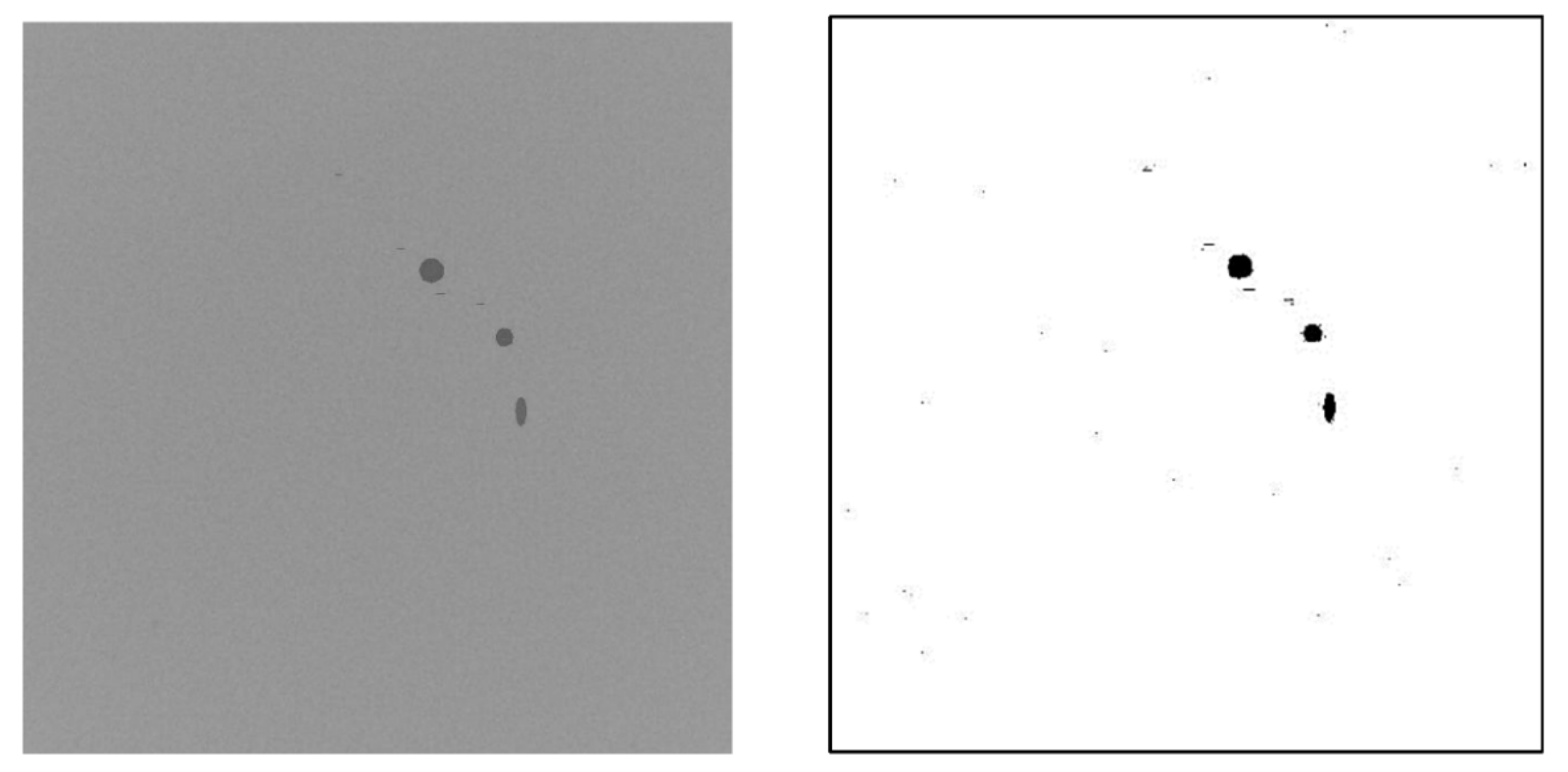
The first version of created artificial images presented in the previous section were binarized using an adaptive thresholding algorithm provided in the MATLAB platform, which selects the threshold based on local mean intensity in the pixel neighborhood, and is determined by a sensitivity factor, between 0 and 1, that indicates the sensitivity toward thresholding more pixels as a foreground [29]. This sensitivity factor is selected manually. The following Figure 21 shows the first version of the artificial image, along with the binarized image with an arbitrarily selected sensitivity factor of 0.66.
As can be seen in the figure, there are tiny undesired black spots in different positions in the binarized image, and the undesired spots also appear in slices with no pores, as shown in the following Figure 22.
The average actual percent of pore for 3000 slices was 0.0134, while the average percent of pore for 3000 binarized images is overestimated with a value of 0.0578, so the absolute error is 0.0444. The prediction accuracy with a difference of less than a threshold of 0.02 (percent of observations with error less than 0.02) is 64.47%.
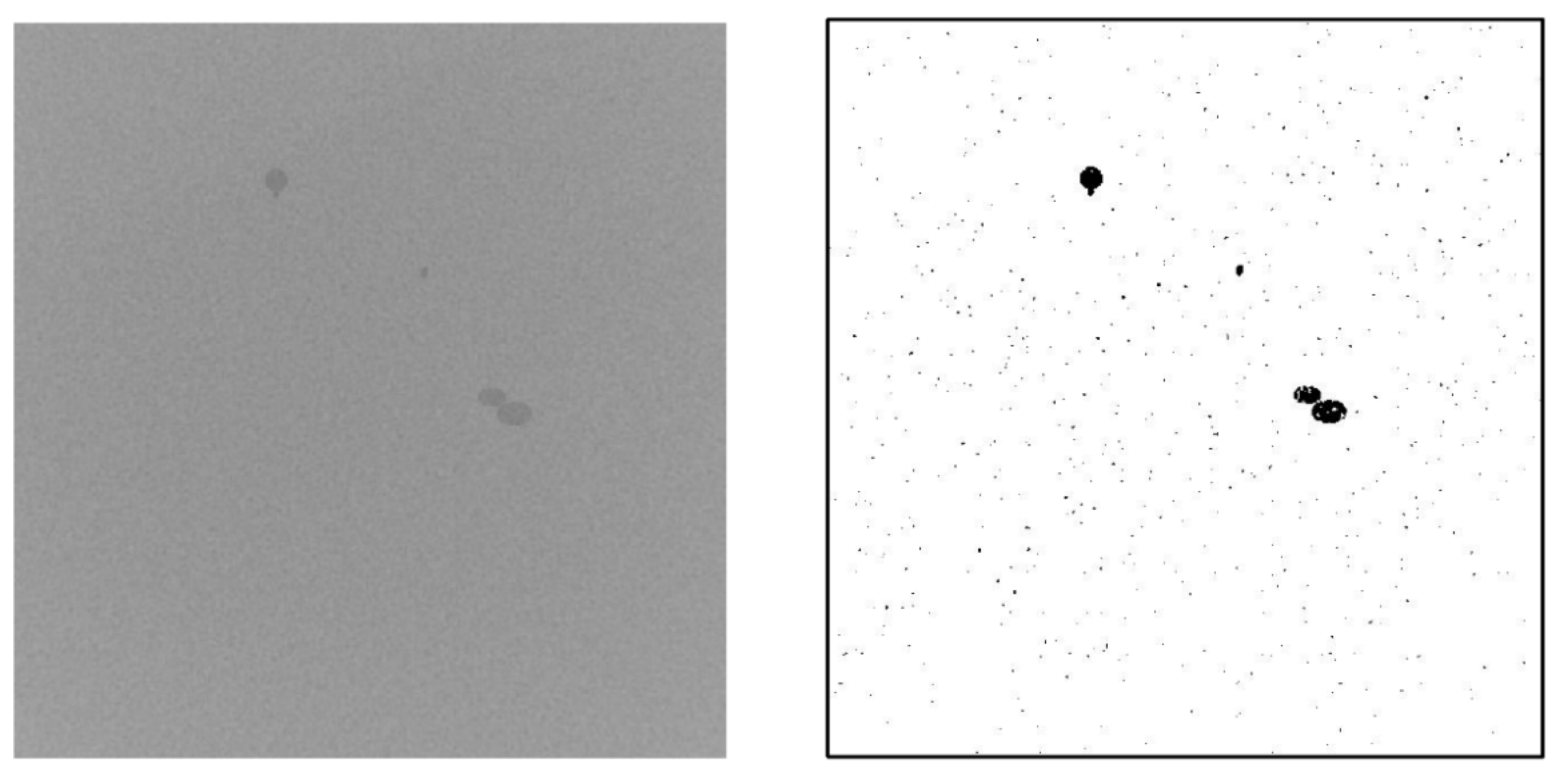
The same approach was followed for the final version of artificial porosity images, and the following Figure 23 shows the artificial image along with the binarized image, with a sensitivity factor of 0.66.
As can be seen in the figure, there are tiny undesired black spots in different positions in the binarized image, confirming the problem stated in [21], which is a result of inconsistent grayscale in CT scan slices because of the mutual influence of CT setup and radiodensity variation. Removing these spots using image processing is time-consuming since they appear in different positions in each slice without a simple pattern, so the processing needs to be performed image by image to distinguish between the undesired black spots and the pores first. Following that, unwanted spots need to be replaced with a white background because they are counted in the porosity calculation which overestimates the percent of porosity. Such an issue also occurs in the pores, as tiny white spots would alter their morphological feature and slightly reduce the percentage of porosity. However, the effect of this on porosity calculations is negligible when compared to the effect of the small black spots occurring in the large background. Depending on the sensitivity factor used, the black spots also appear in slices with no pores, as shown in the following Figure 24.
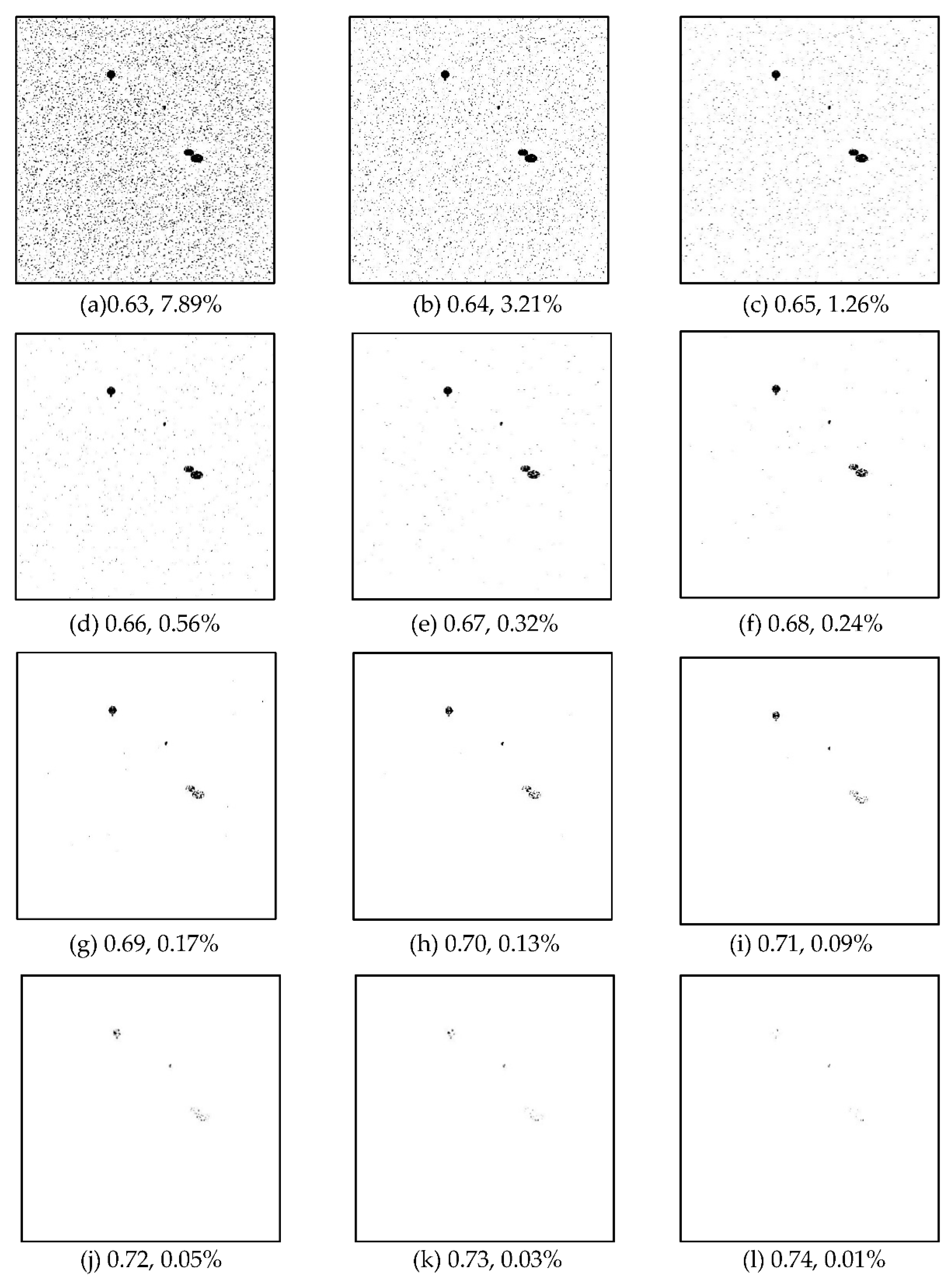
Experimenting with different sensitivity factors between 0.63 to 0.74 resulted in the following binary images with different percentages of porosity as shown in Figure 25.
As can be seen from the images, increasing the sensitivity factors reduces the black spots resulting from the noisy background, but it alters the pore’s morphological features dramatically. A sensitivity factor of 0.69 seems relatively better and it will be selected to binarize all 3000 slices since it yielded the most accurate percent of porosity of 0.17%, which is close to the actual percent of pore for the original slice with a value of 0.1785%. It is worth noting that in the case of producing real porosity images, sensitivity factor selection will be subjective and difficult since the actual percentage of porosity will be unknown. The average percent of pore for 3000 slices was 0.0203, while the average percent of pore for 3000 binarized images is overestimated with a value of 0.0424, so the absolute error is 0.0221. The prediction accuracy with a difference less than a threshold of 0.02 (percent of observations with error less than 0.02) is 68.60%.

4.2. Predicting the Porosity Using RCNN and BA-RCNN

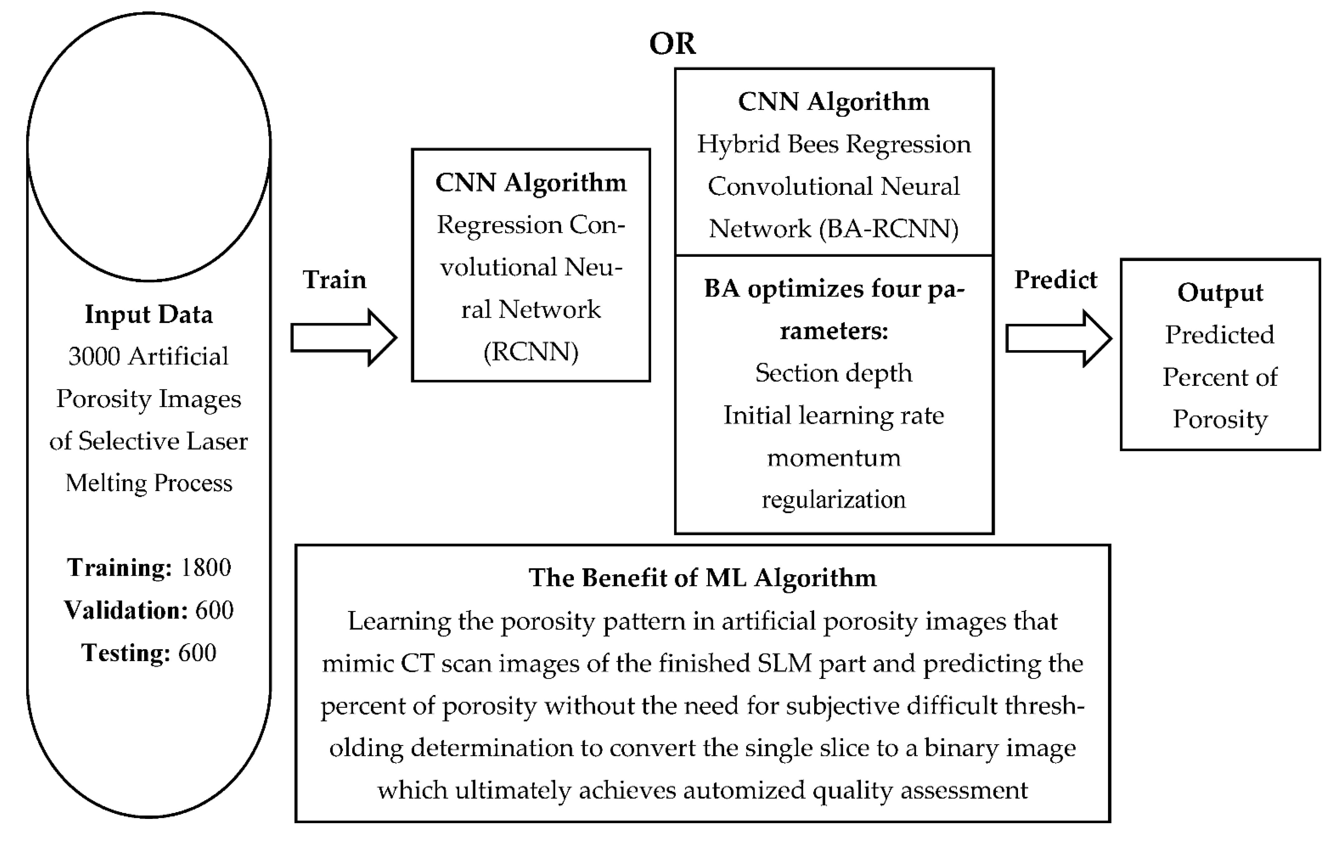
CNN can be used for regression problems to predict numerical values based on images, so regression CNN will be used to predict the percent of porosity based on created artificial porosity images in the previous section. As mentioned previously (in Section 3.5), the images were labelled using the actual percent of porosity calculated during the creation process by dividing the number of elements with specific pore unique pixel values by the total image size. CNN learns the porosity pattern in artificial porosity images that mimic CT scan images of the finished SLM part and predict the percent of porosity without the need for subjective difficult thresholding determination to convert the single slice to a binary image, which ultimately achieves automized quality assessment.

4.2.1. RCNN and BA-RCNN Architecture

The CNN architecture for predicting the percent of porosity is composed of 22 layers with one input layer, five convolutional layers, five rectified linear unit layers, five batch normalization layers, four average pooling layers, one fully connected layer, and one regression layer.
The input layer is represented by a matrix with height by width size (650 × 630). It contains pixel brightness values between 0 for black regions to 255 for white regions. The convolutional layers contain filters represented by weight matrix slide along the pixel brightness matrix using a special dot product to create a feature map matrix [30]. The rectified linear unit layer comes after each convolutional layer to increase the effectiveness and speed of the training by maintaining positive values and mapping negative values to zero [31]. In addition, the batch normalization layer comes after each convolutional layer as a supplement layer mitigating the overfitting risk [32]. Pooling layers are used between the convolutional layers for output dimensionality reduction [33] without losing the important image features, which helps in minimizing the computational time. Regression and fully connected layers are the output layers that show the predicted percentage of pores.
The normal number of convolutional layers to start is between two to three layers with a filter size of 3 × 3 or 5 × 5 as advised in [31], CNN was designed with five convolutional layers with four average pooling layers in between, with the number of filters ranging between 8 for the first layer and 128 for the last one. Each layer has twice the number of filters of the previous layer [34]. The filter size is 5 × 5, the section depth is 3, and the padding that detects the image edges is set as ‘same’, so the padding size is automatically calculated at the training time, producing output size equivalent to input size when the stride (number of pixel shift) is one.
The pooling type is ‘average’ which takes the average presence of the feature, while the max pooling layer takes the most activated feature, so the average pooling is used with light background and max pooling is better with dark background [35], the default size of pooling layer is 2 × 2 [30], but it yielded high computational cost since the image input size is big (650 × 630). The size was changed to 4 × 4 with a stride value of 4 to minimize the training time.
CNN was trained using SGDM, which is the most common training algorithm [32]. The default values for this algorithm are an initial learning rate of 0.01, a momentum of 0.9, a regularization of 1 × 10⁻⁴, and the maximum number of epochs is 20, as presented in [36]. After applying some experiments and monitoring the validation accuracy, the momentum was changed to 0.8, and with regularization became 1 × 10⁻¹⁰.
The RCNN algorithm will train the artificial porosity images of the SLM part to predict the percent of porosity without the need for subjective difficult threshold determination to convert the single slice to a binary image, as mentioned in [21].
The hybrid algorithm (BA-RCNN) uses BA to optimize the parameter values for section depth that controls the network depth, the initial learning rate that is used for features learning, the momentum that performs the hyperparameters update and regularization that prevents overfitting [37] to reach the minimum prediction error on the validation set.
The BA consists of global and local searches. The global search is done by the scout bees that evaluate random positions based on the fitness value. In the local search, the best sites are selected, and the remaining sites are abandoned. The intense search is done to select the elite sites, which are the best among the best sites selected in the local search. The next step is recruiting more bees for the elite sites based on the size of the neighborhood search space and recruiting lower bees for other sites to conduct the local search [38]. The stopping conditions for this iterative process are:
  • Finding the optimal solution
  • Exceeding the iteration number
  • No improvement over specified sequential iterations
The values of BA hyperparameters are assigned based on the capability of the computer and equations in [39]:
  • Scout bees (n) = 4
  • Selected bees (m) = 0.5 × n = 2
  • Elite bees (e) = 1
  • Recruited bees for e (nep) = 2 × m = 4
  • Recruited bees for other best sites (nsp) = 0.5 × n = 2
  • Neighborhood size (ngh) = 0.1 × (Maximum − Minimum):
    Section Depth: 0.1 × (3 − 1) = 0.1 × 2 = 0.2
    Initial Learning Rate: 0.1 × (1 − 1 × 10⁻²) = 0.1 × 0.99 = 0.099
    Momentum: 0.1 × (0.98 − 0.8) = 0.1 × 0.18 = 0.018
    Regularization: 0.1 × (1 × 10−2 − 1 × 10⁻¹⁰) = 0.1 × 0.01 = 0.001
The following Figure 26 shows the pseudo-code for the BA-RCNN algorithm:
The following Figure 27 summarizes the task for hybrid regression CNN:

4.2.2. RCNN and BA-RCNN Results

MATLAB is the platform used to apply RCNN and BA-RCNN on the newly created 3000 artificial porosity images, of which 1800 images are for training and 600 are for each of the validation and testing sets to predict the percent of porosity without the need for subjective difficult thresholding determination to convert the single slice to a binary image, which ultimately achieves automized quality assessment. The following Table 5 shows the average percent of porosity error (the difference between the actual and predicted percent of porosity on average) for the first version of artificial porosity images.
The minimum percent of porosity error value of 0.0160 comes with the validation set in BA-RCNN, and the following Table 6 shows the optimal CNN parameters values optimized using BA.
The minimum error value of 0.0160 was achieved with a section depth of 3, 0.0118 initial learning rate, a momentum value of 0.8229, and a regularization parameter of 0.0091, which is less than the error value of 0.0444 for the image binarization method. The following Table 7 shows the prediction accuracy with a difference less than a threshold of 0.02 (percent of observations with error less than 0.02) for all three sets, along with computational time for all algorithms.
The existing original RCNN produced 78.83% prediction accuracy in the testing set, which is approximately 14% better than the accuracy resulting from the image binarization method with a value of 64.47%. The novel hybrid BA-RCNN produced better prediction accuracy in all training, validation, and testing sets, which means it has better generalization capability than RCNN. The accuracy in the testing set has a value of 80.67%, which is approximately 16% better than the existing image binarization method, and the computational time is almost similar in both algorithms. The following Table 8 shows the prediction accuracy for all three methods.
The same approach is followed to predict the percent of porosity for the final version of artificial porosity images. The following Table 9 shows the average percent of porosity error (the difference between the actual and predicted percent of porosity on average) for the first version of artificial porosity images.
The minimum percent of porosity error value of 0.0214 comes with the validation set in BA-RCNN, and the following Table 10 shows the optimal CNN parameters values optimized using BA.
The minimum error value of 0.0214 comes with a section depth of 1, 0.0101 initial learning rate, a momentum parameter of 0.9568, and a regularization value of 0.0097, and is less than the error value of 0.3167 for the image binarization method. The following Table 11 shows prediction accuracy for training, validation, and testing sets with a difference less than a threshold of 0.02 (percent of observations with error less than 0.02), along with computational time for best iteration for all algorithms.
The existing original RCNN produced 75.50% prediction accuracy in the testing set, which is approximately 7% better than the accuracy resulting from the image binarization method with a value of 68.60%. The novel hybrid BA-RCNN produced better prediction accuracy in all training, validation, and testing sets, which means it has better generalization capability than RCNN. The accuracy in the testing set has a value of 85.33% which is approximately 17% better than the existing image binarization method, and the hybrid BA-RCNN is cost-effective since the computational time is reduced by approximately 2 min. The following Table 12 shows the prediction accuracy for all three methods.
The contribution of the paper is developing a new approach based on the use of a Regression Convolutional Neural Network (RCNN) algorithm to predict the percent of porosity in CT scans of finished SLM parts, without the need for subjective difficult thresholding determination to convert a single slice to a binary image, the model achieved better prediction accuracy than the existing image binarization method by 17%. In order to test the algorithm, as the training of the RCNN would require a large amount of experimental data, artificial porosity images mimicking real CT scan slices of the finished SLM part were created with a similarity index of 0.9976 with real images.

5. Conclusions

Assessing the porosity in Selective Laser Melting (SLM) parts is a challenging issue, and the drawback of using the existing gray value analysis method to assess the porosity is the difficulty and subjectivity in selecting a uniform grayscale threshold for binary image conversion to detect the porosity. This paper demonstrated a new efficient approach of creating artificial porosity images, mimicking real CT scan slices of finished SLM part with a similarity index of 0.9976 which can be used to train an accurate Regression Convolutional Neural Network (RCNN) for automatic porosity prediction. Further work is required to tune this approach for the creation of artificial images mimicking a wider range of porosity types, and experiments need to be performed to do so. The MATLAB platform was used to develop the RCNN. In order to predict the percent of porosity in the created artificial porosity images, it improved porosity prediction accuracy from 68.60% for image binarization method to 75.50% for RCNN. The algorithm was further developed by optimizing its parameters the using Bees Algorithm (BA), which mimics the behavior of honeybees, with the hybrid Bees Regression Convolutional Neural Network (BA-RCNN) producing better prediction accuracy with a value of 85.33%.

Author Contributions

Conceptualization, N.M.H.A., M.P. and S.B.; methodology, N.M.H.A., M.P. and S.B.; software, N.M.H.A.; validation, N.M.H.A., M.P. and S.B.; formal analysis, N.M.H.A., M.P. and S.B.; investigation, N.M.H.A., M.P. and S.B.; resources, N.M.H.A., M.P. and S.B.; data curation, N.M.H.A., M.P. and S.B.; writing—original draft preparation, N.M.H.A.; writing—review and editing, M.P. and S.B.; visualization, N.M.H.A., M.P. and S.B.; supervision, M.P. and S.B.; project administration, N.M.H.A., M.P. and S.B.; funding acquisition, N.M.H.A., M.P. and S.B. All authors have read and agreed to the published version of the manuscript.

Funding

This research received no external funding.

Institutional Review Board Statement

Not applicable.

Informed Consent Statement

Not applicable.

Data Availability Statement

Not applicable.

Acknowledgments

This research was supported by the project Additive Manufacturing using Metal Pilot Line (MANUELA), which received funding from the European Union’s Horizon2020 research and innovation programme under grant agreement No. 820774.

Conflicts of Interest

The authors declare no conflict of interest.

References

  1. ISO/ASTM 52900:2021; Additive Manufacturing. General Principles. Fundamentals and Vocabulary. Available online: https://www.iso.org/obp/ui/#iso:std:iso-astm:52900:ed-2:v1:en (accessed on 15 November 2022).
  2. Farinia Group. What Is Additive Layer Manufacturing (ALM)? Available online: https://www.farinia.com/additive-manufacturing/3d-technique/additive-layer-manufacturing (accessed on 4 January 2020).
  3. Lastra, R.; Pereira, A.; Díaz-Cacho, M.; Acevedo, J.; Collazo, A. Spare Parts Made by Additive Manufacturing to Improve Preventive Maintenance. Appl. Sci. 2022, 12, 10564. [Google Scholar] [CrossRef]
  4. Abdulhameed, O.; Al-Ahmari, A.; Ameen, W.; Mian, S.H. Additive manufacturing: Challenges, trends, and applications. Adv. Mech. Eng. 2019, 11, 1687814018822880. [Google Scholar] [CrossRef] [Green Version]
  5. Metal, A.M. Applications for Metal Additive Manufacturing Technology. Available online: https://www.metal-am.com/introduction-to-metal-additive-manufacturing-and-3d-printing/applications-for-additive-manufacturing-technology/ (accessed on 10 January 2020).
  6. Shrestha, S.; Starr, T.; Chou, K. A study of keyhole porosity in selective laser melting: Single-track scanning with micro-CT analysis. J. Manuf. Sci. Eng. 2019, 141, 71004. [Google Scholar] [CrossRef]
  7. Snell, R.; Tammas-Williams, S.; Chechik, L.; Lyle, A.; Hernández-Nava, E.; Boig, C.; Panoutsos, G.; Todd, I. Methods for rapid pore classification in metal additive manufacturing. JOM 2020, 72, 101–109. [Google Scholar] [CrossRef] [Green Version]
  8. Li, B.H.; Hou, B.C.; Yu, W.T.; Lu, X.B.; Yang, C.W. Applications of artificial intelligence in intelligent manufacturing: A review. Front. Inf. Technol. Electron. Eng. 2017, 18, 86–96. [Google Scholar] [CrossRef]
  9. De Filippis, L.A.C.; Serio, L.M.; Facchini, F.; Mummolo, G. ANN Modelling to Optimize Manufacturing Process. In Advanced Applications for Artificial Neural Networks; IntechOpen: London, UK, 2017. [Google Scholar]
  10. Wuest, T.; Weimer, D.; Irgens, C.; Thoben, K.D. Machine learning in manufacturing: Advantages, challenges, and applications. Prod. Manuf. Res. 2016, 4, 23–45. [Google Scholar] [CrossRef] [Green Version]
  11. Singh, A.K.; Ganapathysubramanian, B.; Sarkar, S.; Singh, A. Deep learning for plant stress phenotyping: Trends and future perspectives. Trends Plant Sci. 2018, 23, 883–898. [Google Scholar] [CrossRef] [PubMed] [Green Version]
  12. Alamri, N.M.H.; Packianather, M.; Bigot, S. Deep learning: Parameter optimization using proposed novel hybrid bees Bayesian convolutional neural network. In Applied Artificial Intelligence; Taylor & Francis: Milton Park, UK, 2022; pp. 1–26. [Google Scholar]
  13. Sun, S.; Brandt, M.; Easton, M. Powder bed fusion processes: An overview. In Laser Additive Manufacturing; Elsevier: Amsterdam, The Netherlands, 2017; pp. 55–77. [Google Scholar]
  14. Bauer, T. Prediction of Process Parameters in Selective Laser Melting. Ph.D. Thesis, ETH Zurich, Zürich, Switzerland, 2021. [Google Scholar]
  15. Gu, D.; Ma, C.; Xia, M.; Dai, D.; Shi, Q. A multiscale understanding of the thermodynamic and kinetic mechanisms of laser additive manufacturing. Engineering 2017, 3, 675–684. [Google Scholar] [CrossRef]
  16. Tan, Q.; Liu, Y.; Fan, Z.; Zhang, J.; Yin, Y.; Zhang, M.X. Effect of processing parameters on the densification of an additively manufactured 2024 Al alloy. J. Mater. Sci. Technol. 2020, 58, 34–45. [Google Scholar] [CrossRef]
  17. Kim, H.; Lin, Y.; Tseng, T.L.B. A review on quality control in additive manufacturing. Rapid Prototyp. J. 2018, 24, 645–669. [Google Scholar] [CrossRef]
  18. Zhang, B.; Liu, S.; Shin, Y.C. In-Process monitoring of porosity during laser additive manufacturing process. Addit. Manuf. 2019, 28, 497–505. [Google Scholar] [CrossRef]
  19. Coeck, S.; Bisht, M.; Plas, J.; Verbist, F. Prediction of lack of fusion porosity in selective laser melting based on melt pool monitoring data. Addit. Manuf. 2019, 25, 347–356. [Google Scholar] [CrossRef]
  20. Wang, C.; Tan, X.P.; Tor, S.B.; Lim, C.S. Machine learning in additive manufacturing: State-of-the-art and perspectives. Addit. Manuf. 2020, 36, 101538. [Google Scholar] [CrossRef]
  21. Gong, H.; Nadimpalli, V.K.; Rafi, K.; Starr, T.; Stucker, B. Micro-CT evaluation of defects in Ti-6Al-4V parts fabricated by metal additive manufacturing. Technologies 2019, 7, 44. [Google Scholar] [CrossRef] [Green Version]
  22. Arvieu, C.; Galy, C.; Le Guen, E.; Lacoste, E. Relative density of SLM-produced aluminum alloy parts: Interpretation of results. J. Manuf. Mater. Process. 2020, 4, 83. [Google Scholar] [CrossRef]
  23. Facfox. Selective Laser Melting—The Ultimate Guide. 2022. Available online: https://facfox.com/docs/kb/selective-laser-melting-the-ultimate-guide (accessed on 2 September 2022).
  24. Rickenbacher, L.; Spierings, A.; Wegener, K. An integrated cost-model for selective laser melting (SLM). Rapid Prototyp. J. 2013, 19, 208–214. [Google Scholar] [CrossRef]
  25. Maskery, I.; Aboulkhair, N.T.; Corfield, M.R.; Tuck, C.; Clare, A.T.; Leach, R.K.; Wildman, R.D.; Ashcroft, I.A.; Hague, R.J. Quantification and characterisation of porosity in selectively laser melted Al-Si10-Mg using X-ray computed tomography. Mater. Charact. 2016, 111, 193–204. [Google Scholar] [CrossRef] [Green Version]
  26. Feng, S.; Chen, Z.; Bircher, B.; Ji, Z.; Nyborg, L.; Bigot, S. Predicting laser powder bed fusion defects through in-process monitoring data and machine learning. Mater. Des. 2022, 222, 111115. [Google Scholar] [CrossRef]
  27. MathWorks-1. Overlay Image on Top of Image. Available online: https://www.mathworks.com/matlabcentral/answers/414351-overlay-image-on-top-of-image (accessed on 4 October 2022).
  28. MathWorks-2. Structural Similarity (SSIM) Index for Measuring Image Quality. Available online: https://uk.mathworks.com/help/images/ref/ssim.html (accessed on 27 July 2022).
  29. MathWorks-3. Adaptthresh. Available online: https://uk.mathworks.com/help/images/ref/adaptthresh.html (accessed on 2 September 2022).
  30. Hui, J. Convolutional Neural Networks (CNN) Tutorial. 2017. Available online: https://jhui.github.io/2017/03/16/CNN-Convolutional-neural-network (accessed on 15 November 2021).
  31. MathWorks-3. Convolutional Neural Network. Available online: https://uk.mathworks.com/solutions/deep-learning/convolutional-neural-network.html (accessed on 7 October 2019).
  32. Yamashita, R.; Nishio, M.; Do, R.K.G.; Togashi, K. Convolutional neural networks: An overview and application in radiology. Insights Imaging 2018, 9, 611–629. [Google Scholar] [CrossRef] [PubMed]
  33. McDermott, J. Convolutional Neural Networks—Image Classification w. Keras. 2021. Available online: https://www.learndatasci.com/tutorials/convolutional-neural-networks-image-classification (accessed on 15 November 2021).
  34. Brownlee, J. Understand the Impact of Learning Rate on Neural Network Performance. 2020. Available online: https://machinelearningmastery.com/understand-the-dynamics-of-learning-rate-on-deep-learning-neural-networks/ (accessed on 29 November 2021).
  35. Ouf, H. Maxpooling vs. Minpooling vs. Average Pooling. 2017. Available online: https://hany-ouf.blogspot.com/2020/08/maxpooling-vs-minpooling-vs-average.html (accessed on 15 November 2021).
  36. MathWorks-4. Training Options SGDM. Available online: https://uk.mathworks.com/help/deeplearning/ref/nnet.cnn.trainingoptionssgdm.html (accessed on 15 November 2021).
  37. MathWorks-5. Deep Learning Using Bayesian Optimization. Available online: https://www.mathworks.com/help/deeplearning/ug/deep-learning-using-bayesian-optimization.html (accessed on 4 April 2020).
  38. Al-Musawi, A. The Development of New Artificial Intelligence Based Hybrid Techniques Combining Bees Algorithm, Data Mining and Genetic Algorithm for Detection, Classification and Prediction of Faults in Induction Motors. Ph.D. Thesis, Cardiff University, Cardiff, UK, 2019. [Google Scholar]
  39. MathWorks-6. Bees Algorithm (BeA) in MATLAB. Available online: https://uk.mathworks.com/matlabcentral/fileexchange/52967-bees-algorithm-bea-in-matlab (accessed on 9 April 2020).
Figure 1. AM technologies classification according to ISO/ASTM 52900 [3].
Applsci 12 12571 g001
Figure 2. Elements of powder bed fusion process [13].
Applsci 12 12571 g002
Figure 3. Ishikawa diagram of influential factors in SLM process [14].
Applsci 12 12571 g003
Figure 4. Top surface morphology with laser power of 90 W [15].
Applsci 12 12571 g004
Figure 5. High magnitude microstructure morphology of top surface with laser power of 120 W [15].
Applsci 12 12571 g005
Figure 6. Illustrative example of gas porosity using SEM [16].
Applsci 12 12571 g006
Figure 7. 3D view of keyhole pores [6].
Applsci 12 12571 g007
Figure 8. 2D images of different keyhole pores morphologies [6].
Applsci 12 12571 g008
Figure 9. Lack of fusion pores morphology [16].
Applsci 12 12571 g009
Figure 10. Original slice and binary images [21].
Applsci 12 12571 g010
Figure 11. Flowchart for the steps of creating artificial porosity images [6].
Applsci 12 12571 g011
Figure 12. Probability plot for X Position.
Applsci 12 12571 g012
Figure 13. Probability plot for Y Position.
Applsci 12 12571 g013
Figure 14. 3D Cube with 33 pores and average pores diameter of 36.94 µm.
Applsci 12 12571 g014
Figure 15. Illustrative example of the cube slicing.
Applsci 12 12571 g015
Figure 16. Illustrative example of the first version of artificial porosity images.
Applsci 12 12571 g016
Figure 17. Illustrative example of the final version of artificial porosity images.
Applsci 12 12571 g017
Figure 18. Illustrative example of the real existing porosity images [26].
Applsci 12 12571 g018
Figure 19. Real image (Left) vs. first version of artificial image (Right).
Applsci 12 12571 g019
Figure 20. Real image (Left) vs. final version of artificial image (Right).
Applsci 12 12571 g020
Figure 21. First version of artificial image (Left) vs. binarized artificial image (Right).
Applsci 12 12571 g021
Figure 22. First version of artificial image with no pore (Left) vs. binarized artificial image (Right).
Applsci 12 12571 g022
Figure 23. Final version of artificial image (Left) vs. binarized artificial image (Right).
Applsci 12 12571 g023
Figure 24. Final version of artificial image with no pore (Left) vs. binarized artificial image (Right).
Applsci 12 12571 g024
Figure 25. Binary images with different sensitivity factors and percent of porosity.
Applsci 12 12571 g025
Figure 26. The pseudo code for BA-RCNN.
Applsci 12 12571 g026
Figure 27. Illustrative diagram for hybrid regression CNN.
Applsci 12 12571 g027
Table 1. Additive layer manufacturing processes (Farinia Group).
No.ProcessTechniquesMaterials
1Powder bed fusionDirect metal laser sintering (DMLS), selective laser sintering (SLS), selective laser melting (SLM) and electron beam melting (EBM)Polymers, metals: miraging steel, stainless steel 316L, 15-5PH, nickel-based superalloys: Hastelloy X, Inconel 625, Inconel 718, chrome-cobalt, titanium TA6V, aluminum AISi10mg
2Material extrusion Fused deposition modelling (FDM)Thermoplastic filament
3Material Jetting PolyJet (PJ)Photopolymers and wax-like materials
4Binder jettingBinder jettingPhotopolymers and wax-like materials
5Sheet laminationLaminated object manufacturing (LOM), paper lamination technology (PLT), ultrasonic additive manufacturing (UAM)Adhesive-coated papers, metal tapes and foils, plastic sheet material
6Vat photopolymerization Stereolithography (SLA), digital light processing (DLP)Light curable resin
7Directed energy deposition Laser engineered lens shaping (LENS), direct metal deposition (DMD), laser metal deposition (LMD), blown powder, laser cladding Metals such as aluminum nickel-based alloys
Table 2. Number of pores for each laser power and scanning speed combination [6].
No.Laser Power (W)Scanning Speed (mm/s)Number of Pores in 2.6 mm3 Volume
1195200101
2175200121
3150200121
4125200101
519540041
617540075
715040055
81956004
912540030
1017560019
111506004
121958000
131758001
141256002
151508000
1619510000
1717510000
181258000
1919512000
2015010001
2117512000
2212510000
2315012000
2412512000
Table 3. Pore diameter for each laser power and scanning speed combination [6].
No.Laser Power (W)Scanning Speed (mm/s)Pores Diameter (µm)
119520047
217520046
315020042
412520045
519540036
617540041
715040027
812540026
919560025
1017560027
1115060025
Table 4. Number of pores and pores’ diameter for combined laser power and scanning speed.
No.Laser Power (W)Scanning Speed (mm/s)Number of Pores in 2.6 mm3 VolumeNumber of Pores after Scaling (Divided by 2.6 to Scale it to 1 mm3 volume)Average Pores Diameter (µm)Maximum Pores Diameter (µm)Minimum Pores Diameter (µm)
11650853336.946946.946926.9469
22050853337.364547.364527.3645
32450863337.782147.782127.7821
432100813136.013846.013826.0138
540100823236.84946.84926.849
648100823237.684247.684227.6842
748150773035.080745.080725.0807
860150783036.333546.333526.3335
972150793037.586347.586327.5863
1064200732834.147644.147624.1476
1180200742835.81845.81825.818
1296200752937.488447.488427.4884
1380250692733.214543.214523.2145
14100250702735.302545.302525.3025
15120250712737.390547.390527.3905
1696300652532.281442.281422.2814
17120300662534.78744.78724.787
18144300682637.292647.292627.2926
19112350612331.348341.348321.3483
20140350632434.271544.271524.2715
21168350642537.194747.194727.1947
22130406.2562230.30116640.30116620.301166
23162.5406.2582233.69416643.69416623.694166
24195406.2602337.08716647.08716627.087166
25144450532029.482139.482119.4821
26180450552133.240543.240523.2405
27156487.5501928.78227538.78227518.782275
28195487.5522032.85387542.85387522.853875
29176550441727.615937.615917.6159
30195609.4401526.50654236.50654216.506542
Table 5. Average percent of porosity error (first version).
Original RCNNHybrid BA-RCNN
Average Percent of Porosity Error in Training Set0.01640.0169
Average Percent of Porosity Error in Validation Set0.01710.0160
Average Percent of Porosity Error in Testing Set0.01890.0191
Table 6. Optimal CNN parameters values using BA (first version).
Value
Optimal Section Depth3
Optimal Initial Learning Rate0.0118
Optimal Momentum0.8229
Optimal Regularization0.0091
Validation Error0.0160
Table 7. Prediction accuracy and computational time for algorithms (first version).
Original RCNNHybrid BA-RCNN
Training Accuracy81.22%82.06%
Validation Accuracy81.50%81.67%
Testing Accuracy78.83%80.67%
Computational Time18 min 17 s18 min 13 s
Table 8. Porosity prediction accuracy (first version).
Image BinarizationOriginal RCNNHybrid BA-RCNN
Porosity Prediction Accuracy64.47%78.83%.80.67%
Table 9. Average percent of porosity error (final version).
Original RCNNHybrid BA-RCNN
Average Percent of Porosity Error in Training Set0.02290.0230
Average Percent of Porosity Error in Validation Set0.02310.0214
Average Percent of Porosity Error in Testing Set0.02360.0234
Table 10. Optimal CNN parameters values using BA (final version).
Value
Optimal Section Depth1
Optimal Initial Learning Rate0.0101
Optimal Momentum0.9568
Optimal Regularization0.0097
Validation Error0.0214
Table 11. Prediction accuracy and computational time for algorithms (final version).
Original RCNNHybrid BA-RCNN
Training Accuracy74.94%85.94%
Validation Accuracy76%87.33%
Testing Accuracy75.50%85.33%
Computational Time15 min 43 s13 min 40 s
Table 12. Porosity average prediction accuracy (final version).
Image BinarizationOriginal RCNNHybrid BA-RCNN
Porosity Prediction Accuracy68.60%75.50%85.33%
Publisher’s Note: MDPI stays neutral with regard to jurisdictional claims in published maps and institutional affiliations.