Temperature Prediction of Chinese Cities Based on GCN-BiLSTM

Abstract

Temperature is an important part of meteorological factors, which are affected by local and surrounding meteorological factors. Aiming at the problems of significant prediction error and insufficient extraction of spatial features in current temperature prediction research, this research proposes a temperature prediction model based on the Graph Convolutional Network (GCN) and Bidirectional Long Short-Term Memory (BiLSTM) and studies the influence of temperature time-series characteristics, urban spatial location, and other meteorological factors on temperature change in the study area. In this research, multi-meteorological influencing factors and temperature time-series characteristics are used instead of single time-series temperature as influencing factors to improve the time dimension of the input data through time-sliding windows. Meanwhile, considering the influence of meteorological factors in the surrounding area on the temperature change in the study area, we use GCN to extract the urban geospatial location features. The experimental results demonstrate that our model outperforms other models and has the smallest root mean squared error (RMSE) and mean absolute error (MAE) in the following 14-day and multi-region temperature forecasts. It has higher accuracy in areas with stable temperature fluctuations and small temperature differences than in baseline models.

1. Introduction

Meteorological changes play an essential role in various human activities and are closely related to the healthy lives of human beings and the economic development of society [1]. However, the process of meteorological changes is complex and elusive. Therefore, meteorologists have been exploring accurate and timely meteorological forecasting methods for a long time [2]. Different industries and fields are increasing demands on the accuracy and timeliness of meteorological forecasts [3]. Therefore, it is of great significance to study temperature prediction for human production and life.

Meteorological methods have mainly been applied in early temperature prediction research [4]. These methods are used to predict the temperature for a future period based on meteorological knowledge and experience with reference to existing weather conditions. They did not perform an analysis of meteorological data. Traditional meteorological methods rely on the subjective judgment of observers, which usually leads to low prediction accuracy [5]. To predict weather changes more accurately, mathematical statistics methods [4] have been employed to analyze historical weather information. The methods utilize a mathematical function to fit the temperature change trend based on historical temperature data to obtain the prediction formula. For example, Bogdanovs et al. [6] used the Kalman filter to correct temperature prediction errors, which improved the accuracy of short-term temperature prediction. However, mathematical statistics methods only analyze temperature factors, ignoring the impact of other meteorological factors on the results. Temperature is often affected by other meteorological factors, such as precipitation and atmospheric pressure. It is necessary to take multiple factors into account when making temperature predictions, where there is some correlation between the factors. Compared to mathematical statistics methods, machine learning-based approaches are able to explore the connections between temperature and other meteorological factors with higher accuracy. For example, Perez-Vega et al. [7] used a support vector machine (SVM) with different kernel functions to predict the temperature with an average mean square error (MSE) of 0.09 °C. However, temperature data are a kind of time series data with prominent non-stationary fluctuation characteristics. These methods are good at exploring connections between different data but lack analysis of the time dependence of temperature data. With the rapid development of deep learning (DL) methods, deep neural networks have received increasing attention because they capture dynamic features well. Among them, prediction methods based on the Long Short-Term Memory (LSTM) model achieved relatively high accuracy [8], which can learn the information of timing features in the temperature data very well. However, LSTM only focuses on past temporal features and cannot completely learn the overall features of timing. Moreover, in addition to temporal dependence, spatial dependence also has a significant impact on temperature prediction. It is not enough to consider the meteorological factors and temporal dependence of the target area because the meteorological conditions in the surrounding area also have an impact on the target area.

To address the above issues, in this research, we consider the relationships between temperature and various meteorological factors, and the spatial-temporal features of meteorological data. We combine Bidirectional Long Short-Term Memory (BiLSTM) [6] containing historical and future time-series characteristics with a Graph Convolutional Network (GCN), which can extract spatial meteorological characteristics to construct a GCN-BiLSTM temperature prediction model.

The main contributions of this research are as follows:

(1)

We consider the spatial-temporal features of meteorological data and integrate the GCN-BiLSTM model to propose a novel temperature prediction method that improves the accuracy of temperature prediction from the perspective of temporal and spatial distribution.

(2)

The spatial relationship between the monitoring stations is used to learn the features of the meteorological data from the surrounding stations and to explore the correlation between the meteorological factors of the surrounding stations and the temperature of the target stations.

(3)

The research results show that the average RMSE of this prediction method is 2.671 °C and the average MAE is 3.024 °C for the future 14-day temperature prediction; for the multi-area temperature prediction, the average RMSE is 1.906 °C, and the average MAE is 2.583 °C. The model’s performance in this study is significantly better than other baseline models, and it has higher accuracy in cities with stable temperature fluctuations and small temperature differences.

The rest of this paper is organized as follows. In Section 2, we systematically introduce a series of related works on modeling approaches for meteorological forecasting learning. Section 3.1 describes the data source and the data preprocessing workflow. Section 3.2 details our proposed temperature prediction model, GCN-BiLSTM. In Section 4, extensive experiments are designed and conducted to verify the effectiveness of the GCN-BiLSTM model. We describe the experiments of multi-day and multi-regional temperature prediction, including the data description, baseline methods, evaluation metrics, and experimental settings. For further illustration, we present the experimental results of various baseline models while comparing the performance with some common assessment criteria in Section 4.3. Finally, in Section 5, we summarize and discuss our research work.

2. Related Works

Traditional temperature prediction methods can be classified into two categories: mathematical statistics-based and machine learning-based. Common mathematical statistics methods include the Kalman filter [9] and regression analysis [10]. These methods are simple in principle and fast in calculation, but they only analyze a single variable and are highly dependent on current temperature data. They do not perform well in long-term temperature predictions. More importantly, the influence of other meteorological factors is not considered on temperature, and the prediction accuracy is not high. Machine learning-based methods are able to explore the correlation features of each meteorological factor to achieve excellent predictive performance. Common methods of machine learning include SVM [11,12], Genetic Algorithms (GA) [13], Artificial Neural Networks (ANN) [14], etc. Radhika et al. [12] used SVM to predict atmospheric temperature and compared the results with multilayer perceptron (MLP). The results demonstrated that SVM outperformed MLP’s. Abbot et al. [14] used the ANN model to predict temperature in six local regions with good performance, including Swiss Alps, Canadian Rockies, Tasmania, and so on. Venkadesh et al. [13] applied GA to determine the optimal duration and resolution of the input variables and set them as inputs for the ANN model. The improved method enhanced the MAE of temperature prediction for the next 1, 2, 8, and 12 h compared to the traditional GA method. In these methods, the current inputs are used to output the prediction results through mathematical functions or algorithms. These methods, based on machine learning, ignore the analysis of timing dependence. Temperature prediction is a typical time series problem that is highly dependent on time series. Therefore, their prediction accuracy cannot be further improved when faced with a long-term temperature prediction task. These traditional methods of temperature prediction are not good at handling large amounts of data.

In recent years, DL methods have been widely used in the prediction of future weather, such as PM2.5, wind speed, rainfall, etc. In particular, it has better performance than other traditional methods when processing time series data using LSTM. Feng et al. [15] leveraged the LSTM to analyze the multi-year surface meteorological data of the city and predicted the future temperature with a precision of 86%. Liang et al. [8] used the LSTM method to predict soil temperature. Considering air quality data and meteorological data, Wu et al. [16] proposed an improved LSTM method to predict PM2.5 concentrations using big data. However, the above research only analyzed the data of the target region without considering the influence factors of multiple regions. More and more researchers are focusing on the effects of spatial-temporal dependence in DL models. The meteorological change of a place is not only affected by its own geographical and temporal factors. Therefore, it is necessary to improve prediction accuracy by analyzing the observation data of the surrounding areas of the region. For example, Qiao et al. [17] used a 3-Dimensional Convolutional Neural Network (3D CNN) to capture the spatial correlations among Sea Surface Temperature (SST) field data composed of multiple observation points in a selected sea area for SST prediction. Jeong et al. [18] used BiLSTM to process time series observations and CNN to process RDASP image data to obtain spatial features, and combined both features to predict the temperature in the next 14 days. In other research fields, Cao et al. [19] proposed an end-to-end model called ITRCN, which converts interactive network traffic into images. The model used CNN to capture the interaction function of traffic and GRU to extract temporal features. The results show that the ITRCN method outperforms the conventional GRU and CNN methods by an improvement of 14.3% and 13.0% in RMSE, respectively. The above approaches employed CNN to model spatial dependence and made great progress in some prediction tasks. However, CNN is applicable to Euclidean space and is mostly used to process raster data. It has limitations in dealing with geographically distributed networks with complex topology. Therefore, it cannot capture spatial dependence accurately. Recently, GCN has received a lot of attention promoted by CNN, which can obtain local features from graph structures. For instance, Zhao et al. [20] used GCN to capture the topology of urban road networks to obtain spatial dependence in an urban traffic prediction task. The experiments showed that the prediction has good performance. In this research, we mainly considered the spatial distribution characteristics of the observation stations in terms of geographical location. The GCN network is employed to analyze the geospatial relations of the target area and its multi-order neighbors to capture spatial features between nodes. We summarize the advantages and disadvantages of existing temperature prediction methods, as shown in

Table 1. Comparison of temperature prediction methods.

Methods	Advantages	Disadvantages
Mathematical statistics (e.g., ARIMA)	Simple principle; fast calculation speed.	Single factor analysis; poor long-term predictive performance.
Machine learning methods (e.g., SVM)	Expertise in uncovering correlations between the factors.	Lack of analysis of time series.
Time series methods (e.g., LSTM)	Simple modeling; analysis of time series features.	Lack of analysis of spatial feature; low prediction accuracy when there are few time samples.
Spatial-temporal feature methods (e.g., CNN-BiLSTM)	Consider spatial-temporal characteristics; good at processing raster data and regular structure.	Poor performance in handling irregular graph structures

.

Considering the temporal features of multidimensional meteorological data and the spatial features of urban areas, this research takes advantage of the multi-meteorological element model by considering various meteorological influences such as temperature, wind speed, and precipitation, and sets up a time-sliding window. Simultaneously, considering the meteorological spatial features of the surrounding sites and learning the relationships of meteorological elements between different regions, we integrate GCN and BiLSTM to build a temperature prediction model combining the bidirectional propagation characteristics of BiLSTM and the spatial data features extraction of GCN. This model will enhance the network capacity and model complexity to improve the accuracy of temperature prediction further.

3. Materials and Methods

3.1. Data Source and Preprocessing

3.1.1. Data Source

The Daily Value data set of China’s Surface Climate Data (V3.0) [21] for this research between 1 May 2010, and 31 December 2019, including 2071 primary meteorological stations on the Chinese mainland, was obtained from the National Meteorological Information Center and the China Meteorological Data Service Center, which were selected as the sample data set. Some of the original data from Heilongjiang Station (District Station No.: 50136) are shown in

Table 2. Part of the original daily value data of Heilongjiang station of China’s surface climate data.

District Station	Date	Temperature (°C)	Relative Humidity (%)	Precipitation (0.1 mm)	Air Pressure (0.1 hPa)	…	Wind Speed (0.1 m/s)
50136	1 May 2014	5.1	38	0	96,340	…	3.5
50136	2 May 2014	1.3	36	0	96,610	…	1.4
50136	3 May 2014	2.3	34	0	96,600	…	2.2
50136	4 May 2014	2.7	33	0	96,660	…	3
50136	5 May 2014	2.2	71	1.8	96,250	…	2.7
50136	6 May 2014	4.9	75	0	96,090	…	1.3

.

The datasets include the station number, location, and other station information of 2071 stations, as well as daily updated values of 17 related meteorological element values. The data elements include station number, latitude, longitude, elevation, date, average temperature, maximum temperature, minimum temperature, average relative humidity, minimum relative humidity, average wind speed, maximum wind speed, sunshine duration, precipitation, small evaporation, large evaporation, average pressure, maximum pressure, minimum pressure, average surface temperature, maximum surface temperature, and minimum surface temperature. The units of the original data are described as follows: temperature (°C), humidity (1%), wind speed (0.1 m/s), sunshine (0.1 h), precipitation (0.1 mm), evaporation (0.1 mm), air pressure (0.1 hPa), latitude (d, m), longitude (d, m), and elevation (0.1 m).

3.1.2. Data Preprocessing

The data of the Chinese Meteorological Stations were obtained from the ground meteorological stations. Usually, the data of ground weather stations are considered reliable, but errors, such as missing data and some data exceeding the actual value, are inevitable. To ensure the accuracy and rationality of the experimental data, it is necessary to preprocess the site’s original meteorological data.

The preprocess starts with data cleaning, including removing meteorological factors such as evaporation that were severely missing, filling in the missing data, and calculating the averages of the 14 days for each week before and after the abnormal values to modify the values. Second, data standardization was implemented by Min-Max standardization to normalize the data and convert them into dimensionless evaluation values. Then, based on the gray correlation analysis (GRA) method, correlation attributes with a correlation degree greater than 0.88 are selected. These include average temperature, average humidity, sunshine duration, precipitation, average wind speed, maximum temperature, average pressure, and date. Finally, data reconstruction was performed using a time-sliding window. In this study, we predict the average temperature and set a time-sliding window to reconstruct the meteorological time series. For example, taking the setting value of the time sliding window as 2, the meteorological factors of days t-1 and t-2 are input into the model. Then, the outputs are the temperatures of day t. In order, the original data are slid backward by 1 and 2 cells, respectively, and the slid meteorological factors together form the new inputs. Figure 1 illustrates the workflow of data preprocessing.

3.2. Methods

3.2.1. GCN Model

GCN is an important branch of Graph Neural Networks (GNN), which is an extension of Convolutional Neural Networks (CNN) commonly used in image processing and graph data processing [22,23]. GCN is essentially a spatial feature extractor that can extract the influence of other nodes on the target nodes through the construction of adjacency and degree matrices, combing with the feature matrix of the graph network. The GCN principle is to process a set of graph data with $\mathrm{N}$ nodes whose features form an $\mathrm{N}\times \mathrm{D}$-dimensional matrix $X$, and the relationships between each node form an $\mathrm{N}\times \mathrm{N}$-dimensional adjacency matrix $A$. Taking $X$ and$A$ as inputs, the propagation between layers is described in Equation (1).

$$H^{\left(l+1\right)}=\sigma \left({\check{D}}^{-\frac{1}{2}}\check{A}{\check{D}}^{-\frac{1}{2}}{H}^{\left(l\right)}{W}^{\left(l\right)}\right)$$

(1)

where $\check{A}=A+\mathrm{I}$ and $\mathrm{I}$ is the identity matrix. $\check{D}$ is the degree matrix of $\check{A}$, calculated by the formula ${\check{D}}_{ii}={\sum }_j{\check{A}}_{\mathrm{i}\mathrm{i}}$. $H$ is the feature of each layer, and for the input layer, $H$ is $X$. $\sigma$ is the nonlinear activation function, and $W$ is the weight matrix. $l$ is the number of propagation layers. In this research, $l$ = 2.

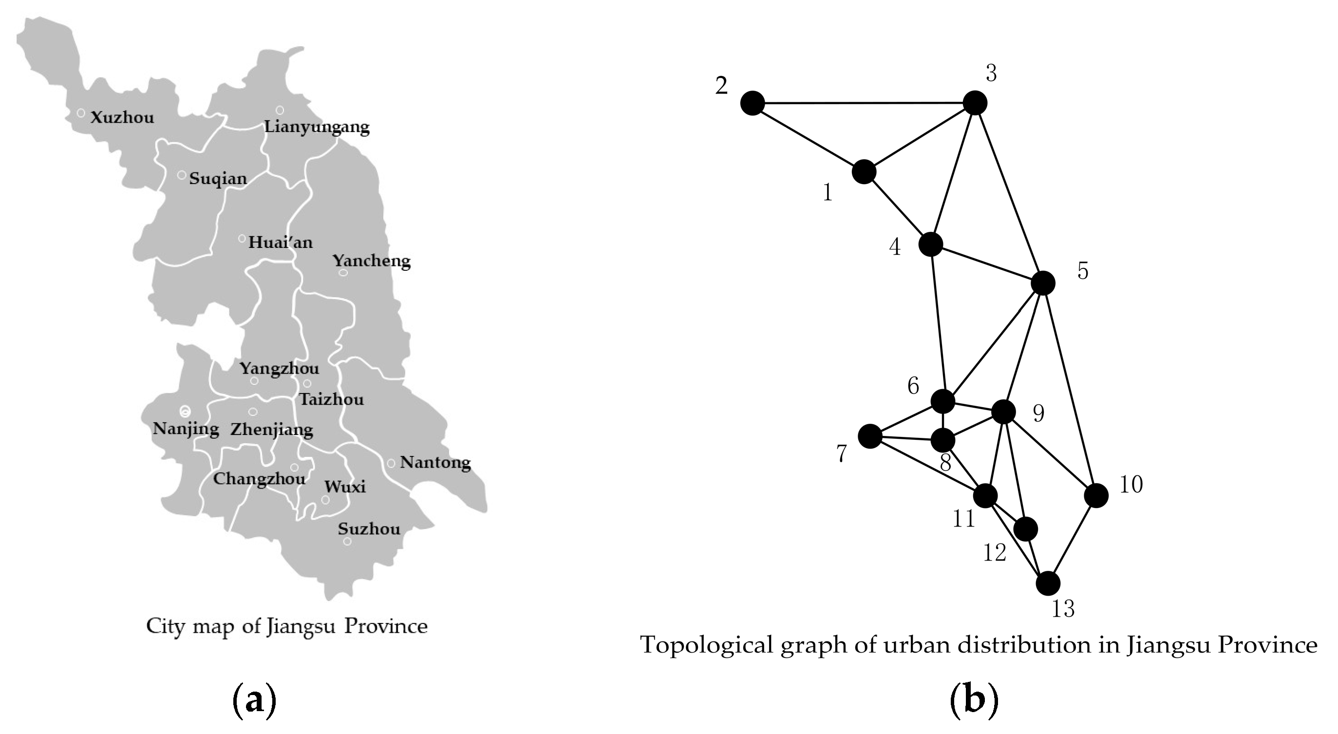
In our study, the GCN network model is built by taking Jiangsu Province as an example. According to whether the 13 prefecture-level cities are directly connected geographically, we determine whether there is an adjacency relationship between the two cities.

For convenient descriptions, city names are replaced by numbers. The numbers correspond to the cities shown in

Table 3. Serial number of the city.

Number	City	Number	City
1	Suqian	8	Zhenjiang
2	Xuzhou	9	Taizhou
3	Lianyungang	10	Nantong
4	Huai’an	11	Changzhou
5	Yancheng	12	Wuxi
6	Yangzhou	13	Suzhou
7	Nanjing

. As shown in Figure 2a, Nanjing is adjacent to Zhenjiang and Changzhou, and not adjacent to Nantong. The adjacency network of each city in Jiangsu Province is extracted and depicted, as shown in Figure 2b.

According to Figure 2b, an adjacency relationship matrix is established based on whether the 13 cities in Jiangsu Province are adjacent in terms of geographical location. Among them, 1 means that two cities are adjacent, which will be taken into account when updating the meteorological factor data in each round; 0 means that two cities are not adjacent or are the same, which will not be taken into account when updating the data in each round. As a result, an adjacency matrix A can be constructed, as shown in

Table 4. Adjacency matrix of cities in Jiangsu Province.

Number	1	2	3	4	5	6	7	8	9	10	11	12	13
1	0	1	1	1	0	0	0	0	0	0	0	0	0
2	1	0	1	0	0	0	0	0	0	0	0	0	0
3	1	1	0	1	1	0	0	0	0	0	0	0	0
4	1	0	1	0	1	1	0	0	0	0	0	0	0
5	0	0	1	1	0	1	0	0	1	1	0	0	0
6	0	0	0	1	1	0	1	1	1	0	0	0	0
7	0	0	0	0	0	1	0	1	0	0	1	0	0
8	0	0	0	0	0	1	1	0	1	0	1	0	0
9	0	0	0	0	1	1	0	1	0	1	1	1	0
10	0	0	0	0	1	0	0	0	1	0	0	0	1
11	0	0	0	0	0	0	1	1	1	0	0	1	1
12	0	0	0	0	0	0	0	0	1	0	1	0	1
13	0	0	0	0	0	0	0	0	0	1	1	1	0

.

The degree matrix D is constructed as shown in

Table 5. Degree matrix of the cities in Jiangsu Province.

Number	1	2	3	4	5	6	7	8	9	10	11	12	13
1	3	0	0	0	0	0	0	0	0	0	0	0	0
2	0	2	0	0	0	0	0	0	0	0	0	0	0
3	0	0	4	0	0	0	0	0	0	0	0	0	0
4	0	0	0	4	0	0	0	0	0	0	0	0	0
5	0	0	0	0	5	0	0	0	0	0	0	0	0
6	0	0	0	0	0	5	0	0	0	0	0	0	0
7	0	0	0	0	0	0	3	0	0	0	0	0	0
8	0	0	0	0	0	0	0	6	0	0	0	0	0
9	0	0	0	0	0	0	0	0	6	0	0	0	0
10	0	0	0	0	0	0	0	0	0	3	0	0	0
11	0	0	0	0	0	0	0	0	0	0	5	0	0
12	0	0	0	0	0	0	0	0	0	0	0	3	0
13	0	0	0	0	0	0	0	0	0	0	0	0	3

:

According to the data provided by the “Table of Observation Data for Basic Meteorological Elements of China’s Surface Meteorological Stations” [21], the observation station data of 13 prefecture-level cities of Jiangsu Province were selected in our experiments. The station number, station name, latitude, longitude, altitude of the pressure sensor, and altitude of the observation site are shown in

Table 6. Observation data of basic meteorological elements at ground meteorological stations in Jiangsu Province.

Province	District Station Number	Station Name	Latitude (d m)	Longitude (d m)	Altitude of the Barometric Sensor (m)	Altitude of the Observation Site (m)
Jiangsu	58238	Nanjing	3156	11,854	36.4	35.2
Jiangsu	58354	Wuxi	3137	12,021	4.1	3.2
Jiangsu	58027	Xuzhou	3417	11,709	42.0	41.2
Jiangsu	58342	Changzhou	3143	11,933	7.7	6.9
Jiangsu	58349	Suzhou	3125	12,034	8.9	8.0
Jiangsu	58259	Nantong	3205	12,059	4.6	4.8
Jiangsu	58044	Lianyungang	3432	11,914	4.7	4.7
Jiangsu	58141	Huai’an	3338	11,856	13.7	12.5
Jiangsu	58154	Yancheng	3326	12,012	6.8	2.5
Jiangsu	58245	Yangzhou	3225	11,925	14.7	9.9
Jiangsu	58341	Zhenjiang	3159	11,936	10.2	6.6
Jiangsu	58246	Taizhou	3233	12,000	3.4	2.6
Jiangsu	58131	Suqian	3358	11,813	26.0	25.0

.

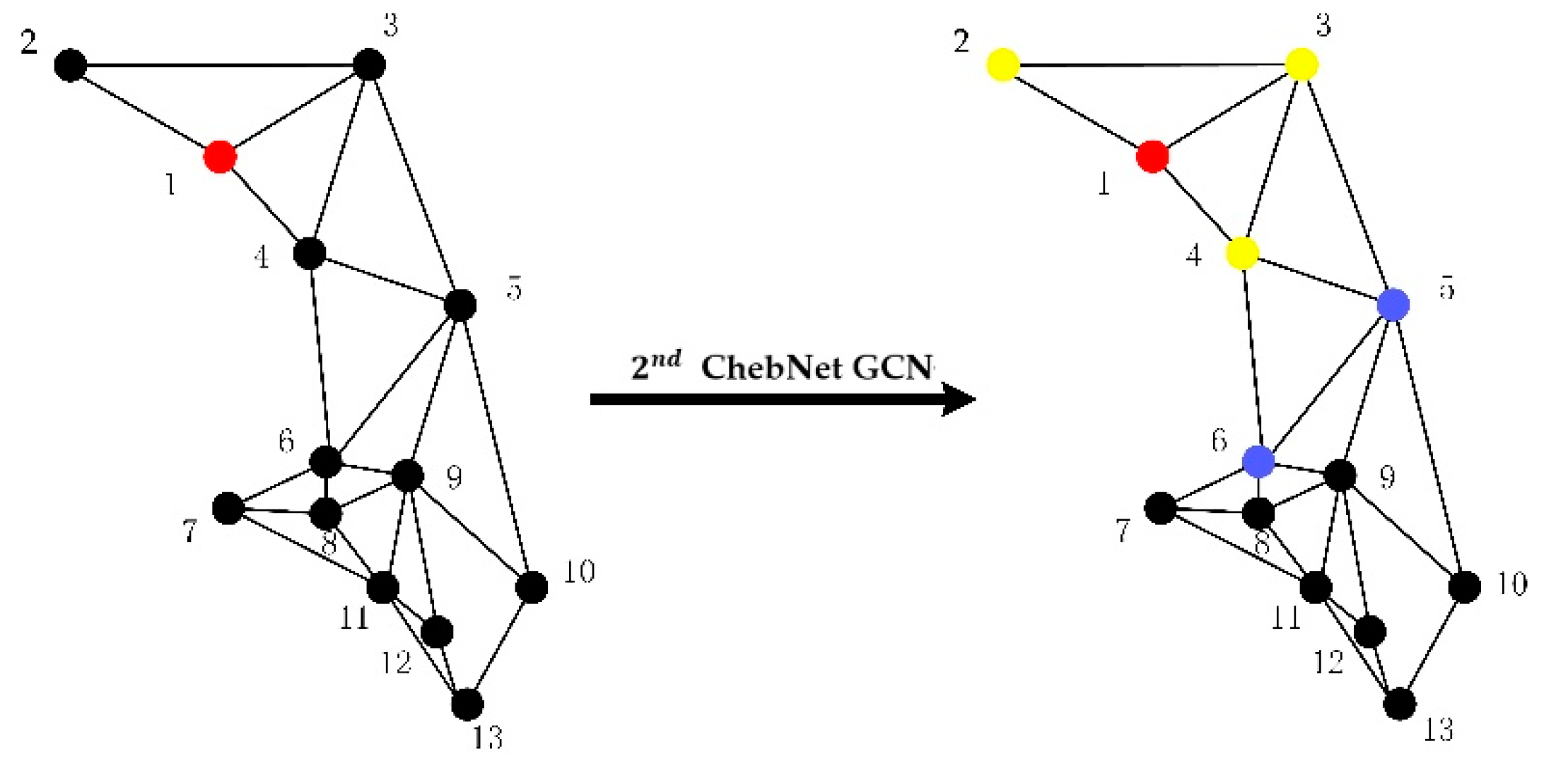
For meteorological data with a graph structure, the spatial-temporal correlation in the meteorological data is extracted using graph convolution, that is, the correlations between the meteorological data of the surrounding sites and the temperature data of the target sites. As shown in Figure 3, with node 1 as the starting point of the GCN convolution operation, the meteorological information of adjacent nodes 2, 3, and 4, which are directly connected to node 1, can be extracted using first-order ChebNet graph convolution. Then, after the updated data are processed by the activation function, we perform the first-order ChebNet graph convolution again to extract the meteorological information of nodes 5 and 6, which are directly connected to nodes 2, 3, and 4. Nodes 2, 3, and 4 can be considered as first-order adjacent nodes centered on node 1, and nodes 5 and 6 can be regarded as second-order adjacent nodes centered on node 1.

Using the second-order ChebNet graph convolution, the convolution kernel can directly extract information about the surrounding first-order neighboring nodes 2, 3, 4, and second-order neighboring nodes 5, 6 centered on node 1. The detailed implementation process of the second-order ChebNet graph convolution is shown in Figure 4.

Generally, high-order convolution nodes can be achieved by convoluting and stacking multiple low-order nodes. For example, a second-order convolution can be accumulated by two first-order convolutions. When the order is 0, each node can only extract its meteorological features but cannot extract the meteorological features of surrounding nodes. However, the higher the order is not better. When the order is too large, the complexity of the network and the computation time will increase obviously. Taking the graph network of Jiangsu Province as an example, with node 1 as the starting point, the meteorological information of each node in the province can be extracted by 4 times the convolution and superposition of first-order nodes. In this research, it is not necessary to extract the features of all nodes in the research area. According to the experimental verification, the first-order GCN graph convolution operations are performed twice in this research.

3.2.2. BiLSTM Model

LSTM solves the long-term dependency problem of RNN and performs well in processing time series with a long time span. However, the transmission of the unit state in LSTM is unidirectional from front to back [24], so the LSTM model can only learn the meteorological features of past moments and cannot learn the meteorological features of future moments. BiLSTM means bidirectional LSTM, which means that the signal propagates backward and forward in time [25]. The BiLSTM can learn the features of future meteorological information while using past meteorological information and apply recursion and feedback to it. Its prediction results are more accurate than unidirectional LSTM [26].

The LSTM network unit comprises a cell, an input gate, an output gate, and a forget gate. The state unit is employed to coordinate the operation of the whole network. The calculation formula of the LSTM network unit implemented by gating is as follows:

$$f_t=\sigma \left(W_f{x}_t+U_f{h}_{t-1}+b_f\right)$$

(2)

$$i_t=\sigma \left(W_i{x}_t+U_i{h}_{t-1}+b_i\right)$$

(3)

$${\tilde{C}}_t=\tanh \left(W_c{x}_t+U_c{h}_{t-1}+b_c\right)$$

(4)

$$C_t=C_{t-1}\cdot f_t+{\tilde{C}}_t\cdot i_t$$

(5)

$$o_t=\sigma \left(W_o{x}_t+U_o{h}_{t-1}+b_o\right)$$

(6)

$${\mathrm{h}}_{\mathrm{t}}=o_{\mathrm{t}}\cdot \tanh \left({\mathrm{c}}_{\mathrm{t}}\right)$$

(7)

Here, $f_t$ is the forget gate. $i_t$ is the input gate and $o_t$ is the output gate. $C_t$ is the internal state at time t. $W$, $U$, and $b$ are the model parameters.

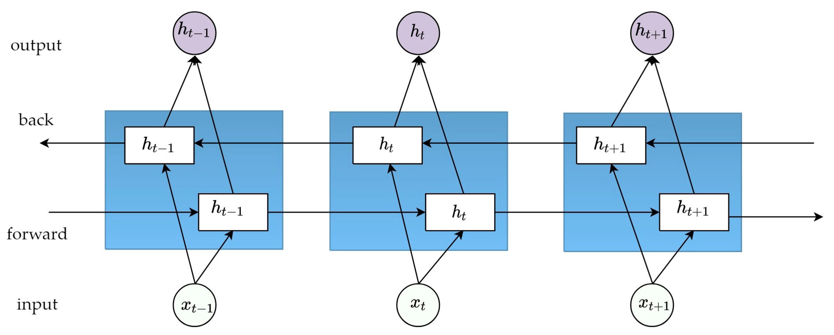
The structure of the BiLSTM network is shown in Figure 5. The BiLSTM network is a bidirectional structure that makes the input flow in both directions to preserve future and past information. Therefore, BiLSTM-based models can better mine the association features of time series data.

Suppose that $\overrightarrow{h_{\mathrm{t}}}$ is the hidden layer state of the forward LSTM network at time $t$, and its calculation formula is as described in Equation (8).

$$\overrightarrow{h_t}=\mathrm{LSTM}\left(x_t,{\overrightarrow{h}}_{t-1}\right)$$

(8)

where $x_t$ is the input at time $t$ and ${\overrightarrow{h}}_{t-1}$ is the hidden layer state of the forward LSTM network at time $t-1$. $h_t$ is the hidden layer state of the back LSTM network at time $t$, and its calculation formula is as shown in Equation (9):

$$\overleftarrow{h_t}=\mathrm{LSTM}\left(x_t,{\overleftarrow{h}}_{t-1}\right)$$

(9)

where $x_t$ is the input at time $t$, and ${\overleftarrow{h}}_{t-1}$ is the hidden layer state of the back LSTM network at time $t-1$. The output of the BiLSTM network is the combination of two hidden layer states $\overrightarrow{h_t}$ and $\overleftarrow{h_t}$, to form the whole hidden state $h_t$ of the network.

3.2.3. GCN-BiLSTM Model

After preprocessing the original meteorological time series data, such as data cleaning and standardization, the data set is divided into training sets, validation sets, and test sets. After the initial data pass through the two-layer GCN network, the feature extraction of meteorological information from the surrounding area is achieved. After this, the information contains spatial features. The output of the previous layer is further fed into the BiLSTM network. Then, the final output $\{y_1,y_2,\dots y_n\}$is obtained after dropout optimization and 6 fully connected layers. When the input data is the training set, the output values $\{y_1,y_2,\dots y_n\}$and the actual temperature $\{T_1,T_2,\dots ,T_n\}$ are used to calculate the loss of mean squared error. The model is continuously optimized by the Adam optimizer. When the input data are the test set, no loss calculation and model optimization are performed, and the output values are the predicted temperature values of the GCN-BiLSTM model. The detailed workflow of the GCN-BiLSTM model is shown in Figure 6.

4. Results and Discussion

4.1. Experimental Data

The experimental data in this research are the daily weather data of 2071 stations in the Chinese mainland for a total of 3531 days between 1 May 2010, and 31 December 2019. After the gray correlation analysis, eight attributes with correlations greater than 0.88 were selected, including average temperature, average humidity, sunshine duration, precipitation, average wind speed, maximum temperature, average pressure, and date. After data processing by the time sliding window, 3521 experimental data are retained for each site. The data sets are divided into the training set, validation set, and test set according to the ratio of 8:1:1. To analyze the performance of each model, the data sets will be re-divided according to different experiments, and the model will be retrained to perform prediction experiments.

4.2. Baseline Models

In this research, to evaluate the performance of the proposed GCN-BiLSTM model, we select three typical models for controlled experiments. Autoregressive Integrated Moving Average (ARIMA) [27] belongs to the classical mathematical statistics method, which is good at dealing with temperature data with prominent non-stationary fluctuation characteristics. LSTM [15] is a commonly used model in time series processing research. It can learn the temporal dependence of temperature from historical data and has good performance in handling data with time series features. The Deep Feedforward Network (DFN) [28] is a DL method that can learn the relationships between meteorological elements and temperature to perform accurate predictions.

ARIMA: This model converts a nonstationary time series into a stationary time series, and then regresses the lag values of the dependent variables, the present values, and lag values of the random errors to deal with time series forecasting problems.

LSTM: The model explores the dependencies between sequence elements by transferring internal states. The gating mechanism is applied to solve the defect of the RNN gradient update.

DFN: DFN consists of an input layer, an output layer, and multiple hidden layers. There is no backward feedback in the network, and the signal propagates unidirectionally from the input layer to the output layer.

4.3. Evaluation Metrics

In this research, the root mean squared error (RMSE) and mean absolute error (MAE) are employed as evaluation metrics to measure model performance and analyze prediction accuracy. The RMSE and MAE values can be considered the absolute Celsius error between the true and predicted values. The calculation formula is described as follows.

$$RMSE=\sqrt{\frac{1}{N}{\displaystyle \sum }_{i=1}^N{\left(y_i^{\prime }-y_i\right)}^2}$$

(10)

$$MAE=\frac{1}{N}{\displaystyle \sum }_{i=1}^N\left|y_i^{\prime }-y_i\right|$$

(11)

Here, $y_i^{\prime }$ is the predicted value. $y_i$ is the actual value. $N$ is the sample number of the test set. Smaller RMSE and MAE indicate higher prediction accuracy of the model; conversely, higher evaluation metrics indicate lower prediction accuracy.

4.4. Results

4.4.1. 14-Day Temperature Prediction Experiment

To evaluate the performance of the model for short-term temperature prediction and the prediction performance differences among each model, the temperature prediction experiments are set up for the next 14 days, as follows in this research. We took Nanjing city as the research area and set the number of time-sliding windows to 30. The number of input nodes is 30 × 8, a total of 240, and the number of output forecast days is 14 days. We use training and validation datasets to train GCN-BiLSTM, DFN, and LSTM, respectively. Then, three baseline models and GCN-BiLSTM are employed to forecast 14-day temperatures by selecting 10 random time points. The RMSE and MAE of each model are calculated by taking the average results of 10 experiments.

The experimental results of temperature prediction for the next 14 days are shown in

Table 7. Experimental results of temperature prediction for the next 14 days.

Forecast Days	RMSE/°C				MAE/°C
	GCN-BiLSTM	DFN	LSTM	ARIMA	GCN-BiLSTM	DFN	LSTM	ARIMA
1	1.534	2.933	2.245	2.124	2.414	3.445	2.982	4.122
2	1.459	3.238	2.357	2.245	2.358	3.562	3.152	4.258
3	1.745	3.596	2.458	2.458	2.574	3.421	2.863	4.022
4	1.862	3.895	2.534	3.518	2.682	3.832	3.450	4.249
5	2.273	4.156	2.898	4.056	2.799	3.751	3.715	4.348
6	2.479	3.780	3.487	4.585	3.171	4.141	3.887	4.985
7	2.635	4.286	3.911	5.287	2.854	4.358	3.956	5.681
8	2.956	4.342	3.678	4.928	2.963	4.655	3.658	5.852
9	2.831	4.756	3.756	5.580	3.192	4.855	4.254	6.258
10	3.149	4.856	3.895	5.787	3.487	4.956	4.058	6.574
11	3.455	4.560	4.355	6.456	3.223	5.412	4.535	7.152
12	3.624	4.981	4.259	6.854	3.594	5.758	4.914	6.895
13	3.368	5.415	4.560	7.758	3.261	6.182	5.112	7.556
14	4.023	5.676	4.457	8.236	3.758	5.962	5.457	8.457
Average	2.671	4.319	3.489	4.991	3.024	4.592	4.010	5.744

.

4.4.2. Multi-Regional Temperature Prediction Experiment

Temperature prediction experiments are conducted in several cities to evaluate the performance differences of each model for temperature prediction in different regions. Harbin, Beijing, Jinan, Qingdao, Nanjing, Hangzhou, Guangzhou, and Shenzhen are selected as the experimental cities. The number of time-sliding windows is set to 30. The number of input nodes is 30 × 8 for a total of 240, and the number of output forecast days is 1 day.

The experimental RMSE and MAE of temperature prediction for the next day at 8 cities are shown in

Table 8. Comparison of RMSE for multiregional temperature prediction.

City	GCN-BiLSTM	DFN	LSTM	ARIMA
Harbin	2.294	3.546	2.849	2.868
Beijing	2.035	3.324	2.751	3.146
Jinan	2.337	3.660	2.955	2.886
Qingdao	1.848	2.915	2.467	2.748
Nanjing	2.141	3.223	2.711	2.755
Hangzhou	1.601	2.882	2.445	2.668
Guangzhou	1.485	2.664	2.212	2.524
Shenzhen	1.510	2.672	2.313	2.329
average	1.906	3.111	2.588	2.741

and

Table 9. Comparison of MAE for multiregional temperature prediction.

City	GCN-BiLSTM	DFN	LSTM	ARIMA
Harbin	2.880	3.857	3.462	4.402
Beijing	2.765	3.714	3.351	4.246
Jinan	2.886	3.970	3.551	4.583
Qingdao	2.372	3.446	2.821	4.057
Nanjing	2.612	3.582	2.928	4.356
Hangzhou	2.487	3.233	2.785	4.012
Guangzhou	2.345	3.120	2.694	3.924
Shenzhen	2.318	3.335	2.743	3.846
average	2.583	3.532	3.042	4.178

, respectively.

4.5. Discussion

From the 14-day temperature prediction experiments, it can be seen in Table 6 that for the average RMSE and MAE of the temperature forecast for the next 14 days, the GCN-BiLSTM model reaches 2.671 °C and 3.024 °C, respectively. Compared to LSTM, DFN, and ARIMA models, the RMSE value decreased by 23.45%, 38.16%, and 46.48%; the MAE value decreased by 32.61%, 34.15%, and 47.35%, respectively.

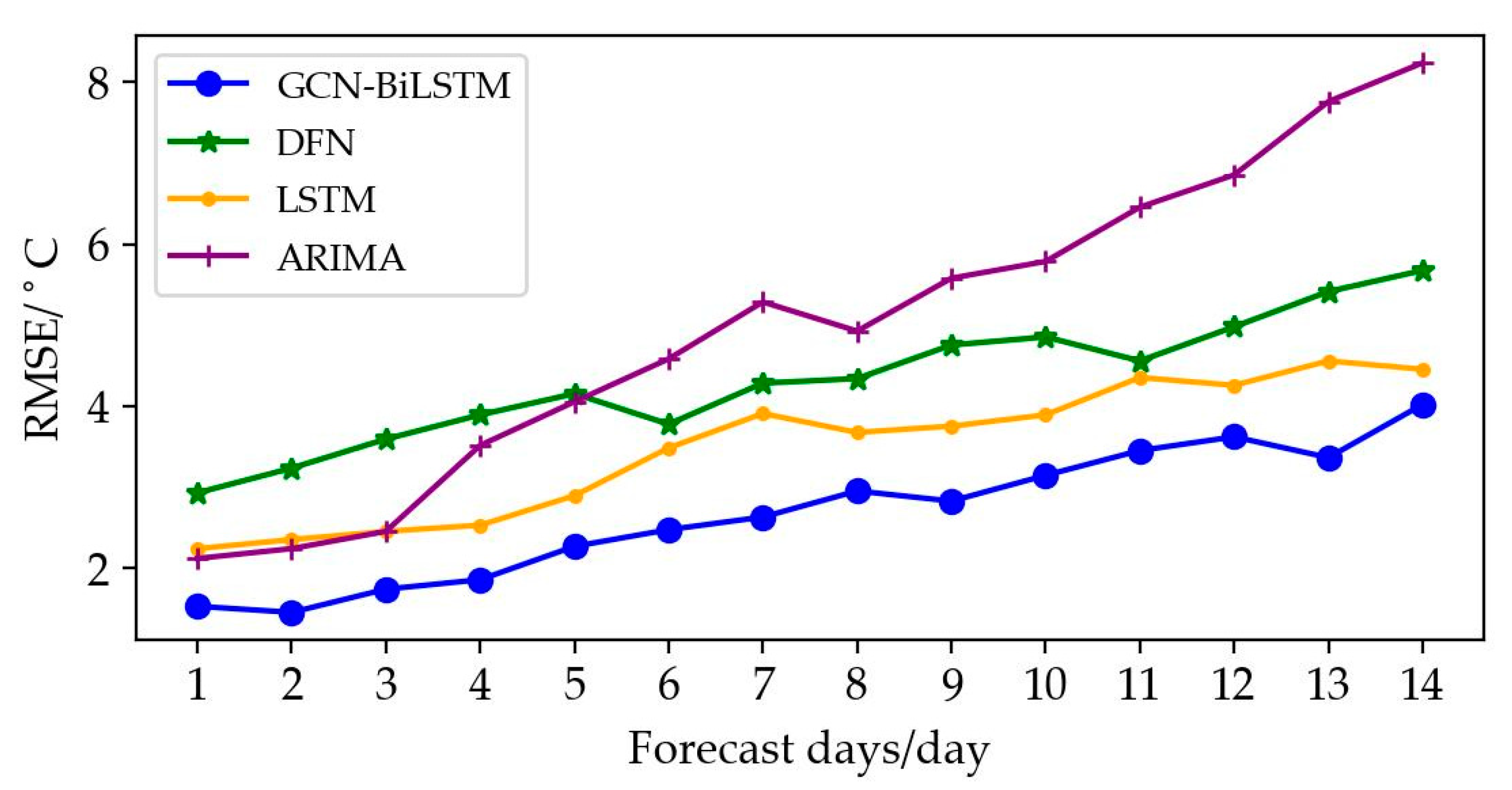
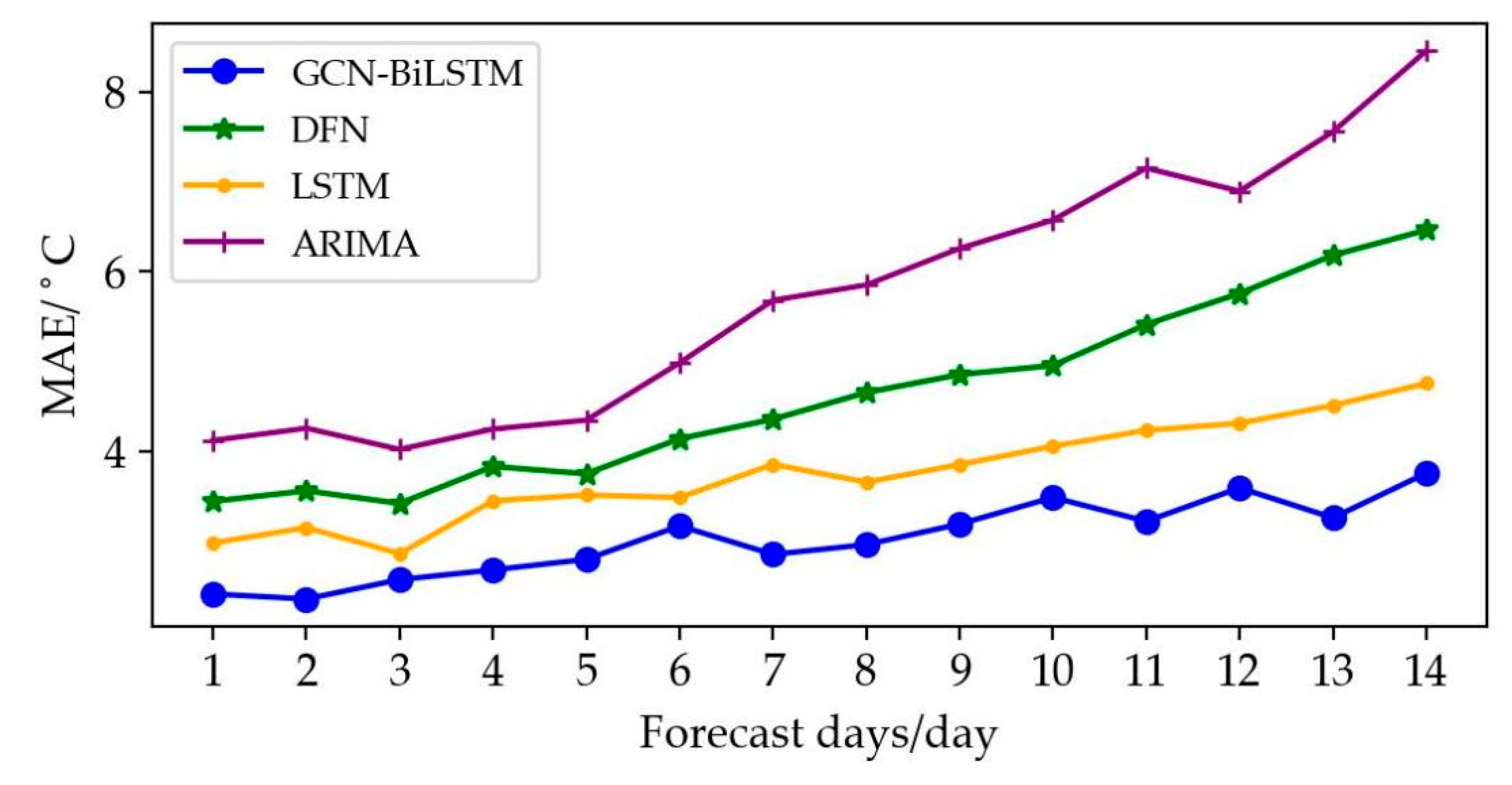
The RMSE and MAE variations of the four models are shown in Figure 7 and Figure 8. It can be seen that the GCN-BiLSTM model achieves the best prediction performance for different predictions in different experimental regions. Specifically, as the number of forecast days increases, both the RMSE and MAE errors of these models appear to have an increasing trend. The ARIMA model outperforms the DFN and LSTM methods in terms of RMSE for short forecast days. However, due to its limitation of single attribute prediction, ARIMA performs poorly in longer time-step prediction. As shown in Figure 7, the ARIMA error exceeds the DFN, with the highest error from day 5, and the error tends to increase significantly afterward. This indicates that the DFN model and the GCN-BiLSTM model, which integrate multiple influencing factors, have better performance than the ARIMA model, which only considers single factors. After the 7th day, the RMSE and MAE of the DFN model continue to get higher. This is because the DFN model does not analyze the time-series features of temperature data and performs poorly in long-term temperature prediction. From the 7th day to the 14th day, the LSTM model and the GCN-BiLSTM model, which take into account the time series features, show better performance in long-term temperature prediction. Their RMSE and MAE are relatively lower, and the change in errors is smaller. Further, compared with the LSTM model, which only considers temporal features, the average RMSE and MAE of GCN-BiLSTM decrease by 23.45% and 32.61%, respectively, in the long-short term predictions. This demonstrates that the GCN-BiLSTM model, considering spatial-temporal features, has better prediction performance. This is because it captures the influence of meteorological factors of the surrounding area on the target area from the perspective of urban spatial distribution. Meanwhile, the information containing spatial features is also modeled based on temporal features, and a DL model with spatial-temporal feature capture capability is constructed. Overall, the GCN-BiLSTM model performed better in the learning of temporal and spatial features., and has the best performance in long-short term temperature forecasting.

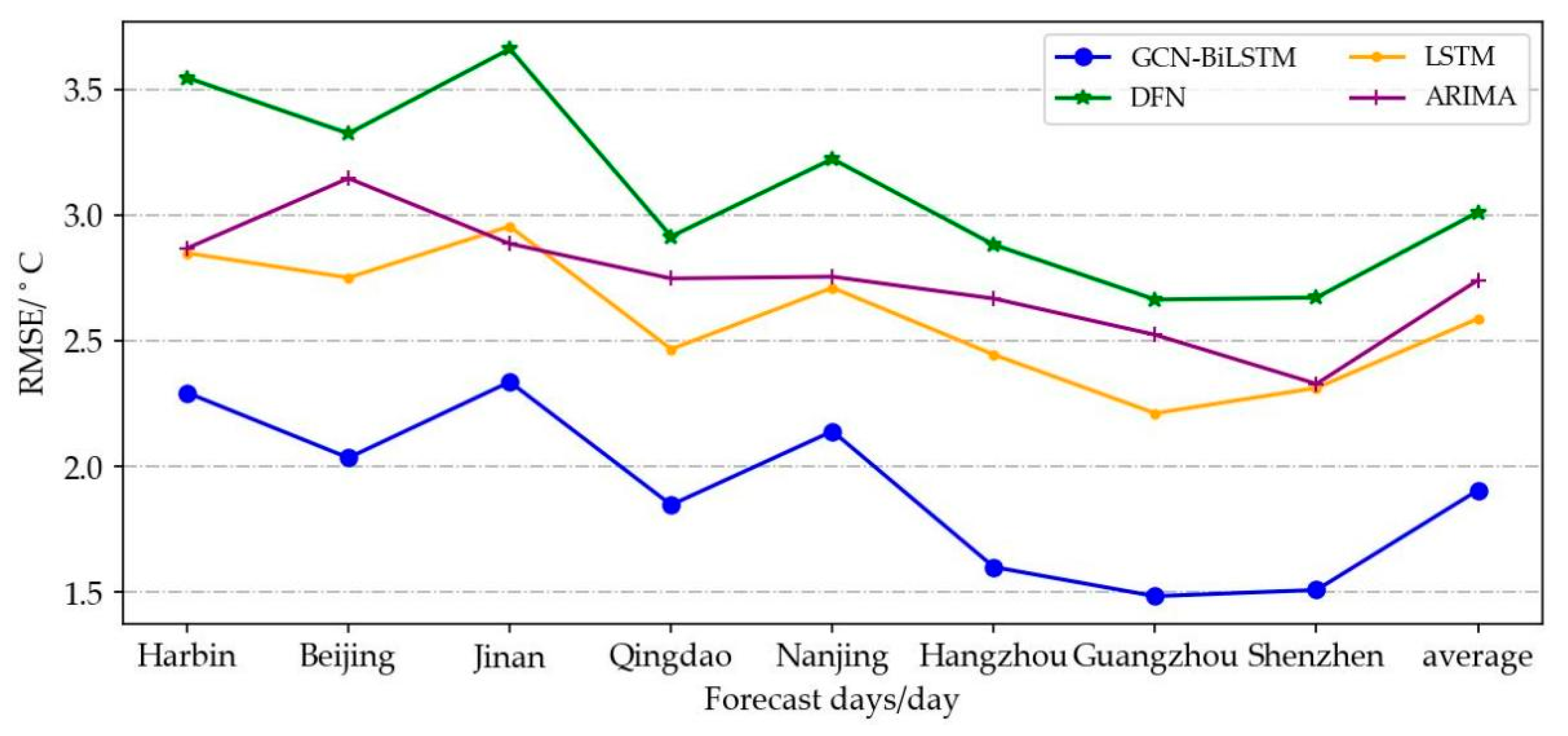
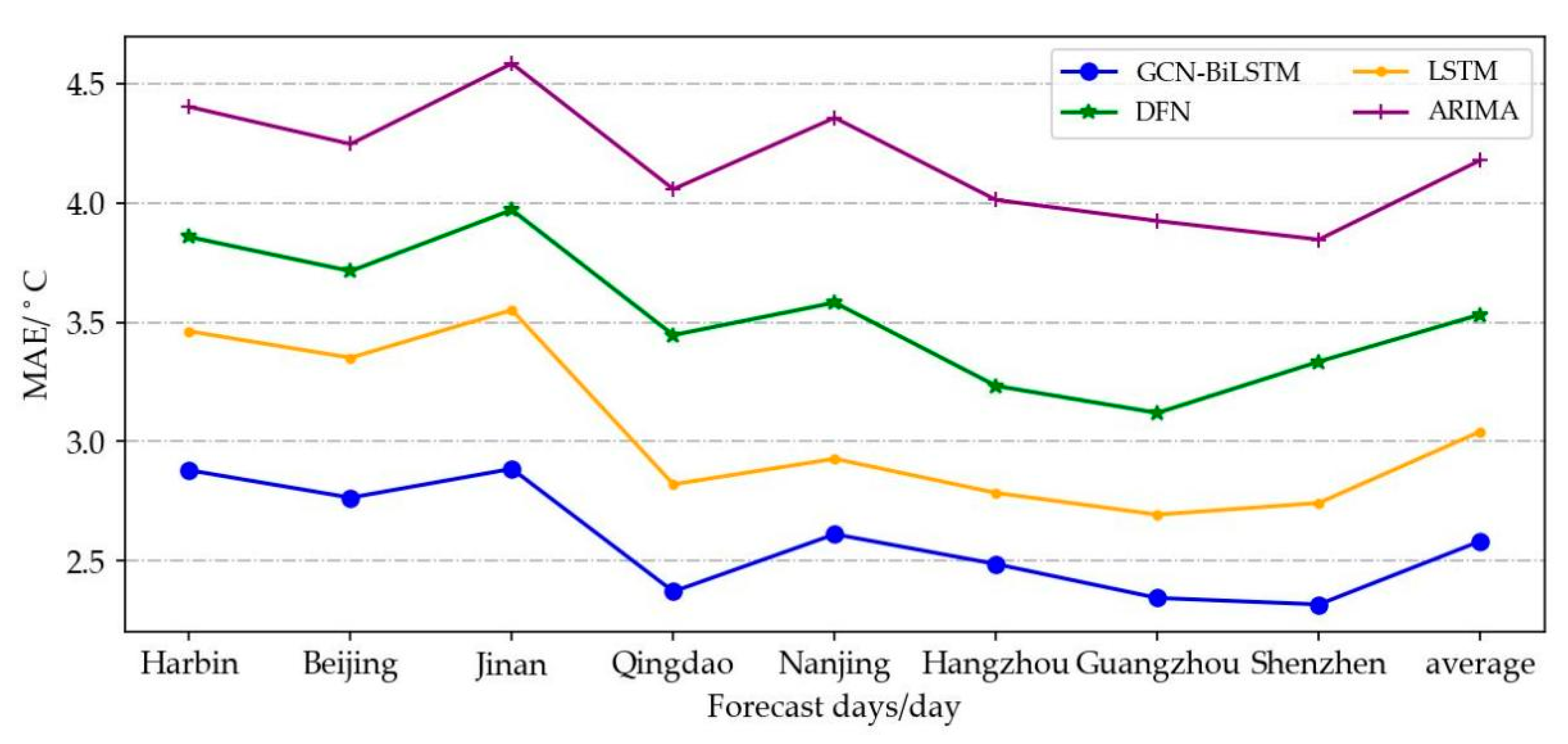
From the multi-regional temperature prediction experiments, as shown in Table 8, the average RMSE of the GCN-BiLSTM model is 1.906 °C, which is 26.35%, 33.79%, and 38.73% lower than that of the LSTM, ARIMA, and DFN models, respectively. Similarly, in terms of absolute error, the average MAE of the GCN-BiLSTM model is 2.583 °C, which is 15.09%, 26.87%, and 38.18% lower than that of LSTM, DFN, and ARIMA, respectively, as shown in Table 9.

The RMSE and MAE of different models in different cities are shown in Figure 9 and Figure 10. As can be seen in Figure 9, the GCN-BiLSTM model outperforms ARIMA, LSTM, and DFN in temperature prediction in different regions. As in the above analysis, the ARIMA model outperforms the DFN model in terms of RMSE in all research cities. However, for MAE, the result is the opposite. The LSTM model still performs better than the ARIMA model and the DFN model. Comprehensively, the prediction accuracy of the four models has a similar trend, but the GCN-BiLSTM model is more adaptive in each region. This is because the GCN-BiLSTM model can capture the spatial-temporal features of the temperature data in the current region. Specifically, the RMSE of the GCN-BiLSTM model in Hangzhou, Qingdao, Guangzhou, and Shenzhen are lower than the average of the eight cities, while the RMSE in Harbin, Beijing, Jinan, and Nanjing are higher than the average. The GCN-BiLSTM model has the optimal performance for temperature prediction in Guangzhou, with an RMSE of 1.485 °C, which is 22.09% lower than the average. The worst performance for Jinan is 2.337 °C, which is 22.61% higher than the average. As shown in Figure 10, in terms of MAE, the GCN-BiLSTM model performs best for temperature prediction in Guangzhou. In Jinan and Harbin, the MAE is high, and the GCN-BiLSTM model performs well.

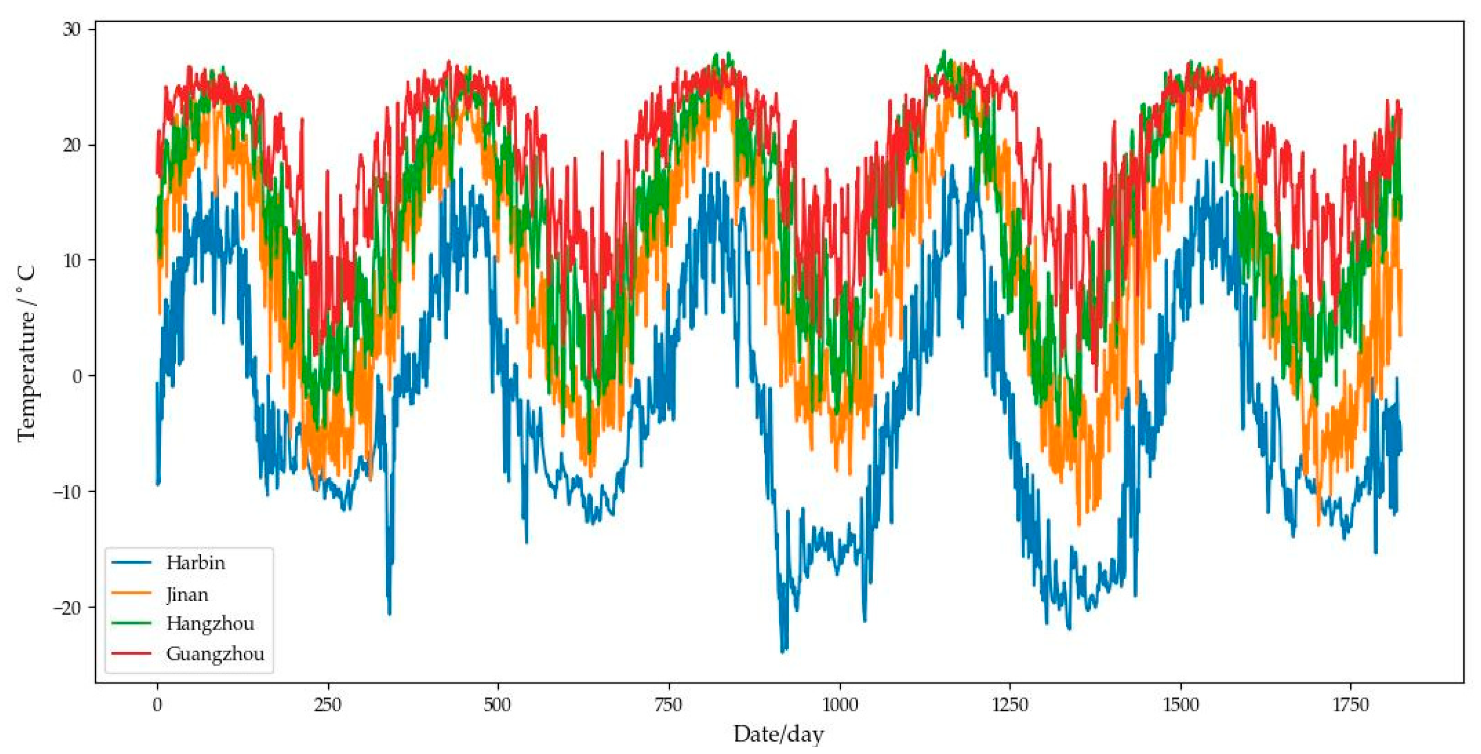
Figure 11 depicts the temperature trends in the four cities of Harbin, Jinan, Hangzhou, and Guangzhou during the five-year period from 1 May 2014 to 1 May 2019. As shown in Figure 11, the temperature difference in Guangzhou is small throughout the year, about 24 °C to 26 °C due to its low latitude, its proximity to the South China Sea, and its subtropical maritime climate. Therefore, the prediction accuracy in Guangzhou is better than in other cities. However, in Harbin and Jinan, the temperature fluctuates throughout the year, with a temperature difference of about 35 °C. The prediction accuracy of the model is lower than in other cities, with more slight fluctuations.

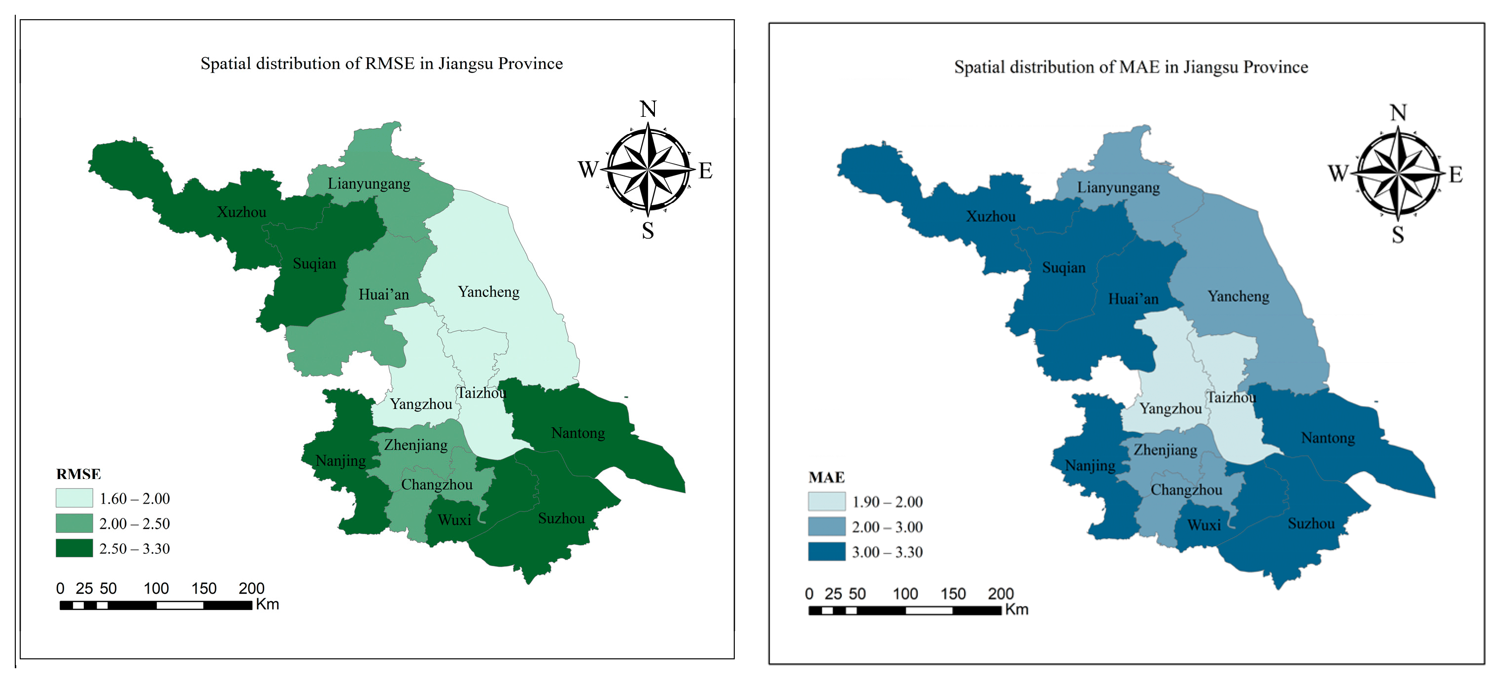
To further explore the spatial correlation of GCN-BiLSTM, the RMSE and MAE of the temperature prediction results for each city in Jiangsu province are spatially visualized, as shown in Figure 12. Hereinto, the average values of RMSE and MAE for the 14-day temperature prediction results are selected in the figure. Cities located at the edge of the study area and with fewer neighbor nodes (including first-order and second-order nodes) have higher prediction errors, such as Suqian and Xuzhou. Cities with more neighbor nodes have smaller prediction errors, such as Yangzhou and Taizhou. GCN is employed to extract the spatial features of the city’s topological maps in our model. If there are more neighbor nodes in the target region, the more features used to extract spatial correlation, the more accurate the prediction will be. However, when the number of neighbor nodes exceeds a certain threshold, the prediction effect does not improve significantly, such as in Yancheng. We consider that when there are too many neighbor nodes, it will bring additional noisy data to affect feature extraction.

In summary, the GCN-BiLSTM model shows the best performance in temperature prediction among the above four models. The model has significant spatial performance differences and is influenced by the meteorological factors of the surrounding areas. The The GCN-BiLSTM model has higher accuracy in cities with stable temperature fluctuations and slight temperature differences than in cities with sharp temperature fluctuations and significant temperature differences.

5. Conclusions

It is difficult to forecast future weather changes because of the nonlinear characteristics and spatial-temporal heterogeneity of meteorological time-series data. For accurate and effective temperature prediction, GCN and BiLSTM were integrated to construct the GCN-BiLSTM temperature prediction model in this research. Then, the influence of multiple meteorological elements and time-sliding windows on the forecast results was analyzed and compared among the four models.

By analyzing the influence of multiple meteorological elements and time-sliding windows on the forecast results and the forecast performance of each temperature forecast model on meteorological time series from different time and space perspectives, this research draws the following conclusions.

(1) Multidimensional meteorological features were used to replace single meteorological features in the GCN-BiLSTM model. The sliding time window setting was added to extend the model input data dimension and enable the model to further learn the correlation of multidimensional meteorological elements and temporal characteristics of historical meteorological data on future temperatures and improve prediction accuracy.

(2) Compared to baseline DL models, the prediction effect of the GCN-BiLSTM model was significantly improved, benefiting from the time series and spatial features of the meteorological data. GCN-BiLSTM model had the lowest RMSE and MAE values, which can accurately predict the future temperature with ±2 °C average errors.

(3) From the perspective of forecast time, the prediction accuracy of each model decreases as the number of prediction days increases. Among them, the error curve of the GCN-BiLSTM-based prediction is relatively smooth. From the perspective of space, the prediction effect of the GCN-BiLSTM model is influenced by the meteorological factors of neighboring regions. The prediction results of each model in areas with smaller annual temperature differences are better than those with larger annual temperature differences.

In the future, we plan to enhance this research in the following ways. First, this research makes model performance comparisons for temperature prediction in different regions and analyzes the spatial performance differences of the models. Most of China’s areas are located in the temperate monsoon climate zone, the subtropical monsoon climate zone, and the temperate continental climate zone, with noticeable seasonal changes. In future research, the performance differences of the model will be considered in different seasons. In addition, controlled experiments can be conducted and analyzed on season or month scales. Second, only adjacency is considered a spatial feature for constructing the experimental graph network in this research, in which the spatial feature relationship is relatively simple. Furthermore, in this research, the station temperature is used to represent the temperature of the city where the station is located, which should be further optimized on a smaller scale. For example, we can generate large amounts of raster data to describe the spatial feature relationship of meteorological time series by further interpolation methods from points to surfaces.

References

1. Dyurgerov, M. Mountain and subpolar glaciers show an increase in sensitivity to climate warming and intensification of the water cycle. J. Hydrol. 2003, 282, 164–176. [Google Scholar] [CrossRef]
2. WMO. Reducing and managing risks of disasters in a changing climate. WMO Bull. 2013, 62, 23–31. [Google Scholar]
3. He, Y.; Zhang, Z.; Theakstone, W.H.; Chen, T.; Yao, T.; Pang, H. Changing features of the climate and glaciers in China’s monsoonal temperate glacier region. J. Geophys. Res.-Atmos. 2003, 108. [Google Scholar] [CrossRef]
4. Tao, S.Y.; Zhao, S.X.; Zhou, X.P.; Ji, L.R.; Sun, S.Q.; Gao, S.T.; Zhang, Q.Y. Advances in weather science and weather forecasting. Atmos. Sci. 2003, 27, 451–467. [Google Scholar]
5. Gustavo, Z.; Nuria, P.G.; Francisco, A.; Valdir, A.S.; Charlei, A. A Short Critical History on the Development of Meteorology and Climatology. Climate 2017, 5, 23. [Google Scholar]
6. Bogdanovs, N.; Bistrovs, V.; Petersons, E.; Ipatovs, A.; Belinskis, R. Weather prediction algorithm based on historical data using kalman filter. In Proceedings of the 2018 Advances in Wireless and Optical Communications (RTUWO), Riga, Latvia, 15–16 November 2018; pp. 94–99. [Google Scholar]
7. Pérez-Vega, A.; Travieso, M.C.; Hernández-Travieso, G.J.; Alonso, B.J.; Dutta, K.M.; Singh, A. Forecast of temperature using support vector machines. In Proceedings of the 2016 International Conference on Computing, Communication and Automation (ICCCA), Greater Noida, India, 29–30 April 2016; IEEE: New York, NY, USA, 2016; pp. 388–392. [Google Scholar]
8. Liang, S.; Wang, D.; Wu, J.; Wang, R.; Wang, R. Method of Bidirectional LSTM Modelling for the Atmospheric Temperature. Intell. Autom. Soft Comput. 2021, 30, 701–714. [Google Scholar] [CrossRef]
9. Federico, C.; Massimiliano, B. Wind speed and wind energy forecast through Kalman filtering of Numerical Weather Prediction model output. Appl. Energy 2012, 99, 154–166. [Google Scholar]
10. Wang, H.; Huang, J.; Zhou, H.; Zhao, L.; Yuan, Y. An integrated variational mode decomposition and ARIMA model to forecast air temperature. Sustainability 2019, 11, 4018. [Google Scholar] [CrossRef] [Green Version]
11. Kisi, O.; Cimen, M. Precipitation forecasting by using wavelet-support vector machine conjunction model. Eng. Appl. Artif. Intell. 2012, 25, 783–792. [Google Scholar] [CrossRef]
12. Radhika, Y.; Shashi, M. Atmospheric temperature prediction using support vector machines. Int. J. Comput. Theory Eng. 2009, 1, 55. [Google Scholar] [CrossRef] [Green Version]
13. Venkadesh, S.; Hoogenboom, G.; Potter, W.; McClendon, R. A genetic algorithm to refine input data selection for air temperature prediction using artificial neural networks. Appl. Soft Comput. 2013, 13, 2253–2260. [Google Scholar] [CrossRef]
14. Abbot, J.; Marohasy, J. The application of machine learning for evaluating anthropogenic versus natural climate change. GeoResJ 2017, 14, 36–46. [Google Scholar] [CrossRef]
15. Feng, H.C.; Xu, D.G. LSTM-based weather temperature prediction. Digit. Des. 2018, 7, 52. [Google Scholar]
16. Wu, Y.; Wang, X. PM2. 5 concentration prediction using improved LSTM in big data environment. Fresenius Environ. Bull. 2020, 29, 10098–10108. [Google Scholar]
17. Qiao, B.; Wu, Z.; Tang, Z.; Wu, G. Sea surface temperature prediction approach based on 3D CNN and LSTM with attention mechanism. In Proceedings of the 2022 24th International Conference on Advanced Communication Technology (ICACT), PyeongChang Kwangwoon_Do, Republic of Korea, 13–16 February 2022; IEEE: New York, NY, USA, 2022; pp. 342–347. [Google Scholar]
18. Jeong, S.; Park, I.; Kim, H.; Song, C.; Kim, H. Temperature prediction based on bidirectional long short-term memory and convolutional neural network combining observed and numerical forecast data. Sensors 2021, 21, 941. [Google Scholar] [CrossRef]
19. Cao, X.; Zhong, Y.; Zhou, Y.; Wang, J.; Zhu, C.; Zhang, W. Interactive temporal recurrent convolution network for traffic prediction in data centers. IEEE Access 2017, 6, 5276–5289. [Google Scholar] [CrossRef]
20. Zhao, L.; Song, Y.; Zhang, C.; Liu, Y.; Wang, P.; Lin, T.; Deng, M.; Li, H. T-gcn: A temporal graph convolutional network for traffic prediction. IEEE Trans. Intell. Transp. Syst. 2019, 21, 3848–3858. [Google Scholar] [CrossRef] [Green Version]
21. Meteorological Information Center. Daily Meteorological Dataset of Basic Meteorological Elements of China National Surface Weather Station (V3.0) (1951–2010); National Tibetan Plateau Data Center: Qinghai, China, 2019; Available online: http://data.cma.cn/ (accessed on 19 November 2022).
22. Zhu, H.; Lin, Y.; Liu, Z.; Fu, J.; Chua, T.-S.; Sun, M. Graph Neural Networks with Generated Parameters for Relation Extraction. arXiv 2019, arXiv:1902.00756. [Google Scholar]
23. Kipf, T.N.; Welling, M. Semi-Supervised Classification with Graph Convolutional Networks. arXiv 2016, arXiv:1609.02907. [Google Scholar]
24. Shahani, N.M.; Kamran, M.; Zheng, X.; Liu, C. Predictive modeling of drilling rate index using machine learning approaches: LSTM, simple RNN, and RFA. Pet. Sci. Technol. 2022, 40, 534–555. [Google Scholar] [CrossRef]
25. Kiperwasser, E.; Goldberg, Y. Simple and Accurate Dependency Parsing Using Bidirectional LSTM Feature Representations. Trans. Assoc. Comput. Linguist. 2016, 4, 313–327. [Google Scholar] [CrossRef]
26. Li, L.; Yang, Y.; Yuan, Z.; Chen, Z. Spatial-temporal approach for traffic status analysis and prediction based on Bi-LSTM structure. Mod. Phys. Lett. B 2021, 35, 2150481. [Google Scholar] [CrossRef]
27. Jian, L.; Zhao, Y.; Zhu, Y.-P.; Zhang, M.-B.; Bertolatti, D. An application of ARIMA model to predict submicron particle concentrations from meteorological factors at a busy roadside in Hangzhou, China. Sci. Total Environ. 2012, 426, 336–345. [Google Scholar] [CrossRef] [PubMed]
28. Luc, S.; Frederic-Victor, D. Modelling progressive failure in fractured rock masses using a 3D discrete element method. Int. J. Rock Mech. Min. Sci. 2012, 52, 18–30. [Google Scholar]
Figure 1. Data preprocessing process.
Applsci 12 11833 g001
Figure 2. The adjacent relationship between cities in Jiangsu Province.
Applsci 12 11833 g002
Figure 3. First-order GCN implementation process.
Applsci 12 11833 g003
Figure 4. Second-order GCN implementation process.
Applsci 12 11833 g004
Figure 5. The network structure of BiLSTM.
Applsci 12 11833 g005
Figure 6. The workflow of the GCN-BiLSTM model.
Applsci 12 11833 g006
Figure 7. Comparison of RMSE of temperature prediction for the next 14 days.
Applsci 12 11833 g007
Figure 8. Comparison of MAE of temperature prediction for the next 14 days.
Applsci 12 11833 g008
Figure 9. Comparison of RMSE of multiregional temperature prediction experiments.
Applsci 12 11833 g009
Figure 10. Comparison of MAE in multiregional temperature prediction experiments.
Applsci 12 11833 g010
Figure 11. Temperature trend map of various regions.
Applsci 12 11833 g011
Figure 12. Spatial distribution of temperature prediction errors in Jiangsu Province.
Applsci 12 11833 g012