Emotion Detection Using Facial Expression Involving Occlusions and Tilt

Abstract

Facial emotion recognition (FER) is an important and developing topic of research in the field of pattern recognition. The effective application of facial emotion analysis is gaining popularity in surveillance footage, expression analysis, activity recognition, home automation, computer games, stress treatment, patient observation, depression, psychoanalysis, and robotics. Robot interfaces, emotion-aware smart agent systems, and efficient human–computer interaction all benefit greatly from facial expression recognition. This has garnered attention as a key prospect in recent years. However, due to shortcomings in the presence of occlusions, fluctuations in lighting, and changes in physical appearance, research on emotion recognition has to be improved. This paper proposes a new architecture design of a convolutional neural network (CNN) for the FER system and contains five convolution layers, one fully connected layer with rectified linear unit activation function, and a SoftMax layer. Additionally, the feature map enhancement is applied to accomplish a higher detection rate and higher precision. Lastly, an application is developed that mitigates the effects of the aforementioned problems and can identify the basic expressions of human emotions, such as joy, grief, surprise, fear, contempt, anger, etc. Results indicate that the proposed CNN achieves 92.66% accuracy with mixed datasets, while the accuracy for the cross dataset is 94.94%.

1. Introduction

Recent years have witnessed rapid development in robotics, and its role in society is gradually increasing. It has elevated the importance of emotion detection, as future robots are foreseen as talking with human-like emotions. Similarly, the increasing influence of mute persons in society has also increased the demand for precise emotion detection, and several approaches have been put forward. To identify human emotions, researchers have used different classifications in [1]. The study asserts that there are six basic emotions called universal emotions, such as delight, grief, fear, surprise, contempt, and anger. Humans experience these emotions everywhere throughout human cultures in the world. These universal sentiments can always be categorized as one of two main classifications: positive or negative. More feelings are included and discussed later on, such as embarrassment, excitement, shame, pride, satisfaction, and amusement in [2].

Researchers in the past decade have agreed to the point that expression can be predicted by observing one’s eyes, eyebrows, and mouth movement, shape, and position. Other challenges come to light when researchers want to make a system that distinguishes emotion [3]. While detecting emotions with images or videos, many challenges are faced; the most common issue is occlusion. It happens when the facial features are hidden behind some object, such as a hand covering the face, glasses hiding eyes, the microphone hiding lips, etc. The second most common issue is the variations caused by the position of luminosity called illumination; change in luminosity can cause variations that are significantly larger than the actual differences. This can cause misclassification of the image if the evaluation is based on the comparison. The position of the face is a challenge because, at a different position, different emotions are detected. The system can only detect expressions at 30${}^{\circ }$ to 35${}^{\circ }$. It is hard to detect emotion from other angles. To detect emotions, both eyes and the mouth should be visible and should be in a frontal position. Up tilt or down tilt make emotion detection harder. If the background is the same as the color of the skin, it creates problems to differentiate between the face and the background. Because people have different colors of skin, and shapes of eyes, noses, lips, and jawlines, these features make people different from each other. Such variations are called interclass variations, which make it hard to detect the face and expression of the image.

To identify the feeling of a person using a computer, three methods are used: computer vision, machine learning, and signal processing. The majority of the facial action coding system (FACS) [4] offered by Paul Ekman [1] was employed by the researcher to predict depression, anxiety, and stress levels. There are two main approaches to dealing with expression analysis. The frontal face photo must be fully selected for the first approach before categorization can be performed. The second technique prefers to divide the face image into smaller parts and then calls for processing those fragments. Face tracking, feature extraction, and classification are the general three-step processes used by the methodologies needed to determine a person’s expression. The second method rather chooses the partitioning of the face image into sub-segments and then requires the processing of those sub-segments. The techniques required to detect the expression of a person broadly follow a three-step process: face tracking, feature extraction, and classification. Face detection is a process in which a face is located in a frame. Identifying a face in a frame is a procedure known as face detection and is viewed as the preprocessing step in emotion detection [5,6]. The ability of computers to recognize human action is one of the most important applications of computer vision. It can be used for a variety of things, such as monitoring children and the elderly, creating sophisticated surveillance systems, and facilitating human–computer interaction. The process that comes next is feature extraction after the face has been detected. It is employed to gather the face’s main feature points, which serve as a representation of such features. The main goal of feature extraction is to convert the important aspects of the data into numerical characteristics that can then be employed in the machine-learning process. The final phase is classifying photos into informational categories. The process of classification uses a decision rule to partition the space of spectral or spatial features into different classes.

There are four main techniques to detect the face in a single image: knowledge, feature, template, and appearance-based methods. However, some hybrid techniques are also used for emotion detection. A knowledge-based method is a top-down approach. In this method, the face is located with the help of human-coded rules, such as features of the face, skin color, and template matching. These basic rules are very easy to implement, for example, two eyes are symmetric to each other a nose and a mouth [6]. Skin color is unique because it does not change with a change in position or occlusion. However, skin color varies from person to person and with regions. The main problem with this method is to convert human-knowledge-based rules into codes. If the rules are too strict, the face will not be detected; if the rules are too general, the rate of false detection will increase. The other problem with this approach is that it cannot detect a face in different positions or poses [7]. The feature-based method is a bottom-up approach [6] and works to find basic facial features to locate faces in various poses, viewpoints, or light. It is designed for face localization. The feature-based method is subdivided into four kinds: facial feature, texture feature, skin color feature, and multiple feature-based methods. The problems with this method are illumination, noise, and occlusion, which cause the corruption of features that makes it harder to detect edges of features or detect many edges, which makes the algorithm inoperable [6].

If only because template-based approaches are simple to use, they do not capture overall facial structure. To distinguish between a group of five emotion expressions (entertainment, rage, contempt, fright, and sorrow) in movies from the BioVid Emo database, the face in videos is detected, and spatial and temporal characteristics (points of interest) are extracted [8]. In the appearance-based method, templates are prepared from a number of training images that capture the various forms of facial appearance. In contrast to the template-based method in which the template is designed by experts, in the appearance-based method, a learning approach is adopted to analyze the image to make a template. These templates are the models for face detection. Multiple techniques and analyses are performed to find different characteristics of images. These procedures are designed primarily for the detection of the face, which determines face and non-face frames [6]. The most popular face detection algorithm now is the Viola–Jones method. The Viola–Jones algorithm is presumed to be comprised of four stages which can be stated as follows:

• Haar-like features;
• Integral image;
• AdaBoost algorithm;
• Cascade of classifiers.

Or just use a pre-trained cascade to detect an object or facial images within an image.

However, with the advancements in technology, it is thereby recommended that the scope of human–computer interaction is widened, and challenges such as occlusions, illumination variations, and changes in physical appearance should be taken into account before considering more novel and practical solutions for detecting emotions with good accuracy. Therefore, this paper proposes a new architecture of convolutional neural networks (CNN) for facial emotion recognition systems. In the proposed framework, face detection utilizes the Viola–Jones cascade followed by face-cropping and image re-sizing. The proposed model is based on five convolution layers, one fully connected layer, and a SoftMax layer. Furthermore, feature map enhancement is employed to accomplish higher precision and the detection of more emotions. Several experiments are performed to detect anger, disgust, fear, happy, neutral, sad, and surprise. Performance is compared with two test models selected for experiments.

The rest of the paper is organized as follows. We present the related work in Section 2, where recent trends in composition studies over the past research papers are compared on the basis of attributes such as face detection, preprocessing, feature extraction, classification, database, and number of emotions, and the accuracy and motivation of our research are established. The proposed framework is discussed in detail in Section 3. The implementation of the proposed framework and results are presented in Section 4. Finally, we present the conclusion and future directions of this research work in Section 5.

2. Related Work

Prior research placed a strong emphasis on the projection of facial expression, highlighting and identifying the most prevalent emotional traits. However, as time went on, the idea of human–computer interaction and artificial intelligence increased the importance of emotion recognition. Researchers suggested employing local binary pattern histogram and Haar-like features with a cascade classifier to recognize a person’s face in real-time movies [9], but no significant work has been conducted to determine emotions.

Vertical projection is applicable to discover the limits of the lips before horizontal projection is used to locate the mouth on the identified area of the face. The Viola–Jones algorithm is used for face detection in a variety of settings, including camera distance, backdrop color, object orientation, etc. So, in [10,11], multi-level systems are proposed that include algorithms such as feature extraction, feature reduction, and principal face detection using the Viola–Jones algorithm. The region of interest (R.O.I), or feature portion of the image, is determined or removed via feature extraction. Despite the fact that this stage is the most crucial and significant one, enough technical information was overlooked. The choosing procedure in this stage determines the efficiency of the system [12]. There are a large number of combinations used for feature extraction and classification. Feature extraction can be differentiated into two groups: learned and pre-designed [12]. Pre-designed feature extraction is handcrafted however learned is an automatic way of feature extraction. Pre-designed features are further divided into two main groups: appearance-based features and geometric features. Additionally, a combination of both of them called the hybrid technique is frequently used [13,14,15].

The most common facial feature extraction techniques are principal, local binary pattern (LBP), Gabor features, and principal component analysis (PCA). However, PCA is mostly used for dimensionality reduction. Landmark and facial points are used for face localization and are used alone or combined with Gabor, LBP, or histogram of oriented gradients (HOG) to extract more accurate features [13]. Classification is the final phase of expression analysis; computational methods are used to improve performance, for instance, to make accurate predictions. The expression can be classified directly or first recognizing certain action units. The study [14] employs a support vector machine (SVM) in an e-learning system to identify emotions. The achieved accuracy varies from 89% to 100% with respect to the dataset used for testing.

To examine the classifier performance, test samples are used [15]. During the training phase, the machine learning algorithm creates a model of the input and creates a hypothesis function for data prediction in [15]. One way that machines might recognize facial expressions is by examining the changes in the face when the expressions are shown. The optical flow technique is used to obtain the distortion or vibration vectors caused by facial expressions in the face. The analysis is then performed using the vibration vectors that were gathered. They are employed to benefit from their positions and orientations for automatic facial expression recognition using a variety of data-mining techniques.

During the training phase, the machine-learning algorithm builds a model of the input and creates a hypothesis function for data prediction. Ref. [14] presents a robust approach for facial expression classification using pyramid HOG and LBP features. Hybrid features are extracted from patches of the face that undergo major change during a change in expression. Experimental results using SVM indicate a 94.63% expression recognition rate using the CK+ dataset. The robustness and accuracy of recognizing female expressions are improved by SVM-based active learning in [16] at a higher pace than male emotions. Surprise and fear, on the other hand, have lower rates of emotion recognition.

Recent academic research on emotion recognition typically uses convolution neural networks (CNN) [17,18]. CNN has proved to be a promising application for face detection, feature extraction, and classification. This method automatically extracts a characteristic and classifies it, eliminating the need for handmade methods. Convolution layers, activation function, subsampling, and dense layer are the four fundamental components of CNN (fully connected layer). However, several occlusion-based instances of perplexed face pictures were incorrectly identified by a CNN model based on pre-trained deep learning.

In [19], the authors used the CNN model to obtain features from depth information. The model is based on two layers: The feature map at the first layer is 6 and kernel size is 5, then a max pooling is used. The second layer is based on 6 feature maps and a kernel size is 5, max pooling is 2, and then 12 feature maps, and finally Softmax is used. The proposed approach is an illumination variant and obtains an 87.98% accuracy with 1000 epochs. The authors present a fusion of two models for emotion recognition in [20]. The multi-signal convolutional model (MSCNN) is used to get spatial features statically and the part-based hierarchical recurrent neural network (PHRNN) is used to get temporal features dynamically and combine them. The PHRNN model is a 12-layer model whereas the MSCNN model has 6 layers.

The study [21] presents a FER model based on CNN which has 3 convolutional layers and consists of 5 × 5 filter size. The authors used the dropout layer as the regularization layer. The proposed model obtains an emotion recognition accuracy of 96% in 3 min. In [22], two convolutional layers are used; first with 5 filter sizes and the second one with 7 filter sizes. The max-pooling layer has a 2 × 2 kernel to reduce the size while the dense layer has 256 hidden neurons. Its learning rate is 0.01 and the training was performed using 2000 epochs. The study obtained promising results, yet ignored the occlusions and illumination variations. The CNN architectural paradigm, which employs the FER2013 database for emotion recognition, is suggested in the paper [23]. The dataset includes 32,298 90 × 50 pixel photos. To enhance the performance and to generalize the training and dropout, the authors used regularization techniques. It uses a batch size of 128 after each dense layer. Using 40 training epochs, an accuracy of 74% was attained.

Table 1. Summary of discussed works along with a different combination of face detection, feature-extraction techniques, and databases.

Ref.	Face Detection	Preprocessing	Feature Extraction	Classification	Database	Emotions	Result
[21]	MCT-based eyes and face detection	Alignment base on eye	Block discrete cosine transform (DCT)	SVM. (LIBSVM using an RBF. kernel.)	GEMEP-FERA dataset.	5	24.7%
[22]	Viola–Jones	-	LGBP and LBP	Multi-class SVM	BU3DFE	6	71.1%
[23]	-	-	HOG	CNN, LSTM	FER2013, IMFDB, TFEID, JAFFE, CK, CK+	-	74%
[24]	-	ASM align face	G-LBP	SVM	JAFFE	7	(6)86.1%, (7)83.7%
[31]	Haar Cascades	-	Directional Ternary Pattern (DTP)	Multiclass SVM	JAFFE CK+	7	85% (JAFFE), 96% (CK+)
[15]	-	LDA and PCA for reduce dimensionality	Landmarks LBP Histogram	SVM Multi-Class	JAFFE CK+	6	94.39% (CK+) and 92.22% (JAFFE)
[28]	Haar feature-based classifier training and LBP and Haar cascades testing phase	Cropping	AAM	SVM RBF	LFW, FDDB, and YFD	-	89%–100% w.r.t datasets
[10]	Viola–Jones Haar Cascades Classifier	Gaussian Kernel (while acquisition)	PHOG + LBP	SVM (Multi-class)	CK+ JAFFE	6	(CK+) 93.63%, (JAFFE) 83.86%
[32]	-	Weighted Least square (WLC)	Gabor + log, Gabor, PCA for feature reduction	SVM	Self-defined FACES	6	(Log Gabor) 88.8%, (Gabor) 83.3%
[33]	-	Normalization	GLTP and DGLP	SVM (one vs other) RBF	CK	7	77%
[34]	-	PCA used for dimensionality reduction after extraction	ULBP, EOG, LPG, FFP(83P), FD	SVM multi-class	BU-3DFE	7	79.46%
[35]	-	PCA used for dimensionality reduction after extraction	High Dimensional LBP	SVM (LIBSVM)	SFEW	7	35.96%
[36]	-	-	Viola–Jones detector	LIBSVM	RAF-DB	5	-
[37]	Viola–Jones	-	Bidirectional LBP	SVM multi-class	JFED, TFEID IFED	6	93.32%

presents a comparative review of the discussed research works. It describes the process used to detect the face, preprocessing involved in the approach, the feature extraction approach, the classifiers used for emotion classification, and the reported accuracy. The most common classifier used for emotion detection are decision tree [13,14,15], SVM [24,25,26,27,28,29] and neural networks [23,30]. SVM is very effective in terms of memory management and dimensionality. On the other hand, the performance is affected because larger datasets need a longer time in the training phase, and data have more noise. SVM also does not directly provide probability estimates, and these have to be computed separately.

The objective of this review is to view the trends in composition studies within the past years and see how emotions are detected using facial expressions. It is clear from the research that mainly six to seven basic emotions are detected. Predominantly, the Viola–Jones method is adopted for face detection in a frame, and then landmarks or LBP descriptors are used for feature extraction. PCA is applied for dimensionality reduction, and SVM is used for emotion classification. The average accuracy gained by the researcher (15 different methods) is 81.77%. It was observed that the RBF error reduction method is the most efficient. Most of the work was performed in feature extraction, but research work is moving more toward CNN, as it is more efficient and does not need hand-crafted methods to improve performance. It automatically detects features but requires more data sets for training.

For the current study, we use extended the Cohn–Kanade (CK+) [31] and Japanese Female Facial Expression (JAFFE) [32] datasets which contain large data and are frequently used. Our main focus is to mitigate the effects that occur in images due to occlusions. We focus on human emotions such as joy, grief, surprise, fear, contempt, anger, and neutral.

3. Materials and Methods

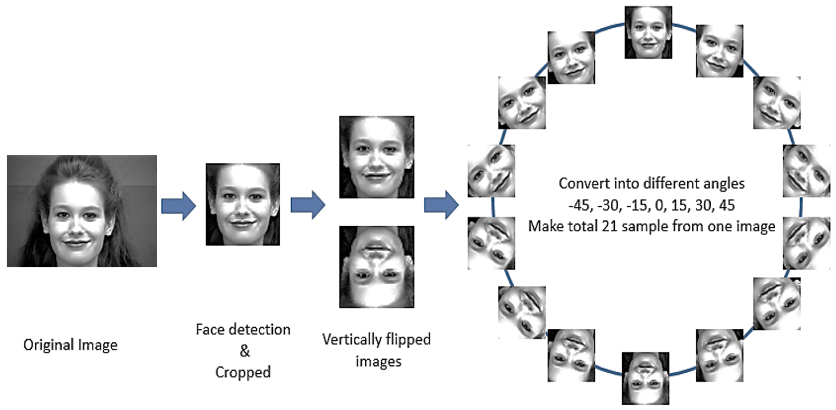
In this section, the proposed approach is presented. The mandate of the proposed approach is to consider the challenges like occlusions, illumination variations, and changes in the physical appearance of mute persons’ images and mitigate their effects. The model is designed to identify the basic expressions of human emotions such as joy, grief, surprise, fear, contempt, anger, and neutral. The proposed model is based on 6 layers of CNN, in which 5 convolutional layers are used, including the max-pooling layer and one dense layer with a dropout function. Figure 1 provides the flow of the proposed model, where preprocessing of the obtained image set is undertaken in the first step followed by face detection and cropping in the second step. In the third step, the image is flipped vertically, and 2 images and 7 angles from each image are formed producing a total of 14 images in the final step.

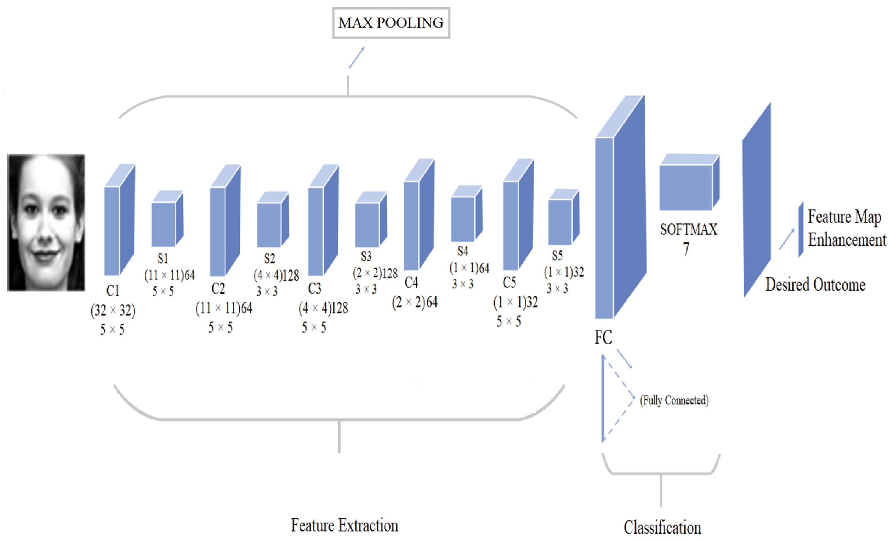
Furthermore, in the proposed framework, the first convolutional layer uses a 5 × 5 filter. It takes a 32 × 32 sized image of grayscale which means the number of channels is 1. Its output size is 32 feature maps. It breaks images into a small subsection of size 5 × 5. Then to reduce the data of the image, the max pool function is used which pools out the max value in the region as shown in Figure 2. After applying max-pooling, the size becomes 11 × 11 andbut it keeps the output size the same as the convolutional layer.

In the second layer, the output size increase from 32 × 32 to 64 × 64 with the same filter size. The input size is 11 × 11. After that, max pool volume becomes [4 × 4 × 64], while applying the third convolutional layer results in a size of [4 × 4 × 128]. The max-pooling produces a size of [2 × 2 × 128]. Now as dropping the output size of the convolutional layer begins, the output rate is reversed. In the fourth layer, after max-pooling, the CNN model makes only a 2 × 2 kernel size 64 feature map and gives [1 × 1 × 64]. In the fifth layer of convolution, the volume becomes [1 × 1 × 32] and produces 32 feature maps. The dense layer is applied with 1024 hidden neurons. A dense layer or fully connected layer changes the 2- or multi-dimensional data into flat data. All these layers use the ReLU activation function, which is actually a SoftMax function.

Machine-learning-based models have two phases training and testing/execution; in the training phase, all the data along with labels are provided to the classifier to learn from the pattern between the data and label, while in testing, the trained model is validated. The training phase runs and makes the suitable function, called $f\left(x\right)$. Initially, preprocessing is performed on the image, and features are extracted. Then CNN is applied to find the pattern and the trained model is saved. In the next phase, the trained model and weights are loaded to predict the labels for the test samples.

3.1. Dataset Description

This study uses publicly available datasets CK+ and JAFFE. These datasets have been widely used in the existing literature.

Table 2. Number of subjects and number of emotions in each database.

Detail	CK+	JAFFE
Subject	123	10
Posed emotions	8	7
Total samples	9591	213

shows the number of samples for each dataset.

CK+ has 123 subjects who posed eight emotions: anger, contempt, disgust, fear, joy, neutral, sad, and surprise. There is a sequence of images for each emotion, starting with neutral and ending with extreme expression. At this point, the images are manually picked, and then neutral images are separated from the original dataset. Similarly, the remaining images are sorted in respective folders. Now, we have 9591 total images, which also contain duplication. These duplicate images are removed, and the size of the set is reduced to 6362 images. JAFFE is based on 10 female subjects and the total number of images is 213; these images are only separated into respective folders. Detail of the total images for each emotion can be seen in

Table 3. Number of images according to the emotions in CK+ and JAFFE database original and after removing duplicates.

Emotion	Original	CK + Removing Duplicates	JAFFE	Total
Angry	1280	616	30	646
Disgust	1446	872	29	901
Fear	825	494	32	526
Happy	2187	1320	31	1351
Neutral	444	994	30	1024
Sad	1671	1080	31	1111
Surprise	1730	986	30	1016
Total	9583	6362	213	6575

. The first column represents the emotions sample. The second column has two sub-columns displaying the number of original images per set and, the number of images after removing duplicates from CK+. The third column shows JAFFE detail and the last column presents the total images of each emotion. The total number of images after removing duplication is 6575.

3.2. Preprocessing Dataset

In the preprocessing phase, the image is changed into a format that is appropriate for the CNN model. Preprocessing is dived into four main steps: detecting the face, cropping it, flipping it vertically, and making samples of different angles OpenCV [33] is used for preprocessing

In the first step, the image is converted into grayscale which converts 3-channel RGB image into 1 channel. To detect the face, Viola–Jones [34] is used with a Haar-like feature by using pre-trained cascades of frontal face files provided by OpenCV, which returns the face area. The face area is cropped and re-sized to 32 × 32 and is vertically flipped. A copy of it is then made. This step doubles the number of images which are then converted into 7 different angles (−45, −30, −15, 0, 15, 30, 45). This helps generate a large amount of image data and provides more samples to train and test. Moreover, it makes the model train at different angles as well. This process is applied in both the training set and the testing set. It makes our model more powerful and precise in detecting emotions from different angles.

CNN is well-suited for pattern classification problems. CNN is very similar to a neural network, where neurons, activation functions, weights, and learning rates are the same as a neural network. The key difference is in its structural design, as CNN takes images as input. It is specially designed to deal with 2-dimensional data [35,38]. In every CNN model, it is essential to set some hyperparameters, such as learning rates, regulation function value, filter sizes, size of the feature map, and the number of hidden neurons. All the performance of the CNN is based on these parameters and the arrangement of layers. The computation of this layer is performed by sliding a window called a filter over the original image by one pixel called stride. This process executes pixel-wise multiplication and adds up to form the result of integers, which shape individual components of the resulting matrix. The output is called a feature map, convoluted map, or activation map. The value of feature maps depends on the values of filters, as different filters generate different feature maps. We just have to initialize the parameters before the training. Following are some parameters related to different convolutional layers.

Hyperparameters are the values that should be set for training. In the current study, batch size, learning rate, weights, biases, hidden neurons, input shape, output values at each layer, etc., are hyperparameters. In this list, some are crucial, such as learning rate and hidden neurons. The batch size used is ’None’ because dynamical allocation is preferably desired. For regulation, the dropout function is used only once after the fully connected layer’s value is 0.8, and the number of hidden neurons is 1024. The learning rate of the proposed is set to 0.0001 as mentioned in

Table 4. Hyperparameters of the proposed model.

Hyperparameters	Value
Learning rate	1 × 10${}^{-9}$
Dropout	0.8
Batch size	None (dynamically allocated)
Hidden neurons	1024

.

3.3. Evaluation and Analysis

The performance of the proposed model is evaluated in terms of testing and validation. Results are evaluated regarding accuracy, which is calculated based on the values of true positive (TP), true negative (TN), false positive (FP), and false negative (FN) given in the confusion matrix.

3.4. Performance Comparison

The two recently published models are chosen to compare the performance of the proposed model. The first model, called Test Model 1 [21], consists of 3 convolutional layers. The first two layers have a 32 × 32-feature map, while the third layer has a 64 × 64-feature map. It has two fully connected layers each with 1000 hidden neurons. After every convolutional layer, max-pooling of 3 × 3 kernel is performed. The dropout rate is 0.5; the learning rate is not mentioned in the paper, so we use our learning rate (1 × 10${}^{-9}$) 0.0001 to obtain the accuracy. As per the reported results, a 96% accuracy from the model is obtained. Test Model 2 [22] is based on two convolutional layers of 32 and 64 feature maps, respectively, and one fully connected layer that has 256 hidden neurons. Max-pooling is performed after every convolutional layer with a kernel size of 2 × 2. The parameters of Test Model 1 and Test Model 2 are given in

Table 5. Hyperparameters of Test Model 1 and Test Model 2.

Hyperparameters	Test Model 1 [21]	Test Model 2 [22]
Learning rate	1 × 10${}^{-4}$	1 × 10${}^{-2}$
Dropout	0.5	N/A
Batch size	None (dynamically allocated)	None (dynamically allocated)
Hidden Neurons	1000	256

.

4. Results and Discussions

Two experiments were performed on all testing models and the proposed model; first with the combined datasets including both the CK+ and JAFFE datasets but the images and subjects are unique in training and testing datasets, while the second is based on the cross dataset in which CK+ is used for training and JAFFE for testing purposes.

4.1. Experiment 1

4.1.1. Preparation of Dataset

For experiment 1, the images are divided into training and testing data in the ratio of 0.80 to 0.2 for training and testing. As a result, the number of training samples is 5260, while the testing samples are 1315. These sets are used for preprocessing and later for classification.

To prepare the dataset, we manually label the emotions of CK+ and JAFFE databases. After labeling images, faces are detected with the help of Haar-cascades. Then the images are cropped to obtain only the face area. It reduces the area and saves on computation as well. The images are resized into 32 × 32. The dataset after prepossessing consists of 92,410 images. The training dataset is further divided into two datasets; the training set and the validation set. The training dataset is used to train the model while the validation dataset is used in training for checking the prediction accuracy during the training phase and adjusting the values of the hyperparameters accordingly. It gives an impartial evaluation of model fit on the training dataset. The test dataset is used to provide a fair evaluation of the final model fit on the training dataset.

The training dataset contains 51,562 images, the validation set contains 22,078, and the testing set contains 18,410 images. Images allocated to the training dataset are 56%, validation images make 24%, and test datasets are 20%. To make it fair while testing, data are shuffled and stored in different NumPy arrays. It takes approximately 7 to 8 min to complete the preprocessing of 92,410 images and store them in the NumPy array.

4.1.2. Training Phase

In the training phase, 32 × 32 input images are used. All models are trained and tested with the same dataset. Firstly, the training is run for 10 epochs to check the behavior of the models. The total number of iterations on the training set is 5100 and the total number of steps is 7970. First, all the models are trained to 10 epochs and the results are checked for accuracy. The proposed model takes a little time but the accuracy of the proposed model is greater as compared to the other two models. Test Model 1 is the fastest of all but not as accurate as the proposed model. Test Model 2 is neither fast nor accurate. It can be seen clearly in

Table 6. First observation after 10 epochs of training.

	Test Model 1 [21]	Test Model 2 [22]	Proposed Model
Overall accuracy	86.33%	17.2%	91.23%
Validation accuracy	83.74%	16.63%	86.57%
Overall loss	0.43776	19.06535	0.28740
Validation loss	0.46539	19.19623	0.40479

that the proposed model has higher accuracy and the least loss as compared to others. Now it is decided to train these models further.

Upon satisfaction with the performance of the proposed model, the models are trained to 100 epochs. Results are shown in

Table 7. Second observation of the first experiment after 100 epochs of training.

	Test Model 1 [21]	Test Model 2 [22]	Proposed Model
Overall accuracy	98.33%	16.29%	99.44%
Validation accuracy	92.33%	15.40%	93.20%
Overall loss	0.04361	19.27471	0.01304
Validation loss	0.44888	19.48092	0.38968

. On 100 epochs, total iterations are 51,000 and total steps are 79,700 during training. After 100 epochs, the proposed method reached an accuracy of 99.44%, and validation accuracy was 93.20%. The loss was decreased to 0.01304 and the validation loss was 0.38968 in a time of 38.104 s/epoch. Test Model 1’s accuracy was 98.33% while validation accuracy was 92.33% within 33.51 s/epochs. For Test Model 2, accuracy was 16.29%, validation accuracy was 15.40%, the loss rate was 19.2747, and validation loss was 19.4809 within 48.152 s/epochs.

4.1.3. Test Phase

To test the models, the previously created testing dataset is used for each model. Feeding the dataset into the model,

Table 8. Test result with prediction detail of Model 1 after 10 epochs.

Emotions	Dataset	Correct Prediction	Incorrect Prediction	Percentage
Anger	1792	1221	571	68.14%
Disgust	2506	1973	533	78.73%
Fear	1456	942	514	64.70%
Happy	3766	3516	250	93.36%
Neutral	2856	2099	757	73.49%
Sad	3192	2983	209	93.45%
Surprise	2842	2595	247	91.31%
Average	18,410	15,329	3081	83.26%

stats are obtained as follows.

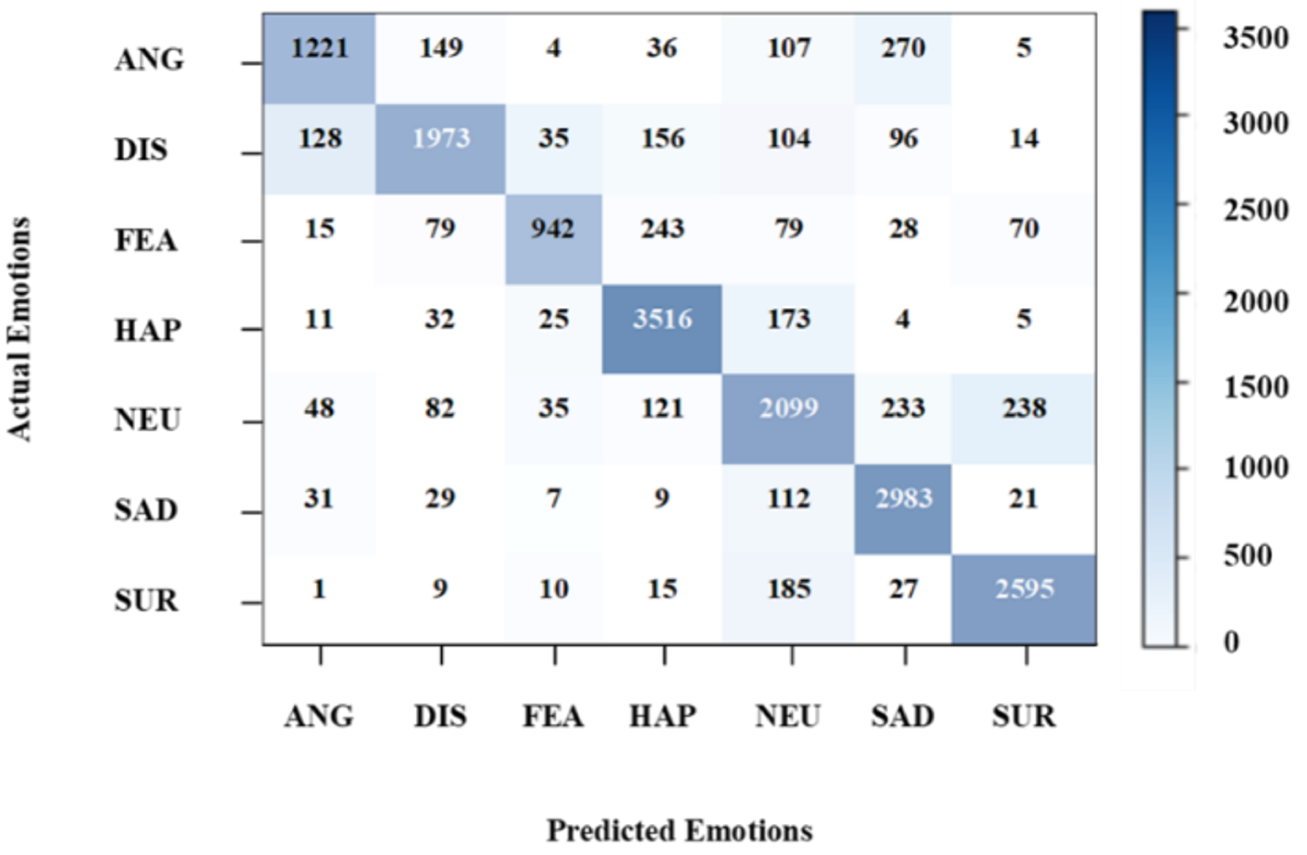
The first test is performed after 10 epochs to check the model’s accuracy on that point and confirm that the model is correct and capable of prediction. After 10 epochs, the accuracy rate of Model 1 is 83.26%. The most accurate emotion projected by Model 1 is ‘sad’ with 93.45% precision and the least accurate emotion is fear at the rate of 68.70%. However, happy, sad, and surprise emotions are above 90% accurately predicted as seen in Table 8. Then, a confusion matrix is created, as shown in Figure 3, where the accuracy of testing exceeding the comparable is clearly seen.

Test Model 2 only predicted the fear emotion with 100% accuracy and all the other emotions were mispredicted. The overall accuracy of the model is 7.91% as shown in

Table 9. Test result with prediction detail of Model 2 after 10 epochs.

Emotions	Dataset	Correct Prediction	Incorrect Prediction	Percentage
Anger	1792	0	1792	0%
Disgust	2506	0	2506	0%
Fear	1456	1456	0	100%
Happy	3766	0	3766	0%
Neutral	2856	0	2856	0%
Sad	3192	0	3192	0%
Surprise	2842	0	2842	0%
Average	18,410	1456	16,954	7.91%

. Figure 4 shows the number of correct and wrong predictions from Test Model 2 after 10 epochs. It can be seen that all emotions are misclassified except for fear.

The accuracy of the proposed model is 86.80%, as shown in

Table 10. Test result with prediction detail of the proposed model after 10 epochs.

Emotions	Dataset	Correct Prediction	Incorrect Prediction	Percentage
Anger	1792	1474	318	82.25%
Disgust	2506	1829	677	72.98%
Fear	1456	1254	202	86.13%
Happy	3766	3485	281	92.54%
Neutral	2856	2336	420	81.79%
Sad	3192	2970	222	93.05%
Surprise	2842	2632	210	92.61%
Average	18,410	15,980	2430	86.80%

. The most accurate emotion predicted by the proposed model is ‘sads at the rate of 93.05% and the least accurate emotion is ‘disgusts with a 72.98% accuracy rate. Happy, sad, and surprise emotions are predicted above 92%.

Figure 5 shows the confusion matrix of the proposed approach. Results indicate that its performance is better than both Test Model 1 and Test Model 2 on average, as it produces a higher number of correct emotions.

The comparison of all three models can be seen in

Table 11. Comparison of emotion prediction by Model 1, Model 2, and proposed model for experiment 1 after 10 epochs.

Emotions	Test Model 1 [21]	Test Model 2 [22]	Proposed Model
Anger	68.14%	0%	82.25%
Disgust	78.73%	0%	72.98%
Fear	64.70%	100%	86.13%
Happy	93.36%	0%	92.54%
Neutral	73.49%	0%	81.79%
Sad	93.45%	0%	93.05%
Surprise	91.31%	0%	92.61%
Average	83.26%	7.91%	86.80%

. After 10 epochs, the accuracy rate of Model 1 is 83.26%, Model 2 is 7.91% and the proposed model is 86.80%, which is the highest as compared to other models. The overall accuracy of the projected model is greater than other models.

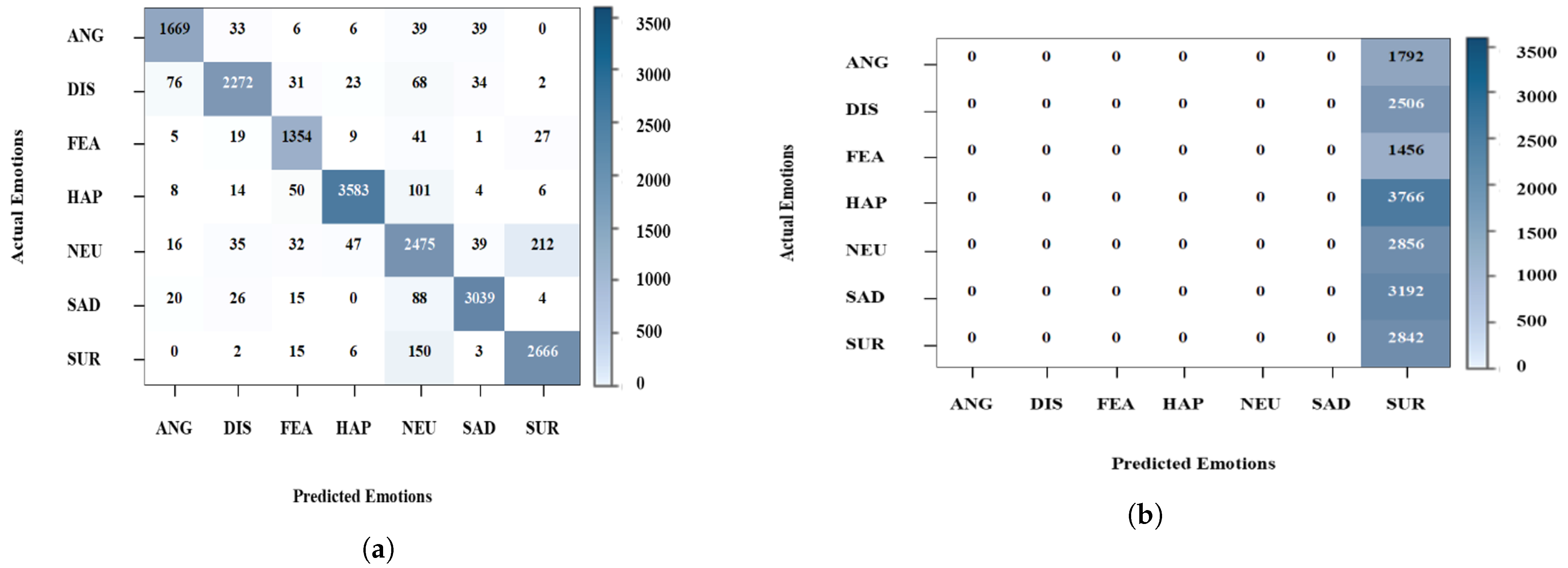
As the first test results were satisfactory, a second test was performed. The second observation was based on the test results after 100 epochs of training. The results of Test Model 1 are given in

Table 12. Test result with prediction detail of Model 1 after 100 epochs.

Emotions	Dataset	Correct Prediction	Incorrect Prediction	Percentage
Anger	1792	1667	125	93.02%
Disgust	2506	2254	252	89.94%
Fear	1456	1321	135	90.73%
Happy	3766	3583	183	95.14%
Neutral	2856	2536	320	88.79%
Sad	3192	2901	291	90.88%
Surprise	2842	2642	200	92.96%
Average	18,410	16,904	1506	91.82%

. Model 1’s accuracy is increased after 100 epochs. All the emotions are detected above 88%. The most accurately detected emotion is happy with an accuracy of 95.14%, and the least accurately detected one is neutral. The overall accuracy is 91.82%.

Test Model 2 is only capable of predicting the ’surprise’ emotion, as shown in

Table 13. Test result with prediction detail of Model 2 after 100 epochs.

Emotions	Dataset	Correct Prediction	Incorrect Prediction	Percentage
Anger	1792	0	1792	0%
Disgust	2506	0	2506	0%
Fear	1456	0	1456	0%
Happy	3766	0	3766	0%
Neutral	2856	0	2856	0%
Sad	3192	0	3192	0%
Surprise	2842	2842	0	100%
Average	18,410	2842	15,568	15.44%

. A 100% accuracy is obtained for surprise emotions while all other emotions are misclassified. The overall accuracy is 15.44%.

According to the end results of the proposed model, the most accurate emotion recognized by the proposed model is ’sad’ at the rate of 95.21%, and the least is neutral emotion with 86.66%. All the emotions have an accuracy rate higher than 86%, as shown in

Table 14. Test result with prediction detail of the proposed model after 100 epochs.

Emotions	Dataset	Correct Prediction	Incorrect Prediction	Percentage
Anger	1792	1669	123	93.14%
Disgust	2506	2272	234	90.66%
Fear	1456	1354	102	92.99%
Happy	3766	3583	183	95.14%
Neutral	2856	2475	381	86.66%
Sad	3192	3039	153	95.21%
Surprise	2842	2666	176	93.81%
Average	18,410	17,058	1352	92.66%

. Figure 6, shows the confusion matrices after 100 epochs.

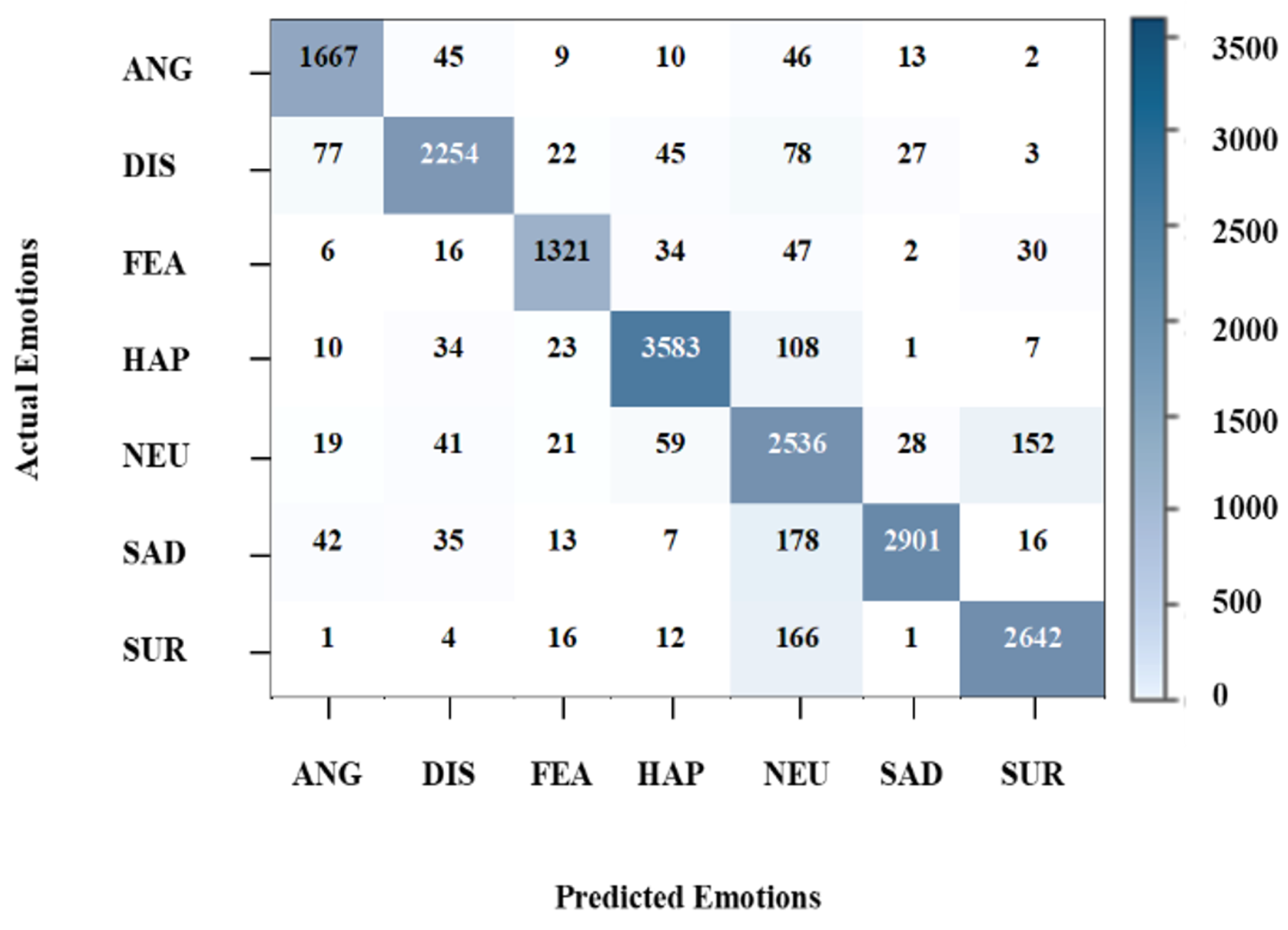
The confusion matrix for the proposed model after 100 epochs is presented in Figure 7. It indicates that the number of correct predictions is higher as compared to Test Model 1 and Test Model 2. As a result, the prediction accuracy is higher as a whole, as well as, for individual emotions.

The proposed model accuracy achieves 92.66% accuracy after 100 epochs of training. It can be seen that the proposed method and Test Model 1 predict happy emotion with the same accuracy of 95.14%. However, the proposed model predicts other emotions more correctly i.e., anger, disgust, fear, and sad as compared to Test Model 1. However, Test Model 1 more accurately predicts neutral emotion. Test Model 2 only predicts surprise emotion with 100% accuracy. A comparison of all three models regarding each emotion is given in

Table 15. Comparison of emotion prediction by Model 1, Model 2, and proposed model for experiment 1 after 100 epochs.

Emotions	Test Model 1 [21]	Test Model 2 [22]	Proposed Model
Anger	93.02%	0%	93.14%
Disgust	89.94%	0%	90.66%
Fear	90.73%	0%	92.99%
Happy	95.14%	0%	95.14%
Neutral	88.79%	0%	86.66%
Sad	90.88%	0%	95.21%
Surprise	92.96%	100%	93.81%
Average	91.82%	15.44%	92.66%

. The comparison reveals that Model 1 is faster than other models, but the proposed model is more precise and performs well, giving more accurate results.

4.2. Experiment 2

The second experiment is based on the cross-dataset evaluation. It is executed to check the performance and fair evaluation of the proposed model. It helps to observe and analyze how the models perform outside of the training dataset.

4.2.1. Preparation of Dataset

In this test, we used the CK+ dataset and JAFFE datasets separately. CK+ was split in half, one for training and the second for validation. The total images of CK+ are 6362 and after prepossessing, it generates 89,068 images. Each dataset contains 44,534 images. The JAFFE dataset is used for testing purposes, which contains 213 images, and after preprocessing, it produces 2982 images as shown in

Table 16. Division detail along with numbers of images per set for cross dataset test.

Dataset	Total	Split	Percentage	# of Images	Total Images after Preprocessing
CK+	6362	Training	50%	3181	44,534
		Validation	50%	3181	44,534
JAFFE	213	Testing	100%	213	2982

.

4.2.2. Training Phase

For training, we use the same method as in the previous experiment except for the dataset. In the testing phase, we feed the CK+ dataset, train the model, and analyze the behavior of the models. Initially, the results are checked after the completion of training up to 10 epochs. The preliminary observation was the same as before in the experiment. The proposed model took longer time than Test Model 1 but the accuracy of the model is superior to the other two models. Test Model 1 is the fastest of all but not as precise as the proposed model. Test Model 2 is neither fast nor accurate as compared to any other model.

Table 17. First observation after 10 epochs of training of experiment 2.

	Test Model 1 [21]	Test Model 2 [22]	Proposed Model
Overall accuracy	85.88%	18.93%	89.76%
Validation accuracy	84.54%	20.37%	85.64%
Overall loss	0.47114	18.6617	0.29435
Validation loss	0.44943	18.33486	0.44149
Time per epoch	35.641/s	54.904/s	41.302/s

shows the experimental results after 10 epochs. The accuracy of the proposed Model is 89.76%, and the loss is 0.29435 where Test Model 1 has 85.88% accuracy, and loss is 0.47114 and Test Model 2 gets only 18.93% accuracy and loss is 18.6617. The time of the proposed model to complete each epoch is 41.302 s where Test model 1 finishes one epoch in 35.641 s. Test Model 2 is the slowest of all with 54.904 s. It can be seen that the proposed model has higher accuracy and the least loss as compared to others.

Similar to the first experiment, the second training session is performed up to 100 epochs to evaluate models. The results of the training are shown in

Table 18. Second observation after 100 epochs of training of experiment 2.

	Test Model 1 [21]	Test Model 2 [22]	Proposed Model
Overall accuracy	98.34%	16.11%	99.40%
Validation accuracy	92.83%	17.06%	93.83%
Overall loss	0.03960	19.31624	0.01603
Validation loss	0.42293	19.09687	0.35530
Time per epoch	30.463/s	47.763/s	35.817/s

. On 100 epochs, the total number of iterations is 44,534 and the total number of steps is 69,600 during training. After the training, the proposed model achieves a 99.40% accuracy and 93.83% overall accuracy. The loss is dropped to 0.01603 and validation loss reaches 0.35530 in time of 35.817 s/epoch.

Test Model 1 obtains 98.34% accuracy and 92.83% validation accuracy. The loss rate is reduced to 0.03960 and the validation loss becomes 0.42293 within 30.463 s/epoch, whereas Test Model 2 only manages to reach the accuracy of 16.11% with a validation accuracy of 17.06%. The loss rate of this model is 19.31624 and the validation loss is 19.09687 in 47.763 s/epoch time.

4.2.3. Testing Phase

In the testing session of experiment 2, we use the JAFFE database for each model as the testing dataset. The first observation is based on training setup up to only 10 epochs. To perform this first, we feed the dataset in trained models and check the accuracy.

The results of Test Model 1, given in

Table 19. Cross dataset testing result of Test Model 1 after 10 epochs.

Emotions	Dataset	Correct Prediction	Incorrect Prediction	Percentage
Anger	420	354	66	84.29%
Disgust	406	387	19	95.32%
Fear	448	341	107	76.12%
Happy	434	413	21	95.16%
Neutral	420	213	207	50.71%
Sad	434	401	33	92.40%
Surprise	420	401	19	95.48%
Average	2982	2510	472	84.17%

, highlight the overall accuracy of this model which is 84.17%. It can identify all emotions but the most accurate one is ‘surprise’ with an accuracy rate of 95.48% and neutral emotions has the lowest accuracy of 50.71%. However, angry, happy, and sad emotions are above 84% rate.

Test Model 2 is only able to detect the ‘anger’ emotion with 100% accuracy while all other emotions are incorrectly predicted, as shown in

Table 20. Cross dataset testing result of Model 2 after 10 epochs.

Emotions	Dataset	Correct Prediction	Incorrect Prediction	Percentage
Anger	420	420	0	100%
Disgust	406	0	406	0%
Fear	448	0	448	0%
Happy	434	0	434	0%
Neutral	420	0	420	0%
Sad	434	0	434	0%
Surprise	420	0	420	0%
Average	2982	420	2562	14.08%

. The overall accuracy of the model is 14.08% only.

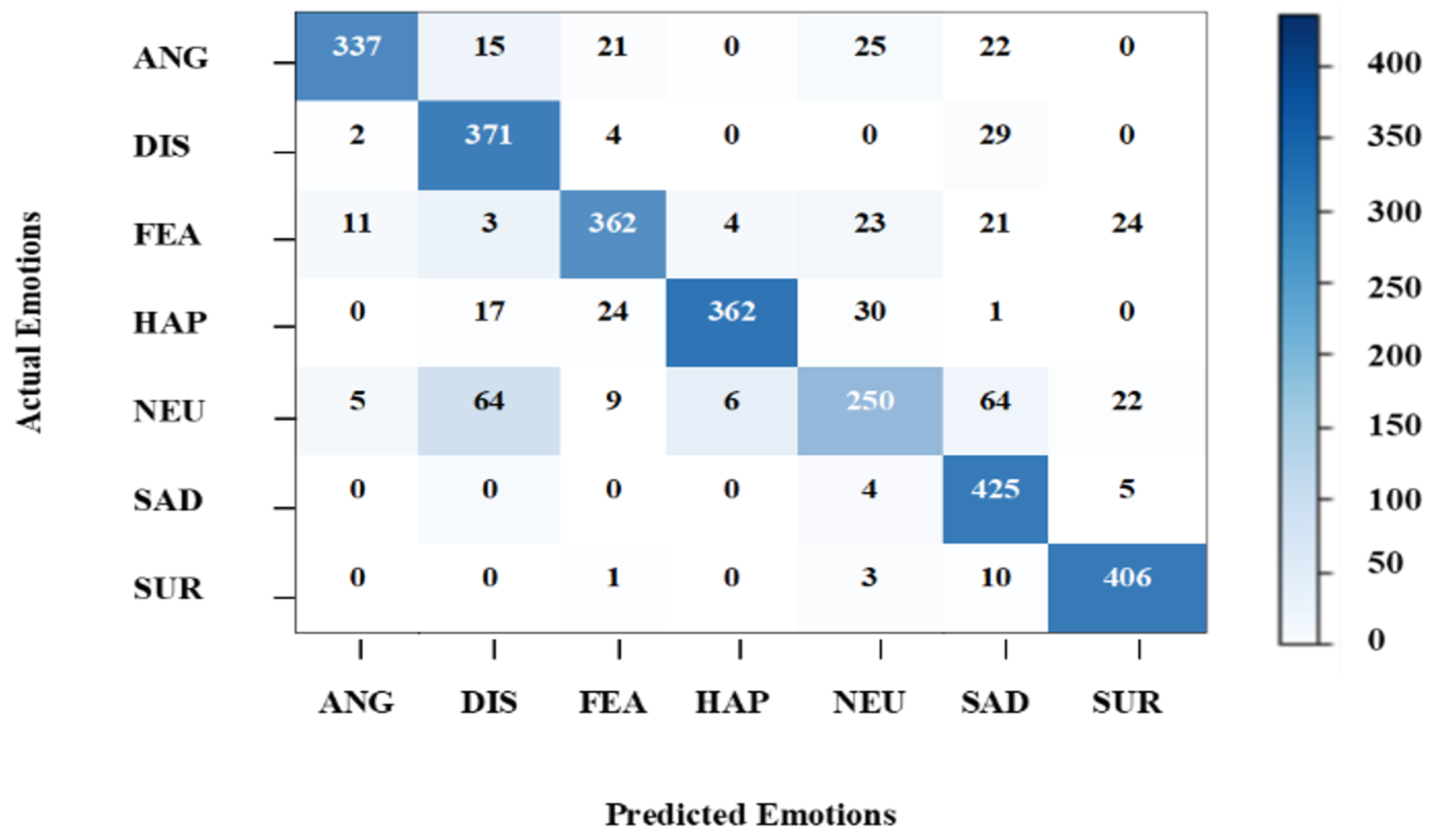
According to the results given in

Table 21. Cross dataset testing result of the proposed model after 10 epochs.

Emotions	Dataset	Correct Prediction	Incorrect Prediction	Percentage
Anger	420	337	83	80.24%
Disgust	406	371	35	91.38%
Fear	448	362	86	80.80%
Happy	434	362	72	83.41%
Neutral	420	250	170	59.52%
Sad	434	425	9	97.93%
Surprise	420	406	14	96.67%
Average	2982	2513	469	84.27%

, the overall accuracy of the proposed work is 84.27% where the highly accurate emotion is ‘sad’ with 97.93% and the lowest accuracy is for ‘neutral’ emotion, i.e., 59.52%. However, all other emotions i.e., angry, disgust, fear, happy and surprise emotions high an accuracy higher than 80%. Figure 8 shows the confusion matrix for the proposed model.

Performance comparison of all models after 10 epochs is given in

Table 22. Comparison of Test Model 1, Test Model 2, and proposed model after 10 epochs with the cross dataset.

Emotions	Test Model 1 [21]	Test Model 2 [22]	Proposed Model
Anger	84.29%	100%	80.24%
Disgust	95.32%	0%	91.38%
Fear	76.12%	0%	80.80%
Happy	95.16%	0%	83.41%
Neutral	50.71%	0%	59.52%
Sad	92.4%	0%	97.93%
Surprise	95.48%	0%	96.67%
Average	84.17%	14.08%	84.27%

which indicates that Test Model 2 performs poorly. Test Model 2 performs well; however, the performance of the proposed model is marginally better than Test Model 2 with 84.27% accuracy.

After the satisfactory results from test 1 with the cross dataset, a second test is performed which is based on one 100 epochs. After training all the models up to 100 epochs, data is tested on each model and obtain the following outcomes. Results for Test Model 1 are given in

Table 23. Cross dataset testing result of Model 1 after 100 epochs.

Emotions	Dataset	Correct Prediction	Incorrect Prediction	Percentage
Anger	420	392	28	93.33%
Disgust	406	395	11	97.29%
Fear	448	435	13	97.10%
Happy	434	412	22	94.93%
Neutral	420	320	100	76.19%
Sad	434	422	12	97.24%
Surprise	420	403	17	95.95%
Average	2982	2779	204	93.19%

. According to the end result of the test, the total accuracy of Test Model 1 is 93.16%. The most precise sentiment detected is ’disgust’ with 97.29% accuracy and the least detected emotion is neutral with 76.19% accuracy.

Results for Test Model 2 are given in

Table 24. Cross dataset testing result of Model 2 after 100 epochs.

Emotions	Dataset	Correct Prediction	Incorrect Prediction	Percentage
Anger	420	0	420	0%
Disgust	406	0	406	0%
Fear	448	0	448	0%
Happy	434	0	434	0%
Neutral	420	0	420	0%
Sad	434	434	0	100%
Surprise	420	0	420	0%
Average	2982	434	2548	14.55%

. Results indicate that Test Model 2 predicts only the ’sad’ emotion with a 100% accuracy while the accuracy for all other emotions is 0. The average accuracy of Test Model 2 for all emotions is 14.55%.

Table 25. Cross dataset testing result of the proposed model after 100 epochs.

Emotions	Dataset	Correct Prediction	Incorrect Prediction	Percentage
Anger	420	405	15	96.43%
Disgust	406	391	15	96.31%
Fear	448	434	14	96.88%
Happy	434	412	22	94.93%
Neutral	420	354	66	84.29%
Sad	434	434	0	100%
Surprise	420	401	19	95.48%
Average	2982	2831	151	94.94%

shows the results of the proposed model after 100 epochs. The proposed model is capable of detecting ’sad’ emotion with 100% accuracy, whereas other sentiments are identified with 94% or higher accuracy except for the ’neutral’ emotion with an accuracy of 84.29%.

According to the observation of test 2 based on the cross dataset with 100 epochs, Test Model 1 is adequate to distinguish emotions like disgust, fear, and surprise at a higher rate whereas happy emotion is detected at the same rate by Test Model 1 and the proposed model. The proposed model, on the other hand, recognizes anger, neutral and surprise faces more correctly, as shown in

Table 26. Comparison of Test Model 1, Test Model 2, and proposed model after 100 epochs with cross dataset.

Emotions	Test Model 1 [21]	Test Model 2 [22]	Proposed Model
Anger	93.33%	0%	96.43%
Disgust	97.29%	0%	96.31%
Fear	97.10%	0%	96.88%
Happy	94.93%	0%	94.93%
Neutral	76.19%	0%	84.29%
Sad	97.24%	100%	100%
Surprise	95.95%	0%	95.48%
Average	93.19%	14.55%	94.94%

.

The overall accuracy rate of the proposed model is 94.94%. Test Model 1 predicted emotions above 76% and up to 97.29%, whereas the proposed model predicted all emotions above 84% and up to 100% accuracy. The overall accuracy of Model 1 is 93.19%, which is less than that of the proposed model.

4.3. Discussions

To compare the results, the precision of all models is considered. Precision is calculated with the following equation:

$$Precision=\frac{TP}{TP+FP}$$

(1)

Table 27. Precision comparison between all three models with respect to observation 1 of Experiment 1 with epochs 10.

Emotions	Test Model 1 [21]	Test Model 2 [22]	Proposed Model
Anger	0.8392	0.0000	0.7916
Disgust	0.8385	0.0000	0.9375
Fear	0.8904	0.0791	0.7642
Happy	0.8584	0.0000	0.9378
Neutral	0.7342	0.0000	0.7781
Sad	0.8193	0.0000	0.9016
Surprise	0.8803	0.0000	0.8940
Average	0.8372	0.0113	0.8578

tells us about the comparison between models and experiments of observation 1 for experiment 1. According to the given results, the average precision of the proposed model is higher (0.8578) than other models (0.8372 for Test Model 1 and 0.0113 for Test Model 2).

For experiment 2, observation 1, the proposed model has an average precision of 0.8499, whereas Test Model 1 has 0.8488 precision, as shown in

Table 28. Precision comparison between all three models with respect to observation 1 of Experiment 2 with 10 epochs.

Emotions	Test Model 1 [21]	Test Model 2 [22]	Proposed Model
Anger	0.8806	0.1408	0.9493
Disgust	0.6661	0.0000	0.7894
Fear	0.9394	0.0000	0.8599
Happy	0.8463	0.0000	0.9731
Neutral	0.7448	0.0000	0.7463
Sad	0.8911	0.0000	0.7430
Surprise	0.9733	0.0000	0.8884
Average	0.8488	0.0201	0.8499

. Test Model 2 shows the lowest precision in both experiments. In experiment 1, the proposed model is able to predict five emotions, disgust, happy, neutral, sad, and surprise, more precisely than other models. A similar trend is observed in the case of experiment 2.

Observation 2 of both experiments is given in

Table 29. Precision comparison between all three models with respect to observation 2 of Experiment 1 with 100 epochs.

Emotions	Test Model 1 [21]	Test Model 2 [22]	Proposed Model
Anger	0.9149	0.0000	0.9303
Disgust	0.9280	0.0000	0.9463
Fear	0.9270	0.0000	0.9009
Happy	0.9555	0.0000	0.9752
Neutral	0.8028	0.0000	0.8356
Sad	0.9758	0.0000	0.9620
Surprise	0.9264	0.1544	0.9140
Average	0.9186	0.0221	0.9235

and

Table 30. Precision comparison between all three models with respect to observation 2 of Experiment 2 with 100 epochs.

Emotions	Test Model 1 [21]	Test Model 2 [22]	Proposed Model
Anger	0.9874	0.0000	0.9712
Disgust	0.8624	0.0000	0.9354
Fear	0.9603	0.0000	0.9819
Happy	0.9258	0.0000	0.9649
Neutral	0.8696	0.0000	0.8939
Sad	0.9357	0.1455	0.9079
Surprise	0.9829	0.0000	0.9926
Average	0.9320	0.0208	0.9614

, respectively. It can be observed that the precision of the proposed model is higher than other models. The average precision of the proposed model in experiment 1 is 0.9235, and that of Test Model 1 is 0.9186. In experiment 2, the proposed model has a precision of 0.9614 and Test Model 1 has a precision of 0.9320. Test Model 2 has a precision of 0.0221 and 0.0208, respectively.

In observation 2 of experiment 1, the proposed model is more precise for emotions of anger, disgust, happy and neutral whereas, in experiment 2, disgust fear neutral, sad, and surprise is more accurate than the others. The proposed model takes a slightly longer time than Test Model 1 but it is faster than Test Model 2 and more accurate than both models. It achieved up to 92.66% accuracy in experiment 1 and 94.94% in experiment 2 based on the cross dataset.

5. Conclusions and Future Work

A new architecture design for a convolutional neural network is presented in this study for facial expression recognition. By changing the arrangement of the layer and applying a 1 × 10${}^{-4}$ learning rate, substantial improvement in the precision of the model has been accomplished. Extensive experiments are performed using CK+ and JAFFE datasets. Two strategies are used for experiments, wherein the first involves using CK+ and JAFFE datasets as one dataset, while for the second, CK+ is used for training and validation, and JAFEE is used for testing. Performance is evaluated at different epoch levels and other hyperparameters. Experimental results suggest that the proposed model shows superior performance compared to both models used for performance comparison. The proposed model achieves average accuracy scores of 92.66% and 94.94% for experiments 1 and 2, respectively. To deal with the occlusion and posture change, the images are generated at different angles, and results indicate that the proposed model is able to detect emotions at 45${}^{\circ }$. Despite the better results using the proposed model, it is limited to not using dark-colored faces and dark images for emotion detection.

In the future, we intend to make an application using the proposed model that can detect emotions for patients with autism spectrum disorder, who face difficulty in expressing emotions and social interaction. It will help them to communicate with others and can be of great help for diagnostic and therapeutic services. This application scans the person and can translate their intuitions and emotions for other people. It can be extensively used by medical practitioners, therapists, and psychologists who primarily work with people with mental illnesses, developmental disabilities, and neurological disorders, hence providing a great service to society and humanity.

References

1. Ekman, P.; Friesen, W.V.; Ellsworth, P. Emotion in the Human Face: Guidelines for Research and An Integration of Findings; Elsevier: Amsterdam, The Netherlands, 2013; Volume 11. [Google Scholar]
2. Dalgleish, T.; Power, M. Handbook of Cognition and Emotion; John Wiley & Sons: Hoboken, NJ, USA, 2000. [Google Scholar]
3. Ekman, P.; Friesen, W.V. Facial action coding system. Environ. Psychol. Nonverbal Behav. 1978. [Google Scholar] [CrossRef]
4. Gavrilescu, M.; Vizireanu, N. Predicting depression, anxiety, and stress levels from videos using the facial action coding system. Sensors 2019, 19, 3693. [Google Scholar] [CrossRef] [PubMed] [Green Version]
5. Salmam, F.Z.; Madani, A.; Kissi, M. Facial expression recognition using decision trees. In Proceedings of the 2016 13th International Conference on Computer Graphics, Imaging and Visualization (CGiV), Beni Mellal, Morocco, 29 March–1 April 2016; pp. 125–130. [Google Scholar]
6. Yang, M.H.; Kriegman, D.J.; Ahuja, N. Detecting faces in images: A survey. IEEE Trans. Pattern Anal. Mach. Intell. 2002, 24, 34–58. [Google Scholar] [CrossRef] [Green Version]
7. Berbar, M.A.; Kelash, H.M.; Kandeel, A.A. Faces and facial features detection in color images. In Proceedings of the Geometric Modeling and Imaging–New Trends (GMAI’06), London, UK, 5–7 July 2006; pp. 209–214. [Google Scholar]
8. Mostafa, A.; Khalil, M.I.; Abbas, H. Emotion recognition by facial features using recurrent neural networks. In Proceedings of the 2018 13th International Conference on Computer Engineering and Systems (ICCES), Cairo, Egypt, 18–19 December 2018; pp. 417–422. [Google Scholar]
9. Rusia, M.K.; Singh, D.K.; Ansari, M.A. Human face identification using lbp and haar-like features for real time attendance monitoring. In Proceedings of the 2019 Fifth International Conference on Image Information Processing (ICIIP), Shimla, India, 15–17 November 2019; pp. 612–616. [Google Scholar]
10. Paul, T.; Shammi, U.A.; Ahmed, M.U.; Rahman, R.; Kobashi, S.; Ahad, M.A.R. A study on face detection using viola-jones algorithm in various backgrounds, angles and distances. Int. J. Biomed. Soft Comput. Hum. Sci. Off. J. Biomed. Fuzzy Syst. Assoc. 2018, 23, 27–36. [Google Scholar]
11. Al-Tuwaijari, J.M.; Shaker, S.A. Face Detection System Based Viola-Jones Algorithm. In Proceedings of the 2020 6th International Engineering Conference “Sustainable Technology and Development” (IEC), Erbil, Iraq, 26–27 February 2020; pp. 211–215. [Google Scholar]
12. Tivatansakul, S.; Ohkura, M. The design, implementation and evaluation of a relaxation service with facial emotion detection. In Proceedings of the 2014 IEEE Symposium on Computational Intelligence in Healthcare and e-Health (CICARE), Orlando, FL, USA, 9–12 December 2014; pp. 40–47. [Google Scholar]
13. Happy, S.; Routray, A. Automatic facial expression recognition using features of salient facial patches. IEEE Trans. Affect. Comput. 2014, 6, 1–12. [Google Scholar] [CrossRef] [Green Version]
14. Ashwin, T.; Jose, J.; Raghu, G.; Reddy, G.R.M. An e-learning system with multifacial emotion recognition using supervised machine learning. In Proceedings of the 2015 IEEE Seventh International Conference On Technology for Education (T4E), Warangal, India, 10–13 December 2015; pp. 23–26. [Google Scholar]
15. Roshanzamir, M.; Alizadehsani, R.; Roshanzamir, M.; Shoeibi, A.; Gorriz, J.M.; Khosrave, A.; Nahavandi, S. What happens in Face during a facial expression? Using data mining techniques to analyze facial expression motion vectors. arXiv 2021, arXiv:2109.05457. [Google Scholar]
16. Yao, L.; Wan, Y.; Ni, H.; Xu, B. Action Unit Classification for Facial Expression Recognition Using Active Learning and SVM. Multimed. Tools Appl. 2021, 80, 24287–24301. [Google Scholar] [CrossRef]
17. Mehendale, N. Facial Emotion Recognition Using Convolutional Neural Networks (FERC); Springer: Berlin/Heidelberg, Germany, 2021; Volume 2, pp. 1–8. [Google Scholar]
18. Akhand, M.; Roy, S.; Siddique, N.; Kamal, M.A.S.; Shimamura, T. Facial emotion recognition using transfer learning in the deep CNN. Electronics 2021, 10, 1036. [Google Scholar] [CrossRef]
19. Ghimire, D.; Lee, J. Geometric feature-based facial expression recognition in image sequences using multi-class adaboost and support vector machines. Sensors 2013, 13, 7714–7734. [Google Scholar] [CrossRef] [PubMed] [Green Version]
20. Bost, R.; Popa, R.A.; Tu, S.; Goldwasser, S. Machine learning classification over encrypted data. Cryptol. Eprint Arch. 2014. Available online: https://www.ndss-symposium.org/ndss2015/ndss-2015-programme/machine-learning-classification-over-encrypted-data/ (accessed on 8 November 2022).
21. Xiao, H.; Li, W.; Zeng, G.; Wu, Y.; Xue, J.; Zhang, J.; Li, C.; Guo, G. On-Road Driver Emotion Recognition Using Facial Expression. Appl. Sci. 2022, 12, 807. [Google Scholar] [CrossRef]
22. Soleymani, M.; Asghari-Esfeden, S.; Fu, Y.; Pantic, M. Analysis of EEG signals and facial expressions for continuous emotion detection. IEEE Trans. Affect. Comput. 2015, 7, 17–28. [Google Scholar] [CrossRef]
23. Jaiswal, S.; Nandi, G.C. Robust real-time emotion detection system using CNN architecture. Neural Comput. Appl. 2020, 32, 11253–11262. [Google Scholar] [CrossRef]
24. Radlak, K.; Smolka, B. High dimensional local binary patterns for facial expression recognition in the wild. In Proceedings of the 2016 18th Mediterranean Electrotechnical Conference (MELECON), Lemesos, Cyprus, 18–20 April 2016; pp. 1–5. [Google Scholar]
25. Li, S.; Deng, W. Real world expression recognition: A highly imbalanced detection problem. In Proceedings of the 2016 International Conference on Biometrics (ICB), Halmstad, Sweden, 13–16 June 2016; pp. 1–6. [Google Scholar]
26. Kiran, T.; Kushal, T. Facial expression classification using Support Vector Machine based on bidirectional Local Binary Pattern Histogram feature descriptor. In Proceedings of the 2016 17th IEEE/ACIS International Conference on Software Engineering, Artificial Intelligence, Networking and Parallel/Distributed Computing (SNPD), Shanghai, China, 30 May–1 June 2016; pp. 115–120. [Google Scholar]
27. Muttu, Y.; Virani, H. Effective face detection, feature extraction & neural network based approaches for facial expression recognition. In Proceedings of the 2015 International Conference on Information Processing (ICIP), Pune, India, 16–19 December 2015; pp. 102–107. [Google Scholar]
28. Pauly, L.; Sankar, D. A novel online product recommendation system based on face recognition and emotion detection. In Proceedings of the 2015 International Conference on Control, Instrumentation, Communication and Computational Technologies (ICCICCT), Kumaracoil, India, 18–19 December 2015; pp. 329–334. [Google Scholar]
29. Anil, J.; Suresh, L.P. Literature survey on face and face expression recognition. In Proceedings of the 2016 International Conference on Circuit, Power and Computing Technologies (ICCPCT), Nagercoil, India, 18–19 March 2016; pp. 1–6. [Google Scholar]
30. Corneanu, C.A.; Simón, M.O.; Cohn, J.F.; Guerrero, S.E. Survey on rgb, 3d, thermal, and multimodal approaches for facial expression recognition: History, trends, and affect-related applications. IEEE Trans. Pattern Anal. Mach. Intell. 2016, 38, 1548–1568. [Google Scholar] [CrossRef] [PubMed] [Green Version]
31. Boser, B.E.; Guyon, I.M.; Vapnik, V.N. A training algorithm for optimal margin classifiers. In Proceedings of the Fifth Annual Workshop on Computational Learning Theory, Pittsburgh, PA, USA, 27–29 July 1992; pp. 144–152. [Google Scholar]
32. Haykin, S. Neural Networks and Learning Machines, 3/E; Pearson Education India: Noida, India, 2009. [Google Scholar]
33. Rudovic, O.; Pantic, M.; Patras, I. Coupled Gaussian processes for pose-invariant facial expression recognition. IEEE Trans. Pattern Anal. Mach. Intell. 2012, 35, 1357–1369. [Google Scholar] [CrossRef] [PubMed] [Green Version]
34. Jeni, L.A.; Girard, J.M.; Cohn, J.F.; De La Torre, F. Continuous au intensity estimation using localized, sparse facial feature space. In Proceedings of the 2013 10th IEEE International Conference and Workshops on Automatic Face and Gesture Recognition (FG), Shanghai, China, 22–26 April 2013; pp. 1–7. [Google Scholar]
35. Fnaiech, A.; Sayadi, M.; Gorce, P. Feature points tracking and emotion classification. In Proceedings of the 2016 2nd International Conference on Advanced Technologies for Signal and Image Processing (ATSIP), Monastir, Tunisia, 21–23 March 2016; pp. 172–176. [Google Scholar]
36. Ijjina, E.P.; Mohan, C.K. Facial expression recognition using kinect depth sensor and convolutional neural networks. In Proceedings of the 2014 13th International Conference on Machine Learning and Applications, Detroit, MI, USA, 3–6 December 2014; pp. 392–396. [Google Scholar]
37. Zhang, K.; Huang, Y.; Du, Y.; Wang, L. Facial expression recognition based on deep evolutional spatial-temporal networks. IEEE Trans. Image Process. 2017, 26, 4193–4203. [Google Scholar] [CrossRef] [PubMed]
38. Chu, C.C.; Chen, D.Y.; Hsieh, J.W. Low-cost facial expression on mobile platform. In Proceedings of the 2015 International Conference on Machine Learning and Cybernetics (ICMLC), Guangzhou, China, 12–15 July 2015; Volume 2, pp. 586–590. [Google Scholar]
Figure 1. Workflow of the proposed methodology.
Applsci 12 11797 g001
Figure 2. Architecture of the proposed model.
Applsci 12 11797 g002
Figure 3. Confusion matrix of Test Model 1 after 10 epochs.
Applsci 12 11797 g003
Figure 4. Confusion matrix of Test Model 2 after 10 epochs.
Applsci 12 11797 g004
Figure 5. Confusion matrix of the proposed model after 10 epochs.
Applsci 12 11797 g005
Figure 6. Confusion matrices after 100 epochs, (a) Test Model 1, and (b) Test Model 2.
Applsci 12 11797 g006
Figure 7. Confusion matrix of the proposed model after 100 epochs.
Applsci 12 11797 g007
Figure 8. Confusion matrix of the proposed model performed with cross dataset after 10 epochs.
Applsci 12 11797 g008