Abstract
The mismatch of geometric parameters in a nanotomography system bears a significant impact on the reconstructed images. Moreover, projection image noise is increased due to limitations of the X-ray power source. The accuracy of the existing self-calibration method, which uses only the grayscale information of the projected image, is easily affected by noise and leads to reduced accuracy. This paper proposes a geometric parameter self-calibration method based on feature matching of mirror projection images. Firstly, the fast extraction and matching feature points in the mirror projection image are performed by speeded-up robust features (SURF). The feature triangle is then designed according to the stable position of the system’s rotation axis to further filter the feature points. In turn, the influence of the mismatched points on the calculation accuracy is reduced. Finally, the straight line where the rotation axis is located is fitted by the midpoint coordinates of the filtered feature points, thereby realizing geometric parameter calibration of the system. Simulation and actual data from the experimental results show that the proposed method effectively realizes the calibration of geometric parameters, and the blurring and ghosting caused by geometric artifacts are corrected. Compared with existing methods, the image clarity can be improved by up to 14.4%.
1. Introduction
Nanotomography is a technique that uses the attenuation-based information from X-rays after penetrating an object to achieve high-resolution three-dimensional imaging of the object’s internal structure [1]. It has the advantages of nondestructive imaging, high-resolution accuracy, and fast imaging speed. It is widely used in fields such as nondestructive testing [2], material analysis [3], and 3D printing [4]. However, the mismatch between the actual spatial structure parameters of the system and the ideal model parameters leads to the generation of geometric artifacts. The blurring and ghosting in 3D reconstruction images seriously affect image information acquisition. The calibration of geometric parameters presents the foundation for obtaining high-quality 3D-reconstructed images. Therefore, the calibration of geometric parameters is essential.
Researchers have recently proposed and developed many methods for calibrating the geometric parameters of CT systems. They can be divided into the phantom-based geometric parameter calibration method, the geometric parameter self-calibration method based on reconstructed image features, and the geometric parameter self-calibration method based on projected image features. The basic principle underlying the phantom-based method is the use of standard templates with known geometric shapes. The system’s geometric parameters are then solved using the phantom projection trajectory calculation parameters [5,6,7,8]. This method has the advantages of high correction accuracy and fast solution speed. However, this method requires the fabrication and placement of a high-precision calibration phantom, consequently making its application difficult in nanotomography which uses a single-imaging field of only a few millimeters.
The geometric parameter self-calibration method based on reconstructing image features uses the reconstructed image feature information of the detected object to construct a criterion to calibrate geometric parameters. In 2007, Mayo et al. [9] proposed a cross-correlation-based software correction method to correct the blurred reconstructed image caused by image misalignment. In 2008, Kyriakou et al. [10] proposed to reconstruct the image entropy information to minimize the correction of geometric artifacts. In 2010, Kingston et al. [11] proposed reconstruction of the image sharpness minimization to achieve geometric parameter calibration. When the image texture is complex, the correction effect of entropy and sharpness methods conspicuously decreases. In 2013, Tan et al. [12] applied the idea of interval division to divide the solution parameters into multiple cells, and iteratively narrowed the interval by comparing the reconstructed image quality corresponding to the endpoint values of the interval, thus realizing the solution of the geometric parameters of a CT system. In 2017, Yang et al. [13] proposed a classification network based on deep learning to classify reconstructed image slices into geometric artifacts and non-geometric artifacts to achieve artifact correction. In 2021, Xiao et al. [14] proposed a deep neural network containing six-layer convolution and six-layer deconvolution to achieve the correction of geometric artifacts in a data-driven manner. The deep-learning-based method provides a new idea for geometric artifact correction. However, the technique requires extensive data for network training. The method based on the reconstruction of image features requires multiple iterative reconstruction, and the correction efficiency is low.
The geometric calibration method based on the projected image feature directly uses object projection information to realize the calibration of geometric parameters. In 2008, Panetta et al. [15] extended the redundancy of the sinusoidal curve projected by fan-beam CT in the central plane to cone-beam CT projection data, using the redundancy of projected data to construct cost functions to realize geometric parameter calibration. In 2009, Patel et al. [16] used the symmetry relationship between mirror projection images with a 180-degree difference to construct a cost function for correcting the deflection angle and lateral offset of the axis of rotation. In 2013, Meng et al. [17] corrected the geometric parameters of the cone beam CT system using projection and symmetry. This method proves that the sum of the projection images centered on the axis of rotation is symmetrical, and the geometric parameters of the five systems are corrected by minimizing the symmetry error of the projection and the rotation. In 2018, Xiao et al. [18] proposed a self-calibration method for geometric parameters based on the immovability of the rotating axis. This method uses the center-row and center-column of the symmetrical projection image to construct a similarity function to achieve geometric parameter correction. In 2019, Lin et al. [19] proposed a method based on sinogram symmetry to determine parameters by calculating the minimum value of the variance between the left-half of the virtual detector and the right-half of the projected data sum. These methods realize parameter calibration based on projected image and have low computational complexity. However, the direct use of the projection image grayscale value for geometric parameter calculation is susceptible to noise and cone angle of the cone beam, which reduces calculation accuracy.
In this study, a method based on projected feature matching is proposed to achieve geometric parameter self-calibration. Firstly, the feature-point-based image alignment algorithm in feature matching is advantageously utilized to realize the mirror projection image for feature-point extraction and matching. Secondly, the feature triangles are designed based on the immovable position of the rotation axis to realize fine screening of the feature-point pairs and reduce the impact of mismatched points on the calculation accuracy. Third, the random sample consistency algorithm (RANSAC) [20] is used to fit the position of the rotation axis. Finally, calibration of the lateral offset of the rotation axis and the deflection angle of the rotation axis is achieved. Simulations and actual data show that the method achieves good results in calibrating geometric parameters and can effectively eliminate the blurring and ghosting caused by geometric artifacts.
The rest of this paper is organized as follows. The geometric model of the nanotomography and the proposed method are introduced in detail in Section 2. In Section 3, the feasibility and accuracy of the method are verified by simulation and nanotomography experimentation and compared with other methods. Finally, concluding remarks are provided in Section 4.
2. Materials and Methods
2.1. System Structure and Geometric Srtifacts
The nanotomography system consists of a cone beam X-ray source, a mechanical platform, a detector, and a computer control system. We built the coordinate system shown in Figure 1 to describe the geometry of the nanotomography system more clearly. Ideally, the geometry satisfies both of the following relationships: (1) The center ray is perpendicular to the plane where the detector is located and intersects with the detector center; (2) The plane composed of the rotation axes and is parallel to the plane where the detector is located, and the projection of the rotation axis on the detector is the center column of the detector, that is, the straight line where is located. The geometric parameters of a nanotomography system can be expressed using the seven parameters shown in Table 1.
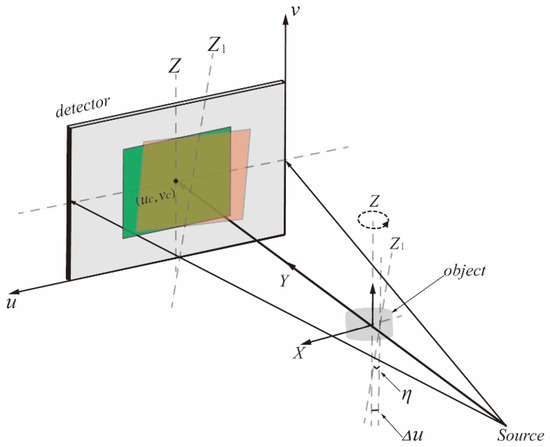
Figure 1.
Geometric model of a laboratory nanotomography system.

Table 1.
Geometric parameters of nanotomography system.
Any deviation between the geometric parameters of the actual nanotomography system and the ideal geometric relation model will produce geometric artifacts. The geometric artifacts in the reconstructed image mainly show blurring and ghosting. The details of the reconstructed image are lost, making it difficult to obtain useful information from the image. In practice, not all misaligned parameters will have the same effect on the quality of the reconstructed image. The defined in Table 1 and the lateral offset of the rotation axis shown in Figure 1 have a more serious impact on the system [1,3,21,22]. This paper mainly calibrates these two parameters with significant influence.
2.2. Geometric Parameter Calibration Process
The nanotomography geometric parameter self-calibration algorithm based on projection feature matching mainly includes projection image preprocessing, pairwise projection image registration based on feature points, and solving geometric parameters. The flow of geometric parameters is shown in Figure 2. The preprocessing of projected images mainly uses the normalization of projected image gray value, non-local average denoising and histogram equalization. Feature-matching screening is mainly achieved by extracting feature points from SURF and designing feature triangles from projection images. The filtered high-quality matching feature points are then used to achieve the proposed parameter fitting, and the parameters are used to achieve projection correction. Finally, 3D reconstruction of the projection image using the Feldkamp–Davis–Kress (FDK) reconstruction algorithm is used to obtain the voxel data.
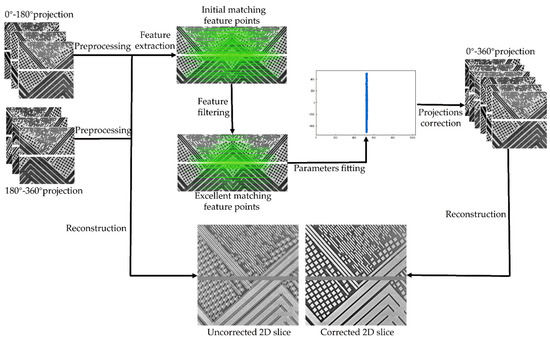
Figure 2.
The parameter calibration flow of the proposed method.
2.2.1. Projection Image Preprocessing
Firstly, the mirror projection images are linearly transformed to normalize the gray value of the projected image. The normalized projected image is then denoised by a non-local average denoising algorithm to reduce the influence of noise on the algorithm. Finally, histogram equalization is applied to enhance the contrast. The preprocessing of projection images improves image quality and contrast, which lays the foundation for more accurate projection feature extraction and matching.
2.2.2. Projection Image Processing
The SURF algorithm is a fast and robust image recognition and description algorithm that uses Hessian matrices to detect feature points and accelerate operations using integral graphs [23]. The SURF algorithm extracts feature points in the projected image. The feature points are then matched between the feature-point pairs by the Fast Library for Approximate Nearest Neighbors (FLANN) algorithm [24]. Due to noise and brightness, some feature-point pairs of projected images are mismatched. A feature-point screening algorithm for projected images under a circular scanning trajectory is designed to establish a more reliable matching point pair.
This paper employs the characteristics of triangles composed of feature points in two projection images with a difference of 180° to achieve feature-point screening. The schematic diagram is shown in Figure 3.
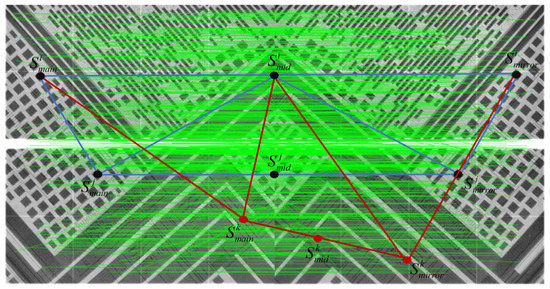
Figure 3.
Schematic diagram of feature-point screening.
Suppose that the set of feature points composed of two images with a difference of 180° is, respectively, and . Since the projected images of a CT imaging system with 180° difference under circular scanning trajectory have mirroring characteristics, when we place two images in the same coordinate system, ideally the midpoints of correctly matched feature-point pairs on the two projected images are located on the rotation axis. Thus, we can select two pairs of feature points and from the two feature point sets. These two pairs of feature points and the midpoint of one of the pairs of then form a feature triangle. are the feature point coordinates. The two triangles are equal when the feature points match correctly. Based on these points, it is possible to calculate the distance between any two points as follows:
In the same way, , , , , can be calculated. From the full equality of the feature-point triangle, it can be concluded:
However, in practical applications, it is difficult to strictly meet this equation due to the influence of noise between projections with a difference of 180°. Therefore, using the difference and setting thresholds to filter the feature pairs, the formula is converted as follows:
Set the threshold and build the criterion function such that:
And according to the criterion function construct voting function , set the voting ratio so that after filtering:
where indicates the midpoint of all feature-point pairs after filtering. is the number of the feature points.
Finally, the midpoint coordinates are parameters fitted by feature points that are less than the threshold and satisfy the voting ratio.
2.2.3. Parameter Fitting and Projection Correction
Ideally, the midpoints of all correctly matched feature-point pairs should be located on the rotation axis. So, the line where the rotation axis can be fitted by the feature-point set composed of the midpoints of the screened feature-point pairs. In this paper, the RANSAC algorithm is used to fit the rotation axis. The deflection angle of the rotation axis and the lateral deviation of the rotation axis are then solved. Finally, an affine transformation is used to correct the rotation axis deflection angle and lateral deviation of the projection data at all angles. When both the lateral deflection of the rotation axis and the angle of deflection of the rotation axis exist , the correspondence between the point after the deflection and the point before the deflection is:
Finally, the projection data after affine transformation is reconstructed to obtain 3D volume data without geometric artifacts.
3. Experiment
3.1. Simulation Experiments
This paper uses Head data as simulation data to validate and evaluate the proposed geometric parameter calibration method. The 360-projection data were generated with a step size of a 1-degree interval, and projection data with definite geometric parameter deviation and projection data without geometric parameter deviation were generated by changing parameters. The reconstructed image of the calculated geometric parameters is compared with the reconstructed image of the actual set truth value to verify the validity and accuracy of the proposed method.
As can be seen from Table 2, the calibration results of the proposed method for geometric parameters are closer to the true value parameters. Figure 4 shows the 2D slices obtained by 3D reconstruction of the true parameters, uncorrected parameters, parameters calculated by Xiao et al.’s and RANSAC method, and parameters calibrated by this method. It can be seen from the figure that there are no obvious geometric artifacts in the calibration results of the three methods. Compared with the uncorrected image, the quality of the reconstructed image is significantly improved. To better demonstrate the correction effect, Figure 5 shows the pixel values of the red line position in Figure 4. As shown in Figure 5, due to the slight deviation between RANSAC, the proposed method, and the true value parameters, the reconstruction results basically coincide with the true value results. In addition, the method proposed in this paper is closer to the pixel values of corresponding points in the results of truth-value parameter reconstruction.
Table 2.
The calibration parameters in the Head data compared with the true value, Xiao [18], RANSAC and ours.
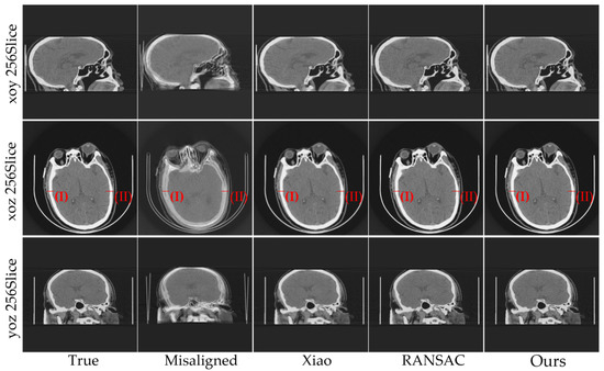
Figure 4.
The Head data reconstruction results with different geometric parameters.
To verify the robustness of the proposed method under the influence of noise, a certain proportion of Gaussian noise is added to the original projection data. Three methods are used to calibrate the geometric parameters of the added noise data. The calibration parameters under different calibration methods are shown in Table 3, and the reconstructed section results are shown in Figure 6.
Table 3.
Comparison of simulation experimental data parameters with noise.
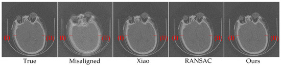
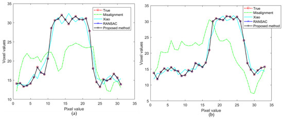
Figure 6.
Comparison of 2D slices after calibration parameter reconstruction under 20% noise.
As seen from Table 3, Xiao et al.’s method and calibration results after RANSAC screening have achieved a certain numerical calibration effect. There are no obvious geometric artifacts in 2D sections of the reconstructed images, as shown in Figure 6. The method detailed in this paper is numerically closer to the true value parameter. The image value of the red line position in Figure 6, displayed in Figure 7. Figure 7a shows the (I) position pixel values with the different corrected methods in Figure 6. Figure 7b shows the pixel values of the (II) position in Figure 6 with different corrected methods. It shows that the calibration result of the proposed method is closer to the calibration result of the true value parameter. This also indicates that the proposed method may have better application in actual data.
3.2. Nanotomography Experimental Section
To verify the proposed method results in the actual data, a nanotomography device developed by the Intelligent Imaging Processing Laboratory in Zhengzhou, Henan Province, China, was used. Scanning parameters: voltage 60 Kv, exposure time 15 s, detector size 1065 pixel × 1030 pixel, pixel size 75 um. A projection was scanned at 3-degree intervals under a circular scan trajectory, and 120 chip-projection data were scanned.
The chip data calibration parameters are shown in Table 4. The calibration result is shown in Figure 8. In the figure, we can see that the three methods all show good correction effects, and the general image information can be recovered well. The method of Xiao et al. still exhibits a slight ghosting phenomenon at the edge of the image. The RANSAC method and the method in this paper produce a clearer edge in the correction results.
Table 4.
The calibration parameters in the Chip data compared with Xiao, RANSAC and our method.
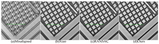
Figure 8.
The Chips data reconstruction results with different parameters. (a) Misaligned parameters. (b) Parameters calculated using Xiao et al.’s method. (c) RANSAC feature-point screening results. (d) Parameters calculated by our proposed method.
The Variance function [25] and the Tenengrad function [26] were also used to evaluate the image quality. The Variance function is a function that evaluates the image sharpness through the image variance, where a clear image has a larger grayscale difference than a blurred image, and the image quality is better. The Tenengrad function is a gradient-based image-sharpness evaluation function where the sharper the edge of the image, the larger the value of the function. The evaluation results are shown in Figure 9b, and we calculate the percentage improvement by averaging the two evaluation functions. Compared with Xiao and RANSAC, it increased by 22.7% and 5.8%, respectively.
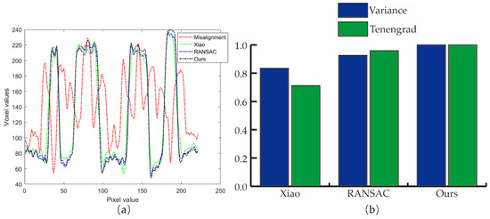
Figure 9.
Graphs showing the numerical analysis results for reconstructed image quality. (a) The green line corresponds to the pixel value; (b) Normalized evaluation results for Variance and Tenengrad.
We also scanned ants in a circular scan trail at 0.25-degree intervals for a total of 1440 slice projection data. Other scanning parameters were the same as chip data. Different methods were used to carry out the contrast experiment of nanotomography system parameter calibration. FDK algorithm is used for 3D reconstruction.
The ant’s data calibration parameters are shown in Table 5. Figure 10 shows the ant data subjected to different methods of calibrating parameters to reconstruct the 2D image slices. All three methods exhibited improved results compared with the uncorrected results, and the blurring and ghosting are suppressed to some extent. The method described in this paper recovers the ant head structure more clearly. The planar maps of two positions in Figure 11 also illustrate the excellent correction results achieved by this method. The results of the two evaluation functions are shown in Figure 11c, which are 25.2% and 14.4% higher than Xiao and RANSAC, respectively. The blurring and ghosting caused by geometric artifacts are significantly suppressed.
Table 5.
Calibration parameters in the Ant data compared with the Xiao, RANSAC and our method.
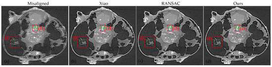
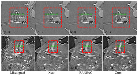
Figure 10.
The Ants data reconstruction results with different parameters. (a) Misaligned parameters. (b) Parameters calculated using Xiao et al.’s method, (c) RANSAC feature-point screening results. (d) Parameters calculated using our proposed method. (a-I–d-I) is an enlarged view of the I position of (a–d). (a-II–d-II) is an enlarged view of the II position of (a–d).
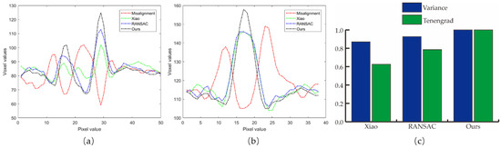
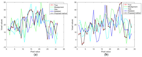
Figure 11.
Graphs showing the numerical analysis results for image quality reconstruction. (a) The pixel value of the green line (I) position inside the red box in Figure 10. (b)The pixel value of the green line (II) position inside the red box in Figure 10. (c) Normalized evaluation results for Variance and Tenengrad.
4. Conclusions
This paper proposes a nanotomography-based geometric parameter self-calibration method based on feature matching of mirror projection images. The method takes full advantage of an image-matching algorithm based on feature points. We design a special feature-point screening algorithm according to the characteristics of the system. This allows some mismatched feature points to be removed and improved accuracy and stability of rotational axis fitting. Simulation and actual data experimental results and numerical analysis prove the effectiveness and practicality of our proposed method. Blurring and ghosting of the reconstructed image caused by geometric artifacts are significantly suppressed. The feature-point-based method exhibits better stability than the self-calibration method that directly constructs the objective function from the gray value of the projected image. In addition, the method utilizes the object’s projection information to achieve correction without the need for additional correction models and iterative reconstruction.
Author Contributions
Conceptualization, S.Y. and Y.H.; methodology, Y.H.; software, S.Y.; validation, S.Y., Y.H., X.X. and L.L.; formal analysis, S.Y. and Y.H.; investigation, S.Y.; resources, B.Y.; data curation, X.X., S.T. and L.Z.; writing—original draft preparation, S.Y. and Y.H.; writing—review and editing, S.T., X.X., L.L. and B.Y.; visualization, S.Y. and M.L.; supervision, B.Y.; project administration, X.X.; funding acquisition, L.L. and Y.H. All authors have read and agreed to the published version of the manuscript.
Funding
This work was supported by the National Key Research and Development Program of China (2020YFC1522002) and the National Natural Science Foundation of China (62201618).
Institutional Review Board Statement
Not applicable.
Informed Consent Statement
Not applicable.
Data Availability Statement
The data and the code used for the manuscript are available for researchers on request from the corresponding author.
Conflicts of Interest
The authors declare no conflict of interest.
References
- Graetz, J.; Müller, D.; Balles, A.; Fella, C. Lenseless X-Ray Nano-Tomography down to 150 Nm Resolution: On the Quantification of Modulation Transfer and Focal Spot of the Lab-Based NtCT System. J. Instrum. 2021, 16, P01034. [Google Scholar] [CrossRef]
- Ferrucci, M.; Leach, R.K.; Giusca, C.; Carmignato, S.; Dewulf, W. Towards Geometrical Calibration of X-Ray Computed Tomography Systems—A Review. Meas. Sci. Technol. 2015, 26, 092003. [Google Scholar] [CrossRef]
- Biguenet, M.; Chaumillon, E.; Sabatier, P.; Paris, R.; Vacher, P.; Feuillet, N. Discriminating between Tsunamis and Tropical Cyclones in the Sedimentary Record Using X-Ray Tomography. Mar. Geol. 2022, 450, 106864. [Google Scholar] [CrossRef]
- Khosravani, M.R.; Reinicke, T. On the Use of X-Ray Computed Tomography in Assessment of 3D-Printed Components. J. Nondestruct. Eval. 2020, 39, 75. [Google Scholar] [CrossRef]
- Noo, F.; Clackdoyle, R.; Mennessier, C.; White, T.A.; Roney, T.J. Analytic Method Based on Identification of Ellipse Parameters for Scanner Calibration in Cone-Beam Tomography. Phys. Med. Biol. 2000, 45, 3489–3508. [Google Scholar] [CrossRef] [PubMed]
- Yang, K.; Kwan, A.L.C.; Miller, D.F.; Boone, J.M. A Geometric Calibration Method for Cone Beam CT Systems: A Geometric Calibration Method for Cone Beam CT. Med. Phys. 2006, 33, 1695–1706. [Google Scholar] [CrossRef] [PubMed]
- Zhao, J.; Hu, X.; Zou, J.; Hu, X. Geometric Parameters Estimation and Calibration in Cone-Beam Micro-CT. Sensors 2015, 15, 22811–22825. [Google Scholar] [CrossRef]
- Yu, J.; Lu, J.; Sun, Y.; Liu, J.; Cheng, K. A Geometric Calibration Approach for an Industrial Cone-Beam CT System Based on a Low-Rank Phantom. Meas. Sci. Technol. 2022, 33, 035401. [Google Scholar] [CrossRef]
- Mayo, S.; Miller, P.; Gao, D.; Sheffield-Parker, J. Software Image Alignment for X-Ray Microtomography with Submicrometre Resolution Using a SEM-Based X-Ray Microscope. J. Microsc. 2007, 228, 257–263. [Google Scholar] [CrossRef]
- Kyriakou, Y.; Lapp, R.M.; Hillebrand, L.; Ertel, D.; Kalender, W.A. Simultaneous Misalignment Correction for Approximate Circular Cone-Beam Computed Tomography. Phys. Med. Biol. 2008, 53, 6267–6289. [Google Scholar] [CrossRef]
- Kingston, A.M.; Sakellariou, A.; Sheppard, A.P.; Varslot, T.K.; Latham, S.J. An Auto-Focus Method for Generating Sharp 3D Tomographic Images. In Developments in X-Ray Tomography VII, Proceedings of the SPIE Optical Engineering + Applications, San Diego, CA, USA, 19 August 2010; Stock, S.R., Ed.; SPIE: Bellingham, WA, USA, 2010; p. 78040J. [Google Scholar]
- Tan, S.; Cong, P.; Liu, X.; Wu, Z. An Interval Subdividing Based Method for Geometric Calibration of Cone-Beam CT. NDT E Int. 2013, 58, 49–55. [Google Scholar] [CrossRef]
- Yang, X.; De Carlo, F.; Phatak, C.; Gürsoy, D. A Convolutional Neural Network Approach to Calibrating the Rotation Axis for X-Ray Computed Tomography. J. Synchrotron Radiat. 2017, 24, 469–475. [Google Scholar] [CrossRef] [PubMed]
- Xiao, K.; Yan, B. Correction of Geometric Artifact in Cone-Beam Computed Tomography through a Deep Neural Network. Appl. Opt. 2021, 60, 1843. [Google Scholar] [CrossRef] [PubMed]
- Panetta, D.; Belcari, N.; Del Guerra, A.; Moehrs, S. An Optimization-Based Method for Geometrical Calibration in Cone-Beam CT without Dedicated Phantoms. Phys. Med. Biol. 2008, 53, 3841–3861. [Google Scholar] [CrossRef] [PubMed]
- Patel, V.; Chityala, R.N.; Hoffmann, K.R.; Ionita, C.N.; Bednarek, D.R.; Rudin, S. Self-Calibration of a Cone-Beam Micro-CT System: Self-Calibration of a Cone-Beam Micro-CT System. Med. Phys. 2008, 36, 48–58. [Google Scholar] [CrossRef]
- Meng, Y.; Gong, H.; Yang, X. Online Geometric Calibration of Cone-Beam Computed Tomography for Arbitrary Imaging Objects. IEEE Trans. Med. Imaging 2013, 32, 278–288. [Google Scholar] [CrossRef]
- Xiao, K.; Han, Y.; Xi, X.; Yan, B.; Bu, H.; Li, L. A Parameter Division Based Method for the Geometrical Calibration of X-Ray Industrial Cone-Beam CT. IEEE Access 2018, 6, 48970–48977. [Google Scholar] [CrossRef]
- Lin, Q.; Yang, M.; Meng, F.; Sun, L.; Tang, B. Calibration Method of Center of Rotation under the Displaced Detector Scanning for Industrial CT. Nucl. Instrum. Methods Phys. Res. Sect. A Accel. Spectrometers Detect. Assoc. Equip. 2019, 922, 326–335. [Google Scholar] [CrossRef]
- Torr, P.H.S.; Zisserman, A. MLESAC: A New Robust Estimator with Application to Estimating Image Geometry. Comput. Vis. Image Underst. 2000, 78, 138–156. [Google Scholar] [CrossRef]
- Xu, J.; Tsui, B.M.W. A Graphical Method for Determining the In-Plane Rotation Angle in Geometric Calibration of Circular Cone-Beam CT Systems. IEEE Trans. Med. Imaging 2012, 31, 825–833. [Google Scholar] [CrossRef]
- Ferrucci, M.; Ametova, E.; Carmignato, S.; Dewulf, W. Evaluating the Effects of Detector Angular Misalignments on Simulated Computed Tomography Data. Precis. Eng. 2016, 45, 230–241. [Google Scholar] [CrossRef]
- Zhang, N. Computing Optimised Parallel Speeded-Up Robust Features (P-SURF) on Multi-Core Processors. Int. J. Parallel Program. 2010, 38, 138–158. [Google Scholar] [CrossRef]
- Muja, M.; Lowe, D.G. Scalable Nearest Neighbor Algorithms for High Dimensional Data. IEEE Trans. Pattern Anal. Mach. Intell. 2014, 36, 2227–2240. [Google Scholar] [CrossRef] [PubMed]
- Aja-Fernandez, S.; Estepar RS, J.; Alberola-Lopez, C.; Westin, C.F. Image quality assessment based on local variance. In Proceedings of the 2006 International Conference of the IEEE Engineering in Medicine and Biology Society, New York, NY, USA, 30 August–3 September 2006; IEEE: Pasadena, NJ, USA, 2006; pp. 4815–4818. [Google Scholar]
- Yeo TT, E.; Ong, S.H.; Sinniah, R. Autofocusing for tissue microscopy. Image Vis. Comput. 1993, 11, 629–639. [Google Scholar]
Publisher’s Note: MDPI stays neutral with regard to jurisdictional claims in published maps and institutional affiliations. |
© 2022 by the authors. Licensee MDPI, Basel, Switzerland. This article is an open access article distributed under the terms and conditions of the Creative Commons Attribution (CC BY) license (https://creativecommons.org/licenses/by/4.0/).