Article

Assessing Database Contribution via Distributed Tracing for Microservice Systems

1
Beijing Institute of Computer Technology and Application, Beijing 100854, China
2
School of Computer Science and Technology, Xidian University, Xi’an 710071, China
3
College of Systems Engineering, National University of Defense Technology, Changsha 410073, China
*
Author to whom correspondence should be addressed.
Appl. Sci. 2022, 12(22), 11488; https://doi.org/10.3390/app122211488
Submission received: 20 September 2022 / Revised: 26 October 2022 / Accepted: 8 November 2022 / Published: 12 November 2022

Abstract

:
Microservice architecture is the latest trend in software systems development and transformation. In microservice systems, databases are deployed in corresponding services. To better optimize runtime deployment and improve system stability, system administrators need to know the contributions of databases in the system. For the high dynamism and complexity of microservice systems, distributed tracing can be introduced to observe the behavior of business scenarios on databases. However, it is challenging to evaluate the database contribution by combining the importance weight of business scenarios with their behaviors on databases. To solve this problem, we propose a business-scenario-oriented database contribution assessment approach (DBCAMS) via distributed tracing, which consists of three steps: (1) determining the importance weight of business scenarios in microservice system by analytic hierarchy process (AHP); (2) reproducing business scenarios and aggregating the same operations on the same database via distributed tracing; (3) calculating database contribution by formalizing the task as a nonlinear programming problem based on the defined operators and solving it. To the best of our knowledge, our work is the first research to study this issue. The results of a series of experiments on two open-source benchmark microservice systems show the effectiveness and rationality of our proposed method.

1. Introduction

Microservice architecture [1] is an architectural style and approach that develops a single large and complex application as a series of small services, each running in its own process and communicating with lightweight mechanisms such as HTTP APIs. The application system based on microservice architecture (referred to as microservice systems hereafter) has the advantages of independent development, easy continuous delivery, maintenance, scalability, and autonomy compared with monolithic applications [1,2,3,4]. Therefore, in recent years, microservice architecture has become the mainstream for cloud-native application systems, and more and more companies or organizations have chosen to transform their application systems from traditional monolithic architecture to microservice architecture [5,6].
However, software systems adopting microservice architecture have inherent problems, i.e., the highly dynamic and complex environment at runtime, making it more difficult to understand, diagnose, and debug than monolithic software [3]. Specifically, microservice systems usually contain many business scenarios, and related databases that support these business scenarios are deployed in corresponding different services. Each business scenario contains a series of business requests, and the execution of a request usually involves a complex service call chain possessing a large number of service interactions [7], where each service in the call chain records logs respectively. In addition, asynchronous or multithreaded calls also widely exist in microservice systems. These factors make it tough to obtain the support information of the databases for business scenarios by analyzing the log sequence similar to monolithic applications [8,9]. However, in the process of running and maintaining a microservice system, the support information of databases is important for operation engineers and developers.
We define the support of databases to the business scenarios as the contribution of databases, and the task of this paper is to study how to assess the contributions of business-related databases to upper-level business scenarios in microservice systems. As far as we know, there is little previous research on assessing database contribution in microservice systems, but it is meaningful and valuable to study this issue from the perspective of runtime deployment optimization and system stability. Specifically, for example, in the scene where the resources of cluster are relatively sufficient, appropriately increasing the number of instances of services where the databases with high contribution are located can reduce the average response time of businesses to a certain extent [10]. In addition, it can perform multiservice hot standby operations on services hosted by databases with high contribution to improve the stability of the entire application [11].
In order to evaluate the contributions of databases to business scenarios in the microservice system, for the dynamic and complex features of the microservice system mentioned above, distributed tracing [12] can be introduced to observe the invocations between the services, which include behavior information on the database (tables). At the same time, business scenarios in a system always have different importance weight [13] (for example, for an online shopping store, purchasing goods is more important than viewing historical orders). The challenge of this study is determining how to consider both the importance weight of business scenarios and their operations on databases in assessing database contribution.
In this paper, we propose a business-scenario-oriented database contribution assessment approach via distributed tracing for microservice systems. First, the importance weight of the main business scenarios of the microservice system is determined by the analytic hierarchy process (AHP) [14]. Second, we reproduce the business scenarios of the system. At the same time, based on the traces obtained by distributed tracing, for each business scenario, the numbers of records with the same operation on the same database are aggregated. Finally, we define operators for four basic database operations (creating, retrieving, updating and deleting) to formalize the task of database contribution assessment as a nonlinear programming problem. By solving this nonlinear programming problem, the contributions of databases in the microservice system can be gained. It should be noted that each database in the system could contain one or more tables, and the granularity of our method is the database. Our main contributions are summarized as follows:
  • To the best of our knowledge, this paper is the first research to assess the contributions of the databases to business scenarios for microservice systems based on the information observed by distributed tracing.
  • The method proposed in this paper considers the importance weight of business scenarios and defines operators for the four basic database operations (creating, retrieving, updating, and deleting) so as to skillfully formulate this task as a nonlinear programming problem.
  • The experimental results on two open-source benchmark microservice systems (i.e., Sock-Shop [15] and TrainTicket [16]) demonstrate the effectiveness and rationality of our proposed method.
The rest of this paper is structured as follows. Section 2 introduces the related work about distributed tracing and contribution assessment. Section 3 defines the task and details our proposed method. Section 4 introduces the experimental settings and analyzes the experimental results in detail. Section 5 discusses some issues about the method and experiments in this paper. Section 6 provides the conclusion and future work of our study.

2. Related Work

This work is based on the information obtained from distributed tracing to assess the contributions of databases in microservice systems. Hence, related work is divided into two categories: the background, basic concepts, and related research and applications of distributed tracing; and the related research of contribution assessment.

2.1. Distributed Tracing

Due to the complexity, dynamics, and uncertainty at runtime, it becomes more difficult to understand, diagnose, and debug the microservice system [4]. Therefore, observability [17] is regarded as the basic requirement of microservice systems. As a significant means to achieve observability, distributed tracing has been widely accepted and practiced in the industry. According to the industrial research in [12], distributed tracing is mainly used in timeline analysis, service dependency analysis, aggregation analysis, root cause analysis, and anomaly detection for microservice systems. Google introduced the first distributed tracing system, Dapper [18], in 2010, which led to the rapid development of distributed tracing. In recent years, many active distributed tracing projects in the open-source community, such as Pinpoint [19], Zipkin [20], Jaeger [21], and SkyWalking [22], have followed fundamental principles and working mechanisms of Dapper. At the same time, specifications such as OpenTracing [23], OpenCensus [24], and OpenTelemetry [25] have been formulated within the industry.
The data model adopted by the OpenTracing specification, shown in Figure 1, mainly involves two core concepts:
  • Span: A call between two services or threads is called a span. Several properties are recorded in the span, including the operation name, start and end timestamps, span tags, span logs, span context, etc.
  • Trace: A directed acyclic graph composed of multiple spans is called a trace.
For a specific system, a trace represents a complete process of processing business requests; a span represents a specific call in this business request. A request generates a unique trace ID and propagates throughout the trace, i.e., spans belonging to the same trace have the same trace ID. At the same time, each span also has a unique span ID; except for the outermost span, each span has a span as its own parent and is marked with parent ID. In addition, span context is the information transmitted in the trace along with distributed transactions. It generally records two parts: one is the data necessary to implement the trace, such as the trace ID, the span ID, and the data required by downstream services; the other is the user-defined data recorded as key-value pairs for subsequent analysis.
At the same time, a lot of research has been conducted based on distributed tracing. Zhou et al. [26] proposed an approach, named MEPFL, of latent error prediction and fault localization for microservice applications by learning from system trace logs. Guo et al. [3] proposed a graph-based approach of microservice trace analysis, named GMTA, for understanding architecture and diagnosing various problems, which includes efficient processing of traces produced on the fly and has been implemented and deployed in eBay. Zhang et al. [9] proposed a deep-learning-based microservice anomaly detection approach named DeepTraLog, which uses a unified graph representation to describe the structure of a trace, and trains models by combining traces and logs. In [27], with their novel trace representation and the design of deep Bayesian networks with posterior flow, Liu et al. designed an unsupervised anomaly detection system called TraceAnomaly, which can accurately and robustly detect trace anomalies in a unified fashion. Bogner et al. [28] designed an approach to calculate service-based maintainability metrics from runtime data and implemented a prototype with a Zipkin integrator.

2.2. Contribution Assessment

Since there are few studies on the evaluation of database contribution, we introduce the research on contribution assessment in other fields.
Node importance ranking in complex networks has received more and more attention in recent years because of its great theoretical and application value. Common methods for identifying and evaluating vital nodes in a network can be classified into structural centralities (including neighborhood-based centralities [29,30,31] and path-based centralities [32,33,34]), iterative refinement centralities [35,36,37,38,39], node operation [40], and dynamics-sensitive methods [41]. Among them, PageRank [36] is a famous variant of eigenvector centrality and is used to rank websites in the Google search engine and other commercial scenarios. LeaderRank [37] later improved two problematic issues in PageRank.
For the evaluation of developers’ contributions in open-source projects, Gousios et al. [42] proposed a model that, by combining traditional contribution metrics with data mined from software repositories, can deliver accurate developer contribution measurements; Zhou et al. [43] suggested researching the contributions of developers from three aspects: motivation, capability, and environment.
To enable fair credits allocation for each party in federated machine learning (FML), Wang et al. [44] developed techniques to fairly calculate the contributions of multiple parties in FML, in the context of both horizontal FML and vertical FML. Boyer et al. [45] proposed an easy-to-apply, universally comparable, and fair metric named Author Contribution Index (ACI) to measure and report co-authors’ contributions in the scientific literature, and ACI is based on contribution percentages provided by the authors.

3. Methodology

3.1. Problem Definition

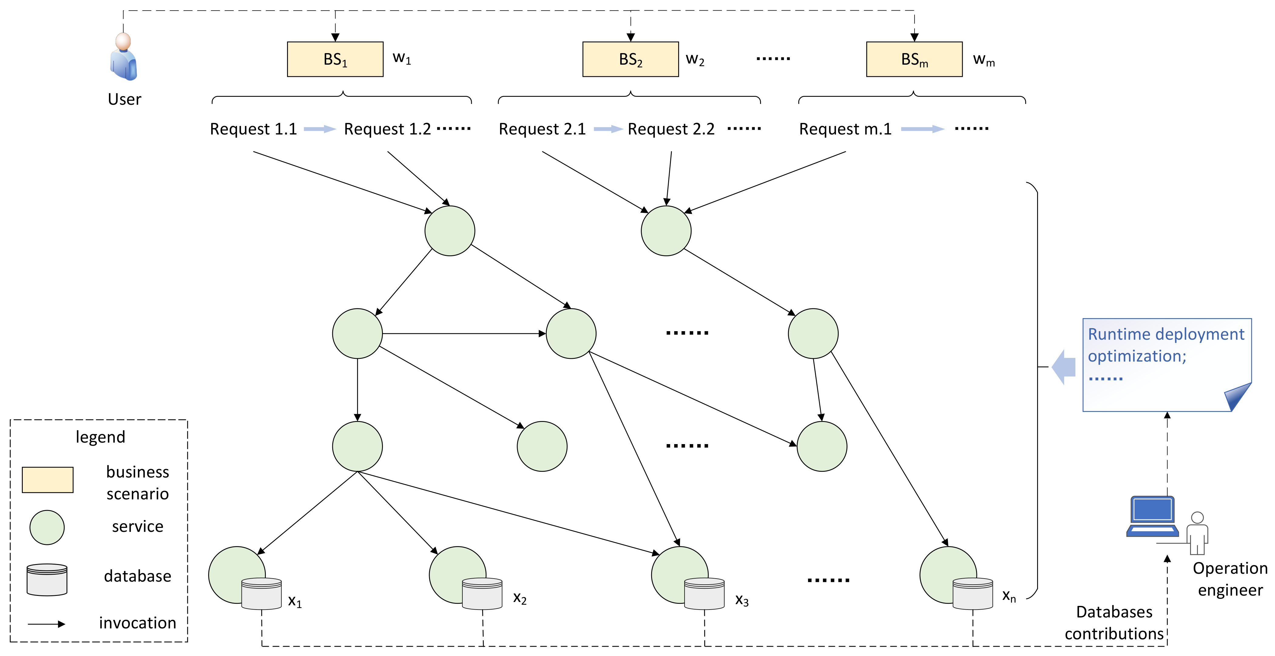
As shown in Figure 2, given a microservice system MS = ( B S , D B ) , where B S = ( B S 1 , , B S m ) represents m-number business scenarios, and D B = ( D B 1 , , D B n ) represents n-number business-related databases deployed in the system, we denote the importance weight vector of business scenarios as w = ( w 1 , , w m ) . The task of this paper is to calculate the vector x = ( x 1 , , x n ) , i.e., the contributions of n-number databases to m-number business scenarios. The invocations in Figure 2 are obtained by distributed tracing, which contains the behavioral information of the business scenarios on the databases.

3.2. Method Framework

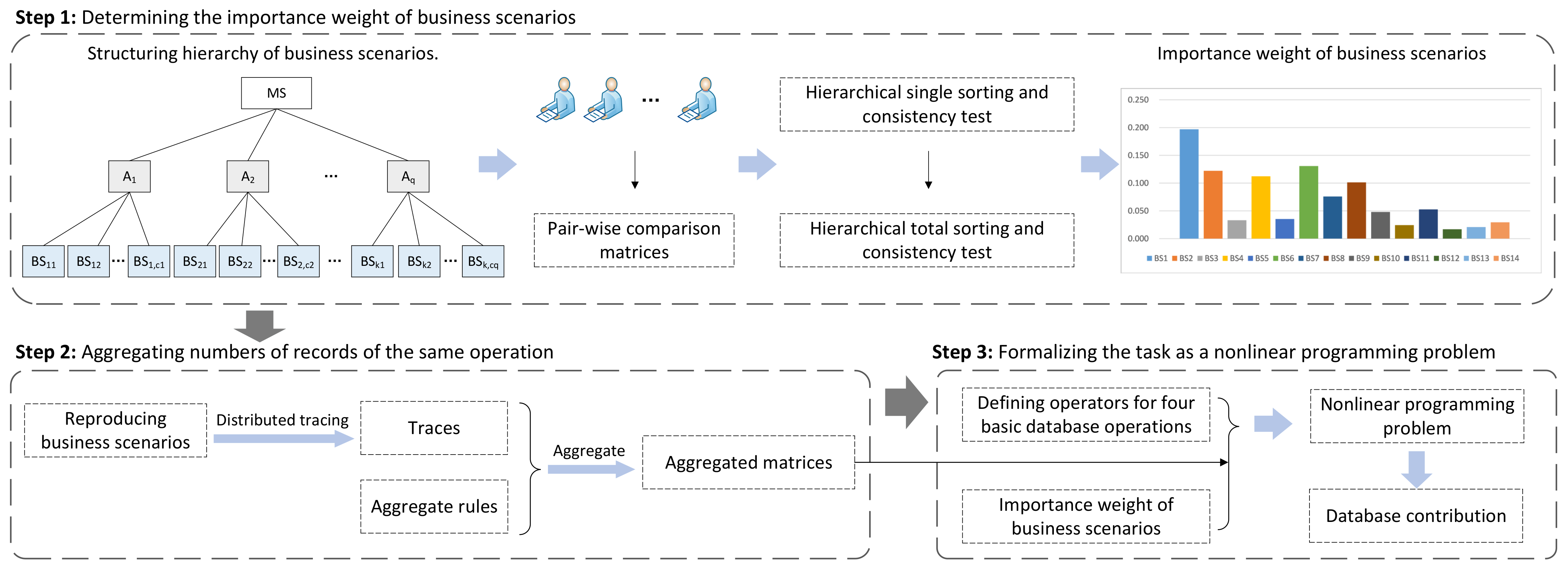
We propose a business-scenario-oriented database contribution assessment approach, and the framework is illustrated in Figure 3. First, the importance weight of business scenarios is determined by AHP, which includes constructing a business scenarios hierarchy, generating pairwise comparison matrices, hierarchical sorting, and consistency test. Second, we reproduce business scenarios, and the corresponding traces are generated by distributed tracing, which contain behavioral information about databases in span tags or span logs. At the same time, according to each business scenario and aggregate rules, the numbers of records with the same operation on the same database are aggregated. Third, we define operators for four basic database operations (creating, retrieving, updating, and deleting). Meanwhile, based on the business scenarios’ importance weight and the aggregated matrices obtained in the second step, the database contribution assessment is formalized as a nonlinear programming problem, which some corresponding optimization algorithms or tools can solve.

3.3. Determining the Importance Weight of Business Scenarios

We determine the importance weight of the m-number business scenarios through analytical hierarchy process (AHP) [14,46]. AHP is a multicriteria decision-making approach, which was proposed by American operations research scientist Saaty in the 1970s. It has been widely used in enterprise management, engineering scheme determination, resource allocations, resolving conflict, etc. [47]. For determining the importance weight of business scenarios, the four steps are as follows:
Step 1. Structuring hierarchy of business scenarios.
By combiningthe business scenarios of the microservice system, a hierarchical structure can be built, including the top layer, the middle layer (m-number business scenarios are divided into q-number different categories, and there are c i -number business scenarios in the i-th category, i.e., c 1 + c 2 + + c q = m ; in simple systems, this layer can be omitted), and the bottom layer (m-number business scenarios layer), as shown in Figure 4. It is important to note that the business scenarios cover at least all major business processes and functions.
Step 2. Constructing pairwise comparison matrices.
Construct a set of pairwise comparison matrices for each of the lower levels with one matrix for each element in the level immediately above. For example, for the hierarchy model in Figure 4, a total of q + 1 pairwise comparison matrices need to be constructed. This step is usually achieved by inviting experts in related fields to use the relative scale measurement shown in Table 1 [14,46] for scoring. Denote the pairwise comparison matrix as C , and c i j represents the comparison result of the i-th element relative to the j-th element (the orders of the q + 1 pairwise comparison matrices for the hierarchy model in Figure 4 are q , c 1 , c 2 , , c q , respectively).
Step 3. Hierarchical single sorting and consistency test.
Hierarchical single ordering refers to calculating the importance weight of the elements in the lower layer to the corresponding element of the upper immediately layer. Correspondingly, for the hierarchy shown in Figure 4, we need to execute hierarchical single sorting and consistency test q + 1 times, and we illustrate this process using the middle layer (BS categories layer) as an example. Generally, hierarchical single sorting can be solved by the eigenvector method [48], as is shown in Equation (1).
C MS w ^ = λ m a x w ^
where C MS is the corresponding q-order pairwise comparison matrix, λ m a x is the largest eigenvalue of it, and w ^ is the corresponding eigenvector of λ m a x . According to the properties of the pairwise comparison matrix [48], λ m a x exists and is unique, the components of w ^ are all positive components, and normalized w ^ is the result of hierarchical single sorting. However, whether the calculated results are acceptable or not requires a consistency test, which requires the following two steps.
  • Calculating consistency index (CI).
    CI is determined by using the eigenvalue, as is illustrated in Equation (2).
    C I = λ m a x q q 1
    where q is the order of the pairwise comparison matrix C M S .
  • Calculating consistency ratio (CR).
    C R = C I R I
    If q > 2, to measure the size of CI, the average random consistency index (RI) is introduced. RI under different matrix size is provided in Table 2 [14,46], which was calculated by Saaty as the average consistency of square matrices of various orders n filled with random entries. If the CR is less than 0.1, it is considered that the pairwise comparison matrix is nearly consistent, i.e., the corresponding hierarchical single sorting result is accepted; otherwise, the pairwise comparison matrix C M S should be reviewed and improved.
Step 4. Hierarchical total sorting and consistency test.
Hierarchical total sorting refers to calculating the relative importance of all elements from a certain level to the top level. Calculating a hierarchical total sorting requires knowing the hierarchical total sorting of its upper elements, which is a top-down calculation process. For the hierarchy model in Figure 4, denote the hierarchical total sorting result of the middle layer as a 1 , a 2 , , a q , and denote the hierarchical single sorting result of the bottom layer as b 1 , b 2 , , b m , then the hierarchical total sorting of the i-th business scenario (assume it belongs to the j-th category) is
w i = a j · b i
where 1 i m , 1 j q .
Similarly, a consistency test is required to ensure that the hierarchical total sorting result is acceptable. For the hierarchy model in Figure 4, denote the hierarchical single sorting consistency index of the B S layer to the elements A i ( i = 1 , 2 , . . . , q ) in the upper layer as C I i , and the average random consistency as R I i , then the consistency ratio of the hierarchical total sorting can be calculated by Equation (5).
C R _ t o t a l = i = 1 q a i · C I i i = 1 q a i · R I i
If C R _ t o t a l < 0.1, the hierarchical total sorting result is acceptable, and the bottom element importance vector w = ( w 1 , , w m ) can be obtained; otherwise, the pairwise comparison matrices with a higher consistency ratio need to be adjusted. When multiple experts participate in scoring, the final result can be obtained by averaging the hierarchical total sorting results of all experts.

3.4. Aggregating Numbers of Records of the Same Operation

The method in this paper is oriented to business scenarios. Therefore, to reproduce a business scenario, a typical business process that contains a series of interface inputs or clicks can be executed automatically or manually. At the same time, we use a distributed tracing tool to generate corresponding traces which contain behavioral information on the database table in span tags or span logs. For example, from the span tags in Table 3, we can see the query operation of the current span on the Catalogue table.
Then, for each business scenario, we aggregate numbers of records based on the following rules:
  • It aggregates the numbers of records of the same operation on the same database. When a database contains multiple tables, the aggregation result can be obtained by counting the number of records of the same operation for each table.
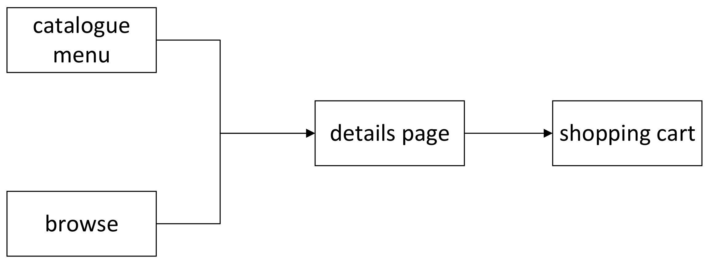
  • For parallel behavior in the typical process of business scenarios, the average value of the numbers of the records of the same operation on the same database of them is adopted. For example, as illustrated in Figure 5, there are three steps in a typical process of purchasing socks and two parallel behaviors (i.e., catalogue menu and browse) in the first step. Assume that the numbers of records of retrieving operations on the Catalogue for catalogue menu, browse, and detail page are r c , r b , and r d , respectively, and the third step does not have a retrieving operation on the Catalogue. Then, for Purchasing socks, the aggregated result of the number of records of retrieving operations on the Catalogue is r c + r b 2 + r d .
Finally, for the i-th business scenario, an aggregation matrix AM i i = 1 , 2 , , m can be obtained based on the above rules:
AM i = c i 1 r i 1 u i 1 d i 1 c i 2 r i 2 u i 2 d i 2 c i n r i n u i n d i n n × 4
where n denotes the number of databases in the microservice system; c i k , r i k , u i k , and d i k , respectively, represent the number of records required to create, retrieve, update, and delete on the k-th 1 k n database to complete the i-th business scenario.

3.5. Formalizing the Task as a Nonlinear Programming Problem

To transform this problem into a mathematical problem, we define corresponding operators for the four basic operations on the database (creating, retrieving, updating, and deleting), as shown in Table 4.
In our definition, α , β , γ , and δ are four parameters, representing the weight of creating, retrieving, updating, and deleting operations, respectively. Based on the aggregated matrices of business scenarios, the number of records processed by each operation can be calculated by the equations in Table 5. The weight of the operation corresponding to the smallest number of records is 1; the weight of the operation corresponding to the smaller number of records is 2; the weight of the operation corresponding to the larger number of records is 3; the weight of the operation corresponding to the largest number of records is 4.
N i in the operators represents the numbers of operated records in the i-th business scenario, which can be calculated by Equation (7).
N i = k = 1 n c i k + r i k + u i k + d i k
The structure of the defined operators in Table 4 can ensure that the number of operated records h and the weight of four basic database operations maintain a positive correlation with database contribution x k , to a certain extent, while appropriately reducing the impact of the large gap between h on the calculating database contribution.
Based on the defined operators and the aggregation matrix of each business scenario, we can use the database contribution x 1 , x 2 , , x n to represent the importance weight vector g = ( g 1 , g 2 , , g m ) of business scenarios:
g i = k = 1 n 1 c i k N i α + r i k N i β + u i k N i γ + d i k N i δ x k
Then, combined with the business scenario importance weight w by AHP, the database contribution assessment problem can be formalized as the following nonlinear programming problem:
M i n 1 g · w g · w 2 s . t . i = 1 n x i = 1 , x i 0 , 1 , i = 1 , 2 , , n
The optimization objective in Equation (9) is defined based on cosine similarity. According to the meaning of cosine similarity, Equation (9) essentially finds the x that minimizes the angle between vector g and vector w under constraints, which is a constrained nonlinear optimization problem.
For the above nonlinear optimization problem, there are generally two kinds of solutions: traditional mathematical analysis-based methods (such as sequential quadratic programming) and heuristic algorithms (such as genetic algorithm and simulated annealing). Traditional methods usually depend on the initial value of the function and the gradient information, and easily fall into local optimum. However, the heuristic algorithm does not depend on the mathematical properties of the problem itself, has better adaptability, and more easily obtains the optimal solution [49]. Therefore, we use the classic heuristic algorithm, genetic algorithm, to optimize Equation (9).

4. Experiments

In this section, we conduct experiments on two open-source benchmark microservice systems to verify the effectiveness and rationality of the method proposed in this paper. Two microservice systems are deployed by Docker. Each service has one instance, and Docker-compose is used to orchestrate the docker containers cluster. The databases of both systems are deployed in their respective database services, and each database contains only one table (the database has the same name as the table). Additionally, there is no special requirement for setting the size of database tables, as long as it is able to run the typical business process of a corresponding business scenario.

4.1. Experimental Systems and Settings

4.1.1. Sock-Shop

Sock-Shop [15] is a small typical microservice application containing 13 services for online selling. Services in Sock-Shop are implemented in multiple languages (e.g., Java, .NET, and Go). The entire application is divided into services with a single function that can be independently developed, deployed, and extended. Sock-Shop has been widely used in microservice research [26,50,51]. It fully implements the primary online shopping businesses, and related business databases are deployed in the system. Therefore, this paper uses Sock-Shop as the experimental object.
Four databases (i.e., User, Order, Catalogue, and Cart) in the system and their descriptions and numbers of records are shown in Table 6.
In the system, there are three users, and each user has five records in the shopping cart and ten historical orders; at the same time, there are nine pairs of socks belonging to different categories.

4.1.2. TrainTicket

To verify the applicability of this method to larger-scale microservice systems, we conduct a study on the V0.2.0 of TrainTicket [16]. TrainTicket is a medium-scale open-source microservice system for train ticket booking that provides typical functions, including ticket query, reservation, rebooking, order management, etc. It contains 45 business services written in different languages (e.g., Java, JavaScript, Python), as well as basic services such as messaging middleware services, distributed caching services, and database services. The total number of services is over 70, and services communicate with synchronous REST calls and asynchronous messaging.
Sixteen business-related databases to be evaluated in the system and their descriptions and numbers of records are shown in Table 7.
In the experiment, we registered twenty users; each user reserved twenty tickets, had an average of four pieces of consignment information, and had four contacts. Ten routes containing thirteen stations and ten corresponding travels are set in the system, including five high-speed trains (GaoTie/DongChe) and five ordinary trains, as well as the price ratio information of the corresponding ten travels. Five high-speed trains (GaoTie/DongChe) correspond to five pieces of train food information; the Food-map contains information about six restaurants. The system also contains a piece of configuration named DirectTicketAllocationProportion. In addition, since high-speed trains and ordinary trains have almost the same business logic, we calculate the contributions of their respective related databases (i.e., Order and Travel) uniformly.

4.2. Baseline Methods

To verify the effectiveness of DBCAMS, we choose the following two baselines for comparison.
  • DBCAMS-MMD: Replace maximizing cosine similarity with minimizing maximum mean discrepancy [52] (MMD) in DBCAMS. MMD can be used to test the similarity between the two distributions. When MMD becomes smaller, the two distributions become more similar.
  • DBCAMS-RN: Remove the N i of the defined operator in DBCAMS. For example, the operator of “Create h records on the k-th database in the i-th business scenario.” changes from 1 h N i α x k to 1 h α x k , and the rest is the same as DBCAMS.
The three methods (DBCAMS and two baselines) correspond to three different optimization objectives, all of which are solved by genetic algorithm. To compare the optimization effects of them, we select L2-Norm g g 1 w w 1 as the index. The method with a smaller L2-Norm has a better optimization effect.

4.3. Main Results

In this section, we present and analyze the main results according to the steps of our method described in Section 3.

4.3.1. Sock-Shop

Step 1. Determining the importance weight of business scenarios.
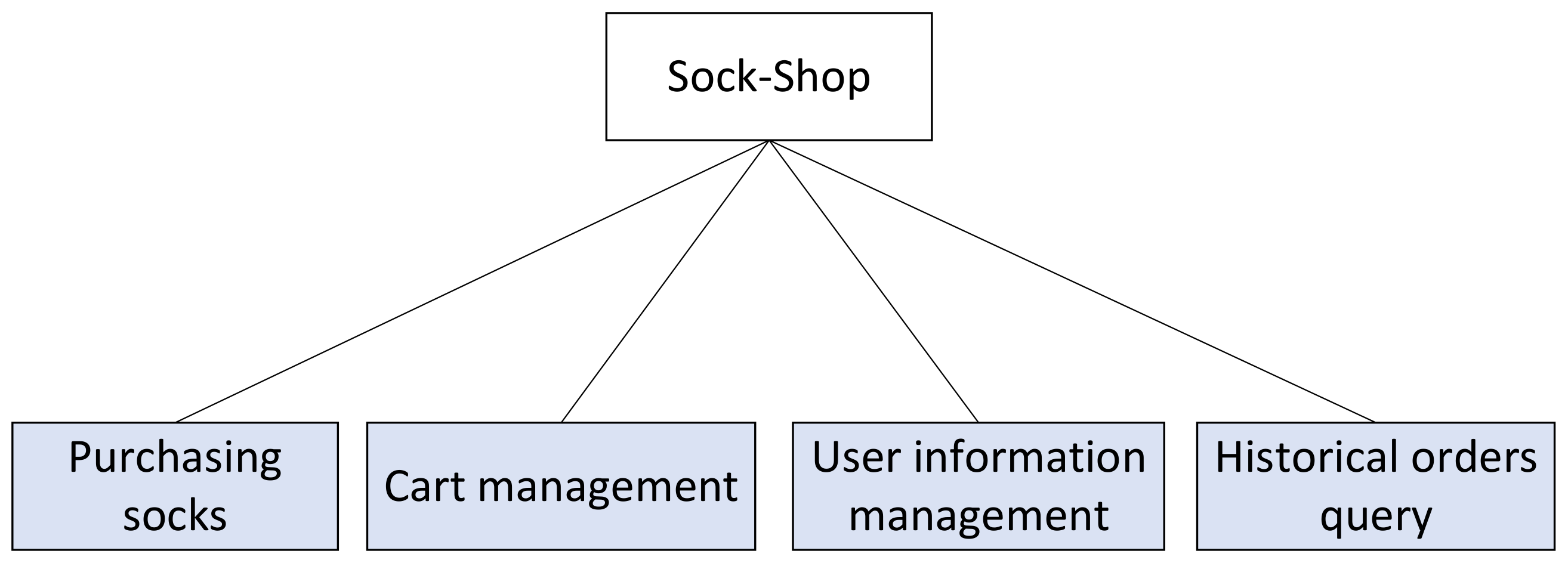
By analyzing the main functions and processes of Sock-Shop, the hierarchy structure is illustrated in Figure 6.
Then, we invited five related experts to score the business scenarios, and the pairwise comparison matrices are shown in Appendix A (Table A1, Table A2, Table A3, Table A4 and Table A5). By hierarchical sorting and consistency test (Table A6 in Appendix A), the final importance weight of business scenarios in Sock-Shop can be calculated and are shown in Table 8.
Step 2. Aggregating numbers of records of the same operation.
Since aggregation matrices are sparse, we present the aggregation results of business scenarios in Sock-Shop in tabular form (Table 9).
Step 3. Calculating database contribution.
By solving the three corresponding nonlinear programming problems (using the genetic algorithm in the MATLAB global optimization toolbox), the optimization results are shown in Table 10. The L2-Norm of DBCAMS is 0.1456, which is better than the other two baseline methods.
The difference in optimization effects between DSCAMS and DBCAMS-MMD is caused by the difference between maximizing cosine similarity and minimizing MMD. Cosine similarity measures the consistency of the direction between vector dimensions, and pays more attention to the differences between dimensions than the differences in numerical values; MMD maps the two samples to be compared into a high-dimensional space (Reproducing Kernel Hilbert Space, RKHS) through a kernel function to find the distance between the two samples in RKHS. The reason for the better performance of DBCAMS is probably that w and g are more suitable for directional optimization in this situation; when the samples are mapped from low to high dimensions, the large dimension gap may cause noise generation.
The difference in optimization effects between DSCAMS and DBCAMS-RN is caused by difference between the operators. The role of N i is to reduce the influence of the gap between the number of operation records on calculating contribution, which not only ensures the positive correlation between the number of operation records and the database contribution, but also reduces the error in the optimization process.
Meanwhile, according to the result from DBCAMS, Catalogue has the highest contribution (close to 0.5), mainly because the importance of Purchasing socks is high, and the invocations to Catalogue account for a high proportion in Purchasing socks. The contributions of the Cart and User are close (both are about 0.25). The Order has the lowest contribution, mainly because the importance of the Historical order query is low (only 0.0769), and this business scenario only calls the Order.

4.3.2. TrainTicket

Step 1. Determining the importance weight of business scenarios.
By combiningand analyzing the business scenarios of TrainTicket, a three-tier hierarchy structure is built in Figure 7.
According to the hierarchy model in Figure 7, we invited five experts familiar with the business to score. At the same time, it is agreed that the user catalogue and the administrator catalogue are of the same importance to the system, i.e., the experts only need to construct pairwise comparison matrices for the third layer of the hierarchy. The pairwise comparison matrices for user business scenarios ( User _ C i , i = 1 , 2 , , 5 ) and administrator business scenarios ( Admin _ C i , i = 1 , 2 , , 5 ) are shown in Appendix B (Table A8, Table A9, Table A10, Table A11, Table A12, Table A13, Table A14, Table A15, Table A16 and Table A17). Table 11 presents the final importance weights of business scenarios obtained through hierarchical sorting and consistency tests (Table A18, Table A19 and Table A20 in Appendix B).
Step 2. Aggregating numbers of records of the same operation.
Similarly, since aggregation matrices are sparse, we present the aggregation results in Table 12.
Step 3. Calculating database contribution.
By solving the three corresponding nonlinear programming problems (using the genetic algorithm in the MATLAB global optimization toolbox), the optimization results are shown in Table 13. DBCAMS has better optimization results (the L2-Norm is 0.3558) than others. Similar reasons are analyzed in the main results of Sock-Shop.
According to the result from DBCAMS, Route, Travel, Station, and Order have higher contributions, and the contributions of other databases are between 0.02 and 0.05. Route and Station contribute more because both databases are invoked and account for higher proportions of operated records in Ticket reserve, User/Admin order management, and Advanced search business scenarios. The low contribution of other databases is mainly due to the low importance of the primary business scenarios in which they are invoked (Consign, User, and Contact). The number of records operated in related business scenarios is small (Assurance, Security, Train-food, Consign-price, and Food-map); other databases belonging to the same business scenarios have high contributions (Config and Train).

4.4. Results Analysis of Different Optimization Algorithms

In this section, we analyze the optimization effect of Equation (9) with different algorithms and L2-Norm g g 1 w w 1 as the evaluation index. For traditional methods, we choose interior point method and sequential quadratic programming (SQP) for comparison; for heuristic algorithm, we choose particle swarm optimization (PSO) and simulated annealing algorithm (SA) for comparison.
From the results in Table 14, we can see that for a single system, the optimization effect between traditional algorithms is basically the same, and the optimization effect between heuristic algorithms is basically the same, but the heuristic algorithms are generally better than the traditional methods.

4.5. The Impact of Business Scenarios’ Importance Weight

In this section, we analyze the impact of business scenarios’ importance on database contribution through experiments on the two systems based on DBCAMS. Based on the aggregation matrix AM i ( i = 1 , 2 , , m ) of each business scenario in the microservice system, we can calculate the sum of the number of records processed by the four basic operations (creating, retrieving, updating, and deleting) on each database s k k = 1 , 2 , , n by Equation (10).
s k = i = 1 m c i k + r i k + u i k + d i k
As mentioned above, the database contribution is positively related to the number of records operated on it. Next, we analyze the experimental results of the two systems in detail.

4.5.1. Sock-Shop

Based on Table 9 and Equation (10), the total numbers of records operated on databases and corresponding contribution ranking in the Sock-Shop are shown in Table 15.
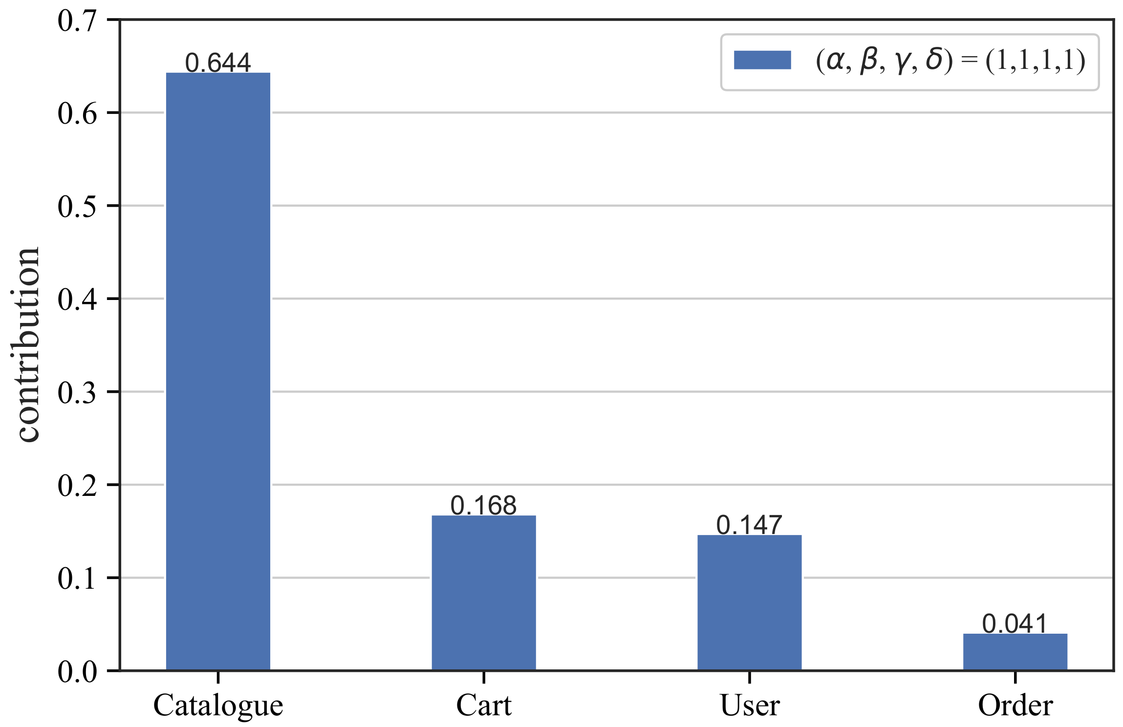
When considering business scenarios’ weight (Table 8), the database contributions are shown in Figure 8 (assuming that the four basic operations have the same importance, i.e., α = β = γ = δ = 1 ). At this time, Catalogue, Cart, User, and Order are ranked from high to low in the order of database contribution. The main reason is that although the Order has the most records to be operated, the Historical order query is the least important, and it only calls the Order. At the same time, although the Catalogue has the lowest number of records to be operated, the Purchasing socks has the highest importance, and the Catalogue has a higher proportion of operational records in this business scenario.

4.5.2. TrainTicket

Based on Table 12 and Equation (10), the total numbers of records operated on databases and corresponding contribution ranking in the TrainTicket are shown in Table 16.
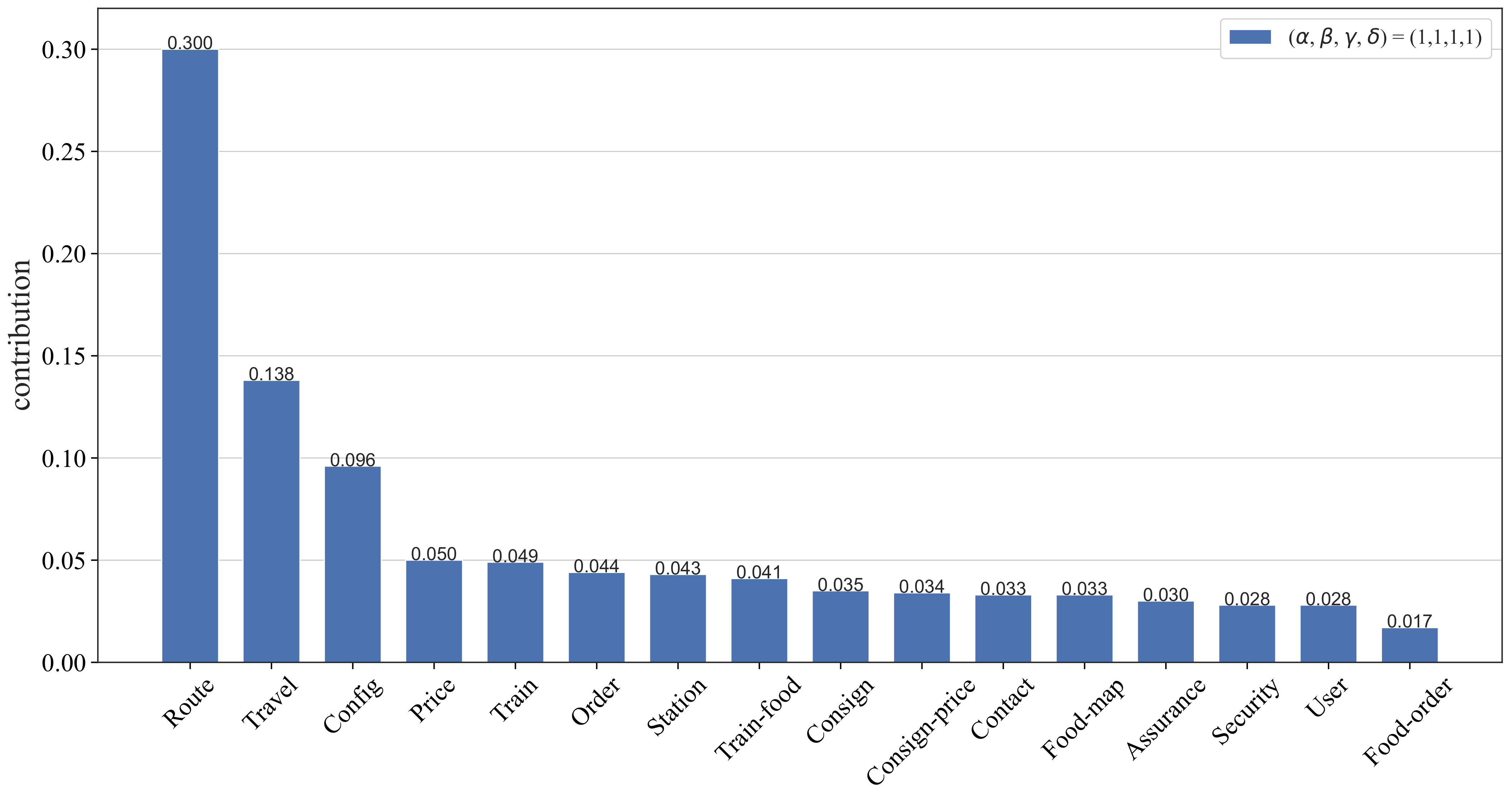
For TrainTicket, when considering business scenarios’ weight (Table 11), the database contributions are shown in Figure 9 (assuming that the four basic operations have the same importance, i.e., α = β = γ = δ = 1 ). Although Travel ranks ninth based on the number of records being operated on, the business scenarios (Advanced search, Travel management) that call Travel are of high importance and therefore make the Travel highly contributive. Order ranks first according to the number of operated records, which is called in the Ticket reservation, and User/Admin order management. However, due to the low importance of the Ticket collect & Enter station in which only Order is called, the contribution of Order is reduced. Contact and User rank fourth and eighth according to the number of operated records, respectively, but the lower contribution of Contact and User is mainly due to the lower importance of Contact management and User management.

4.6. The Impact of Four Basic Operations’ Weight

In this section, we analyze the impact of basic operations’ weight on database contribution based on DBCAMS. As mentioned above, α , β , γ , and δ represent the important weight of the creating, retrieving, updating, and deleting operations, respectively. According to the defined operators in Table 4, the larger the value, the more important the corresponding operation is, and the greater the impact on the database contribution.
We compare the database contributions with the same importance of four operations (i.e., α = β = γ = δ = 1 ) and the database contributions when weighted according to the number of records processed by each operation. Next, we analyze the experimental results of the two systems in detail.

4.6.1. Sock-Shop

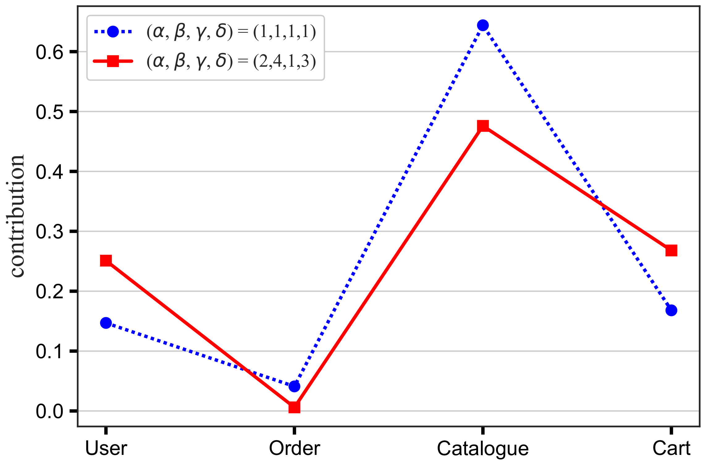
For Sock-Shop, based on Table 5 and Table 9, we obtain the importance weights for four basic operations (i.e., 2, 4, 1, 3). As shown in Figure 10, when the weight is set to ( 2 , 4 , 1 , 3 ) , the ranking of database contributions remains unchanged, but the User and Cart contributions increase slightly, while the Order and Catalogue contributions decrease somewhat. The weight vector ( 2 , 4 , 1 , 3 ) mainly increases the impact of retrieving and deleting operations on the database contribution, i.e., for a specific database, the more records that are queried and deleted, the easier it is to improve the contribution. Specifically, Car management and User information management mainly perform query operations on User, and Purchasing socks and Cart management mainly perform query and deleting operations on Cart, which results in the increased contribution of these two databases. In addition, since both Catalogue and Cart are called by Purchasing socks, the Catalogue contribution decreases. Similarly, User, Order, and Cart are all called by Cart Management, and the contribution of User and Cart increases, so the contribution of Order decreases.

4.6.2. TrainTicket

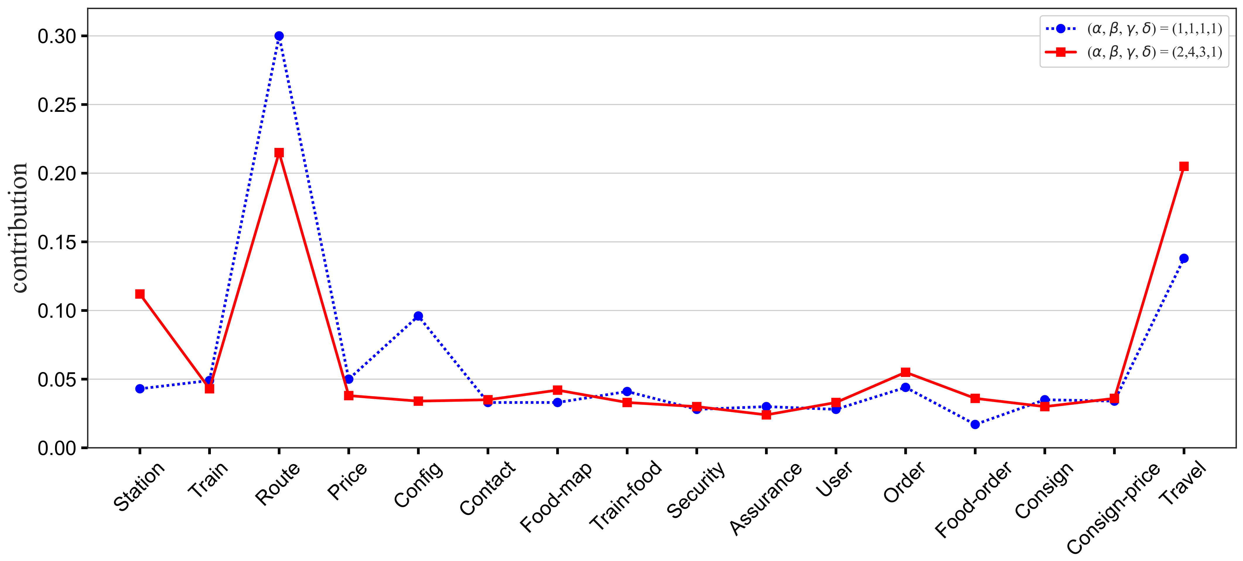
Similarly, for TrainTicket, based on Table 5 and Table 12, we obtain the importance weights for four basic operations (i.e., 2, 4, 3, 1). Figure 11 demonstrates the comparison of the four basic operations weight vector set to ( 1 , 1 , 1 , 1 ) and ( 2 , 4 , 3 , 1 ) . When the weight of the four basic operations is ( 2 , 4 , 3 , 1 ) , which mainly increases the impact of retrieving and updating operations on the database contribution, the overall ranking of the database contribution is basically unchanged, but note that the contributions of Station and Travel increase significantly, the contributions of Route and Config decrease significantly, and the contributions of other databases fluctuate in a small range. Ticket reserve, User order management, and Advanced search all have a large number of retrieving operations on Station, while the retrieving operation has the highest weight, so the contribution of Station has increased notably. The increase in the contribution of Travel is mainly because the number of records retrieved and updated accounts for a high proportion of the number of records processed by all operations. At the same time, Advanced search only calls Station, Train, Route, Price, Config, and Travel, so the contribution of Train, Route, Price, and Config decreases. Because the original contribution of Route and Config is higher, the contribution decreases more.

5. Discussion

In our experiment, we deployed two microservice systems on a single machine with only one instance per database (service). In industrial microservice systems, a service can have several to thousands of instances running on different containers and can be dynamically created or destroyed according to the scaling requirements at runtime [7,12], but this does not affect the effectiveness of our method because these databases (services) can achieve data consistency through related mechanisms [53], which has nothing to do with the database contributions.
By comparing the experimental processes and results of the two systems, we can see that the more business scenarios there are, the lower the efficiency of the AHP process (it is strenuous to construct pairwise comparison matrices). At the same time, the increase of databases in the system may reduce the differentiation between database contributions. An industrial microservice system is usually a large-scale distributed system containing more business scenarios and databases. In this case, more appropriate weighting methods (e.g., G1 method [54], combined weight method [55]) can be considered and try to classify databases and calculate contributions by category.
Since this method aggregates the number of records operated in the business scenario through trace information, the code logic will affect the contribution of the databases. For example, making a large number of redundant calls to a database while implementing a business function may increase the contribution of the database to a certain extent, and because our approach is oriented to business scenarios, different partitions of business scenarios also impact the database contribution.

6. Conclusions

In this study, we proposed a database contribution assessment approach via distributed tracing for microservice systems. This method considers the importance weight of business scenarios, the number of operated records of the database, and the weight of the four basic database operations, so as to skillfully convert the database contribution evaluation into a nonlinear programming problem. The experimental results on two open-source microservice systems demonstrate the validity and rationality of our approach. Future work will focus on the improvement of the optimization efficiency of genetic algorithms in this task and better runtime deployment optimization combined with database contribution.

Author Contributions

Conceptualization, Y.L., Z.Y. and W.K.; methodology, Y.L. and Z.Y.; software, X.Y. and T.D.; validation, X.Y. and W.K.; investigation, Z.F. and C.H.; resources, Z.Y. and C.H.; data curation, Y.L.; writing—original draft preparation, Y.L. and Z.Y.; writing—review and editing, Z.F., C.H. and T.D.; visualization, Z.F.; supervision, C.H.; project administration, T.D. All authors have read and agreed to the published version of the manuscript.

Funding

This research received no external funding.

Institutional Review Board Statement

Not applicable.

Informed Consent Statement

Not applicable.

Data Availability Statement

Not applicable.

Conflicts of Interest

The authors declare no conflict of interest.

Appendix A. Supplementary Details for Experiment on Sock-Shop

Table A1, Table A2, Table A3, Table A4 and Table A5 are the five pairwise comparison matrices scored by experts. Table A6 shows the hierarchical sorting and consistency test of the five pairwise comparison matrices. Table A7 presents the importance weight g of business scenarios represented by the database contribution x of the DBCAMS method.
Table A1. The pairwise comparison matrix C 1 .
BS 1 BS 2 BS 3 BS 4
BS 1 1234
BS 2 1/2123
BS 3 1/31/212
BS 4 1/41/31/21
Table A2. The pairwise comparison matrix C 2 .
BS 1 BS 2 BS 3 BS 4
BS 1 1248
BS 2 1/2137
BS 3 1/41/315
BS 4 1/81/71/51
Table A3. The pairwise comparison matrix C 3 .
BS 1 BS 2 BS 3 BS 4
BS 1 1375
BS 2 1/3153
BS 3 1/71/511/3
BS 4 1/51/331
Table A4. The pairwise comparison matrix C 4 .
BS 1 BS 2 BS 3 BS 4
BS 1 1336
BS 2 1/3113
BS 3 1/3113
BS 4 1/61/31/31
Table A5. The pairwise comparison matrix C 5 .
BS 1 BS 2 BS 3 BS 4
BS 1 1537
BS 2 1/511/33
BS 3 1/3315
BS 4 1/71/31/51
Table A6. The normalized eigenvector and CR of five pairwise comparison matrices. The CR of each matrix is in bold.
BS 1 BS 2 BS 3 BS 4 CR
C 1 0.46730.27720.16010.09540.0115
C 2 0.49770.31540.14340.04360.0445
C 3 0.56500.26220.05530.11750.0433
C 4 0.53460.19630.19630.07280.0076
C 5 0.56500.11750.26220.05530.0433
Table A7. Business scenarios’ importance weights represented by the database contribution x of the DBCAMS method.
Business ScenarioImportance Weight Expression
B S 1 g 1 = 1 5 6 β x 3 + 1 1 6 β x 4
B S 2 g 2 = 1 4 25 β x 1 + 1 5 25 α x 2 + 1 5 25 β + 3 25 γ + 8 25 δ x 4
B S 3 g 3 = 1 2 4 β + 2 4 γ x 1
B S 4 g 4 = 1 β x 2

Appendix B. Supplementary Details for Experiment on TrainTicket

Table A8, Table A9, Table A10, Table A11 and Table A12 are the five pairwise comparison matrices scored by experts for user business scenarios, and Table A13, Table A14, Table A15, Table A16 and Table A17 are the five pairwise comparison matrices scored by experts for administrator business scenarios. Table A18, Table A19 and Table A20 shows the hierarchical sorting and consistency test of the ten pairwise comparison matrices. Table A21 presents the importance weights g of business scenarios represented by the database contribution x of the DBCAMS method.
Table A8. The pairwise comparison matrix User _ C 1 .
BS 1 BS 2 BS 3 BS 4 BS 5
BS 1 1231/25
BS 2 1/2121/43
BS 3 1/31/211/52
BS 4 24517
BS 5 1/51/31/21/71
Table A9. The pairwise comparison matrix User _ C 2 .
BS 1 BS 2 BS 3 BS 4 BS 5
BS 1 11759
BS 2 11759
BS 3 1/71/711/33
BS 4 1/51/5315
BS 5 1/91/91/31/51
Table A10. The pairwise comparison matrix User _ C 3 .
BS 1 BS 2 BS 3 BS 4 BS 5
BS 1 13954
BS 2 1/31753
BS 3 1/91/711/31/4
BS 4 1/51/5311/2
BS 5 1/41/3421
Table A11. The pairwise comparison matrix User _ C 4 .
BS 1 BS 2 BS 3 BS 4 BS 5
BS 1 13524
BS 2 1/5131/22
BS 3 1/91/311/41/2
BS 4 1/34513
BS 5 1/71/531/31
Table A12. The pairwise comparison matrix User _ C 5 .
BS 1 BS 2 BS 3 BS 4 BS 5
BS 1 12435
BS 2 1/21324
BS 3 1/41/311/22
BS 4 1/31/2213
BS 5 1/51/41/21/31
Table A13. The pairwise comparison matrix Admin _ C 1 .
BS 6 BS 7 BS 8 BS 9 BS 10 BS 11 BS 12 BS 13 BS 14
BS 6 1    1/3 1/26   7   3   4   5   2   
BS 7 3   1   2   8   9   5   6   7   4   
BS 8 2    1/21   7   8   4   5   6   3   
BS 9  1/6 1/8 1/71   2    1/4 1/3 1/2 1/5
BS 10  1/7 1/9 1/8 1/21    1/5 1/4 1/3 1/6
BS 11  1/3 1/5 1/44   5   1   2   3    1/2
BS 12  1/4 1/6 1/53   4    1/21   2    1/3
BS 13  1/5 1/7 1/62   3    1/3 1/21    1/4
BS 14  1/2 1/4 1/35   6   2   3   4   1   
Table A14. The pairwise comparison matrix Admin _ C 2 .
BS 6 BS 7 BS 8 BS 9 BS 10 BS 11 BS 12 BS 13 BS 14
BS 6 1   5   5   3   9   7   7   7   8   
BS 7  1/51   1    1/37   5   5   5   3   
BS 8  1/51   1    1/37   5   5   5   3   
BS 9  1/33   3   1   8   6   6   6   2   
BS 10  1/9 1/7 1/7 1/81    1/3 1/3 1/3 1/5
BS 11  1/7 1/5 1/5 1/63   1   1   1    1/3
BS 12  1/7 1/5 1/5 1/63   1   1   1    1/3
BS 13  1/7 1/5 1/5 1/63   1   1   1    1/3
BS 14  1/8 1/3 1/3 1/25   3   3   3   1   
Table A15. The pairwise comparison matrix Admin _ C 3 .
BS 6 BS 7 BS 8 BS 9 BS 10 BS 11 BS 12 BS 13 BS 14
BS 6 1   4   2   6   3   7   8   9   5   
BS 7  1/41    1/33    1/24   5   6   2   
BS 8  1/23   1   5   2   6   7   8   4   
BS 9  1/6 1/3 1/51    1/42   3   4    1/2
BS 10  1/32    1/24   1   5   6   7   3   
BS 11  1/7 1/4 1/6 1/2 1/51   2   3    1/3
BS 12  1/8 1/5 1/7 1/3 1/6 1/21   3    1/4
BS 13  1/9 1/6 1/8 1/4 1/7 1/3 1/31    1/5
BS 14  1/5 1/2 1/42    1/33   4   5   1   
Table A16. The pairwise comparison matrix Admin _ C 4 .
BS 6 BS 7 BS 8 BS 9 BS 10 BS 11 BS 12 BS 13 BS 14
BS 6 1   2    1/24   7    1/35   3   6   
BS 7  1/21    1/33   6    1/44   2   5   
BS 8 2   3   1   5   8    1/26   4   7   
BS 9  1/4 1/3 1/51   4    1/62    1/23   
BS 10  1/7 1/6 1/8 1/41    1/9 1/3 1/5 1/2
BS 11 3   4   2   6   9   1   7   5   8   
BS 12  1/5 1/4 1/6 1/23    1/71    1/32   
BS 13  1/3 1/2 1/42   5    1/53   1   4   
BS 14  1/6 1/5 1/7 1/32    1/8 1/2 1/41   
Table A17. The pairwise comparison matrix Admin _ C 5 .
BS 6 BS 7 BS 8 BS 9 BS 10 BS 11 BS 12 BS 13 BS 14
BS 6 1   4   2   3   7   5   8   6   9   
BS 7  1/41    1/3 1/24   2   5   3   6   
BS 8  1/23   1   2   6   4   7   5   8   
BS 9  1/32    1/21   5   3   6   4   7   
BS 10  1/7 1/4 1/6 1/51    1/32    1/23   
BS 11  1/5 1/2 1/4 1/33   1   4   2   5   
BS 12  1/8 1/5 1/7 1/6 1/2 1/41    1/32   
BS 13  1/6 1/3 1/5 1/42    1/23   1   4   
BS 14  1/9 1/6 1/8 1/7 1/3 1/5 1/2 1/41   
Table A18. The hierarchical single sorting results of User _ C i . The CR of each matrix is in bold.
BS 1 BS 2 BS 3 BS 4 BS 5 CICR
User _ C 1 0.25590.14170.08710.46380.05150.01040.0093
User _ C 2 0.39690.39690.05840.11650.03120.05110.0457
User _ C 3 0.48620.27860.03590.07690.12240.04550.0406
User _ C 4 0.41160.14170.05310.30660.08690.00310.0028
User _ C 5 0.41850.26250.09730.15990.06180.01700.0152
Table A19. The hierarchical single sorting results of Admin _ C i . The CR of each matrix is in bold.
BS 6 BS 7 BS 8 BS 9 BS 10 BS 11 BS 12 BS 13 BS 14 CICR
Admin _ C 1 0.15550.31210.22230.02470.01830.07390.05070.03500.10750.05020.0346
Admin _ C 2 0.37210.12380.12380.19860.01710.03170.03170.03170.06950.07820.0539
Admin _ C 3 0.31130.10750.22190.05070.15530.03500.02650.01780.07390.05660.0391
Admin _ C 4 0.15550.10750.22230.05070.01830.31210.03500.07390.02470.05020.0346
Admin _ C 5 0.31210.10750.22230.15550.03500.07390.02470.05070.01830.05020.0346
Table A20. The hierarchical total sorting results of all business scenarios. The CR_total of each hierarchical total sorting is in bold.
BS 1 BS 2 BS 3 BS 4 BS 5 BS 6 BS 7 BS 8 BS 9 BS 10 BS 11 BS 12 BS 13 BS 14 CR_total
w 1 0.12790.07080.04350.23190.02580.07770.15610.11120.01240.00920.03690.02530.01750.05380.0236
w 2 0.19850.19850.02920.05830.01560.18600.06190.06190.09930.00850.01590.01590.01590.03470.0503
w 3 0.24310.13930.01790.03850.06120.15560.05380.11100.02540.07770.01750.01330.00890.03700.0397
w 4 0.20580.07090.02660.15330.04340.07770.05380.11120.02530.00920.15610.01750.03690.01240.0207
w 5 0.20930.13130.04860.08000.03090.15610.05380.11120.07770.01750.03690.01240.02530.00920.0261
Table A21. Business scenarios’ importance weights represented by the database contribution x of the DBCAMS method.
Business ScenarioImportance Weight Expression
B S 1 g 1 = 1 51 129.5 β x 1 + 1 22 129.5 β x 2 + 1 28.5 129.5 β x 3 + 1 6 129.5 β x 4 + 1 10 129.5 β x 5 + 1 1 129.5 β x 6 + 1 3 129.5 β x 7 + 1 0.5 129.5 β x 8 + 1 2 129.5 β x 9 + 1 1 129.5 α x 10 + 1 1 129.5 β x 11 + 1 1 129.5 α x 12 + 1 0.5 129.5 α x 13 + 1 1 129.5 α x 14 + 1 1 129.5 β x 15
B S 2 g 2 = 1 300 784 β x 1 + 1 130 784 β x 2 + 1 160 784 β x 3 + 1 30 784 β x 4 + 1 60 784 β x 5 + 1 10 784 β x 11 + 1 60 784 β + 30 784 γ x 12 + 1 2 784 β x 14 + 1 2 784 β x 15
B S 3 g 3 = 1 β x 14
B S 4 g 4 = 1 58 138 β x 1 + 1 24 138 β x 2 + 1 35 138 β x 3 + 1 4 138 β x 4 + 1 16 138 β x 5 + 1 1 138 β x 16
B S 5 g 5 = 1 2 4 β + 2 4 γ x 12
B S 6 g 6 = 1 200 1000 α + 400 1000 β + 200 1000 γ + 200 1000 δ x 12
B S 7 g 7 = 1 5 25 α + 10 25 β + 5 25 γ + 5 25 δ x 3
B S 8 g 8 = 1 10 35 β x 2 + 1 10 35 β x 3 + 1 5 35 α + 5 35 γ + 5 35 δ x 16
B S 9 g 9 = 1 10 50 α + 20 50 β + 10 50 γ + 10 50 δ x 11
B S 10 g 10 = 1 40 200 α + 80 200 β + 40 200 γ + 40 200 δ x 6
B S 11 g 11 = 1 7 34 α + 13 34 β + 7 34 γ + 7 34 δ x 1
B S 12 g 12 = 1 3 15 α + 6 15 β + 3 15 γ + 3 15 δ x 2
B S 13 g 13 = 1 5 25 α + 10 25 β + 5 25 γ + 5 25 δ x 4
B S 14 g 14 = 1 1 4 α + 1 4 β + 1 4 γ + 1 4 δ x 5

References

  1. Lewis, J.; Fowler, M. Microservices a Definition of This New Architectural Term. 2014. Available online: http://martinfowler.com/articles/microservices.html (accessed on 24 October 2022).
  2. Richardson, C. Microservices Patterns: With Examples in Java; Manning: New York, NY, USA, 2018. [Google Scholar]
  3. Guo, X.; Peng, X.; Wang, H.; Li, W.; Jiang, H.; Ding, D.; Xie, T.; Su, L. Graph-Based Trace Analysis for Microservice Architecture Understanding and Problem Diagnosis. In ESEC/FSE 2020: Proceedings of the 28th ACM Joint Meeting on European Software Engineering Conference and Symposium on the Foundations of Software Engineering; Association for Computing Machinery: New York, NY, USA, 2020; pp. 1387–1397. [Google Scholar] [CrossRef]
  4. Zhou, X.; Peng, X.; Xie, T.; Sun, J.; Ji, C.; Li, W.; Ding, D. Fault Analysis and Debugging of Microservice Systems: Industrial Survey, Benchmark System, and Empirical Study. IEEE Trans. Softw. Eng. 2021, 47, 243–260. [Google Scholar] [CrossRef] [Green Version]
  5. Francesco, P.D.; Malavolta, I.; Lago, P. Research on Architecting Microservices: Trends, Focus, and Potential for Industrial Adoption. In Proceedings of the 2017 IEEE International Conference on Software Architecture (ICSA), Gothenburg, Sweden, 3–7 April 2017; pp. 21–30. [Google Scholar] [CrossRef] [Green Version]
  6. Xiang, Q.; Peng, X.; He, C.; Wang, H.; Xie, T.; Liu, D.; Zhang, G.; Cai, Y. No Free Lunch: Microservice Practices Reconsidered in Industry. arXiv 2021, arXiv:2106.07321. [Google Scholar] [CrossRef]
  7. Liu, D.; He, C.; Peng, X.; Lin, F.; Zhang, C.; Gong, S.; Li, Z.; Ou, J.; Wu, Z. MicroHECL: High-Efficient Root Cause Localization in Large-Scale Microservice Systems. In Proceedings of the 2021 IEEE/ACM 43rd International Conference on Software Engineering: Software Engineering in Practice (ICSE-SEIP), Madrid, Spain, 25–28 May 2021; pp. 338–347. [Google Scholar] [CrossRef]
  8. Ding, D.; Peng, X.; Guo, X.; Zhang, J.; Wu, Y. Scenario-driven and bottom-up microservice decomposition for monolithic systems. J. Softw. 2020, 31, 3461–3480. [Google Scholar] [CrossRef]
  9. Zhang, C.; Peng, X.; Sha, C.; Zhang, K.; Fu, Z.; Wu, X.; Lin, Q.; Zhang, D. DeepTraLog: Trace-Log Combined Microservice Anomaly Detection through Graph-based Deep Learning. In Proceedings of the 44th International Conference on Software Engineering, Pittsburgh, PA, USA, 25–27 May 2022; pp. 623–634. [Google Scholar] [CrossRef]
  10. Sampaio, A.R.; Rubin, J.; Beschastnikh, I.; Rosa, N.S. Improving microservice-based applications with runtime placement adaptation. J. Internet Serv. Appl. 2019, 10, 4. [Google Scholar] [CrossRef]
  11. Ma, W.; Wang, R.; Gu, Y.; Meng, Q.; Huang, H.; Deng, S.; Wu, Y. Multi-objective microservice deployment optimization via a knowledge-driven evolutionary algorithm. Complex Intell. Syst. 2021, 7, 1153–1171. [Google Scholar] [CrossRef]
  12. Li, B.; Peng, X.; Xiang, Q.; Wang, H.; Xie, T.; Sun, J.; Liu, X. Enjoy your observability: An industrial survey of microservice tracing and analysis. Empir. Softw. Eng. 2022, 27, 25. [Google Scholar] [CrossRef] [PubMed]
  13. Wang, K.; Li, K.; Gao, J.; Liu, B.; Fang, Z.; Ke, W. A Quantitative Evaluation Method of Software Usability Based on Improved GOMS Model. In Proceedings of the 2021 IEEE 21st International Conference on Software Quality, Reliability and Security Companion (QRS-C), Hainan, China, 6–10 December 2021; pp. 691–697. [Google Scholar] [CrossRef]
  14. Saaty, T.L. How to make a decision: The analytic hierarchy process. Eur. J. Oper. Res. 1990, 48, 9–26. [Google Scholar] [CrossRef]
  15. Sockshop. Available online: https://github.com/microservices-demo/microservices-demo (accessed on 3 September 2022).
  16. TrainTicket. Available online: https://github.com/FudanSELab/train-ticket/releases/tag/v0.2.0 (accessed on 3 September 2022).
  17. Sridharan, C. Distributed Systems Observability: A Guide to Building Robust Systems; O’Reilly Media: Sebastopol, CA, USA, 2018. [Google Scholar]
  18. Sigelman, B.H.; Barroso, L.A.; Burrows, M.; Stephenson, P.; Plakal, M.; Beaver, D.; Jaspan, S.; Shanbhag, C. Dapper, a Large-Scale Distributed Systems Tracing Infrastructure; Technical Report; Google, Inc.: Mountain View, CA, USA, 2010. [Google Scholar]
  19. Pinpoint. Available online: https://github.com/pinpoint-apm/pinpoint (accessed on 4 September 2022).
  20. OpenZipkin. Available online: https://zipkin.io/ (accessed on 4 September 2022).
  21. Jaeger. Available online: https://www.jaegertracing.io/ (accessed on 4 September 2022).
  22. Apache Skywalking. Available online: https://skywalking.apache.org/ (accessed on 4 September 2022).
  23. The OpenTracing Project. Available online: https://opentracing.io/ (accessed on 4 September 2022).
  24. OpenCensus. Available online: https://opencensus.io/ (accessed on 4 September 2022).
  25. OpenTelemetry. Available online: https://opentelemetry.io/ (accessed on 4 September 2022).
  26. Zhou, X.; Peng, X.; Xie, T.; Sun, J.; Ji, C.; Liu, D.; Xiang, Q.; He, C. Latent Error Prediction and Fault Localization for Microservice Applications by Learning from System Trace Logs. In ESEC/FSE 2019: Proceedings of the 2019 27th ACM Joint Meeting on European Software Engineering Conference and Symposium on the Foundations of Software Engineering; Association for Computing Machinery: New York, NY, USA, 2019; pp. 683–694. [Google Scholar] [CrossRef]
  27. Liu, P.; Xu, H.; Ouyang, Q.; Jiao, R.; Chen, Z.; Zhang, S.; Yang, J.; Mo, L.; Zeng, J.; Xue, W.; et al. Unsupervised Detection of Microservice Trace Anomalies through Service-Level Deep Bayesian Networks. In Proceedings of the 2020 IEEE 31st International Symposium on Software Reliability Engineering (ISSRE), Coimbra, Portugal, 12–15 October 2020; pp. 48–58. [Google Scholar] [CrossRef]
  28. Bogner, J.; Schlinger, S.; Wagner, S.; Zimmermann, A. A Modular Approach to Calculate Service-Based Maintainability Metrics from Runtime Data of Microservices. In Product-Focused Software Process Improvement. PROFES 2019; Franch, X., Männistö, T., Martínez-Fernández, S., Eds.; Lecture Notes in Computer Science; Springer: Cham, Switzerland, 2019; pp. 489–496. [Google Scholar]
  29. Bonacich, P. Factoring and weighting approaches to status scores and clique identification. J. Math. Sociol. 1972, 2, 113–120. [Google Scholar] [CrossRef]
  30. Chen, D.; Lü, L.; Shang, M.S.; Zhang, Y.C.; Zhou, T. Identifying influential nodes in complex networks. Phys. A Stat. Mech. Its Appl. 2012, 391, 1777–1787. [Google Scholar] [CrossRef] [Green Version]
  31. Kitsak, M.; Gallos, L.K.; Havlin, S.; Liljeros, F.; Muchnik, L.; Stanley, H.E.; Makse, H.A. Identification of influential spreaders in complex networks. Nat. Phys. 2010, 6, 888–893. [Google Scholar] [CrossRef] [Green Version]
  32. Hage, P.; Harary, F. Eccentricity and centrality in networks. Soc. Netw. 1995, 17, 57–63. [Google Scholar] [CrossRef]
  33. Stephenson, K.; Zelen, M. Rethinking centrality: Methods and examples. Soc. Netw. 1989, 11, 1–37. [Google Scholar] [CrossRef]
  34. Estrada, E.; Rodríguez-Velázquez, J.A. Subgraph centrality in complex networks. Phys. Rev. E 2005, 71, 056103. [Google Scholar] [CrossRef] [PubMed]
  35. Poulin, R.; Boily, M.C.; Mâsse, B. Dynamical systems to define centrality in social networks. Soc. Netw. 2000, 22, 187–220. [Google Scholar] [CrossRef]
  36. Brin, S.; Page, L. The anatomy of a large-scale hypertextual Web search engine. Comput. Netw. ISDN Syst. 1998, 30, 107–117. [Google Scholar] [CrossRef]
  37. Lü, L.; Zhang, Y.C.; Yeung, C.H.; Zhou, T. Leaders in social networks, the delicious case. PLoS ONE 2011, 6, e21202. [Google Scholar] [CrossRef] [Green Version]
  38. Kleinberg, J.M. Authoritative Sources in a Hyperlinked Environment. J. ACM 1999, 46, 604–632. [Google Scholar] [CrossRef] [Green Version]
  39. Lempel, R.; Moran, S. The stochastic approach for link-structure analysis (SALSA) and the TKC effect1Abridged version1. Comput. Netw. 2000, 33, 387–401. [Google Scholar] [CrossRef] [Green Version]
  40. Dangalchev, C. Residual closeness in networks. Phys. A Stat. Mech. Its Appl. 2006, 365, 556–564. [Google Scholar] [CrossRef]
  41. Lü, L.; Chen, D.; Ren, X.L.; Zhang, Q.M.; Zhang, Y.C.; Zhou, T. Vital nodes identification in complex networks. Phys. Rep. 2016, 650, 1–63. [Google Scholar] [CrossRef] [Green Version]
  42. Gousios, G.; Kalliamvakou, E.; Spinellis, D. Measuring Developer Contribution from Software Repository Data. In MSR ’08: Proceedings of the 2008 International Working Conference on Mining Software Repositories; Association for Computing Machinery: New York, NY, USA, 2008; pp. 129–132. [Google Scholar] [CrossRef] [Green Version]
  43. Zhou, M.; Mockus, A. Who Will Stay in the FLOSS Community? Modeling Participant’s Initial Behavior. IEEE Trans. Softw. Eng. 2015, 41, 82–99. [Google Scholar] [CrossRef]
  44. Wang, G.; Dang, C.X.; Zhou, Z. Measure Contribution of Participants in Federated Learning. In Proceedings of the 2019 IEEE International Conference on Big Data (Big Data), Los Angeles, CA, USA, 9–12 December 2019; pp. 2597–2604. [Google Scholar] [CrossRef]
  45. Boyer, S.; Ikeda, T.; Lefort, M.C.; Malumbres-Olarte, J.; Schmidt, J.M. Percentage-based Author Contribution Index: A universal measure of author contribution to scientific articles. Res. Integr. Peer Rev. 2017, 2, 18. [Google Scholar] [CrossRef] [Green Version]
  46. Al-Harbi, K.M.S. Application of the AHP in project management. Int. J. Proj. Manag. 2001, 19, 19–27. [Google Scholar] [CrossRef]
  47. Vaidya, O.S.; Kumar, S. Analytic hierarchy process: An overview of applications. Eur. J. Oper. Res. 2006, 169, 1–29. [Google Scholar] [CrossRef]
  48. Saaty, T.L. A scaling method for priorities in hierarchical structures. J. Math. Psychol. 1977, 15, 234–281. [Google Scholar] [CrossRef]
  49. Harada, T.; Alba, E. Parallel Genetic Algorithms: A Useful Survey. ACM Comput. Surv. 2020, 53, 86. [Google Scholar] [CrossRef]
  50. Quint, P.; Kratzke, N. Towards a Lightweight Multi-Cloud DSL for Elastic and Transferable Cloud-native Applications. In Proceedings of the 8th International Conference on Cloud Computing and Services Science, CLOSER 2018, Funchal, Portugal, 19–21 March 2018; pp. 400–408. [Google Scholar] [CrossRef]
  51. Brogi, A.; Rinaldi, L.; Soldani, J. TosKer: A synergy between TOSCA and Docker for orchestrating multicomponent applications. Softw. Pract. Exp. 2018, 48, 2061–2079. [Google Scholar] [CrossRef]
  52. Gretton, A.; Borgwardt, K.; Rasch, M.; Schölkopf, B.; Smola, A. A Kernel Method for the Two-Sample-Problem. In Advances in Neural Information Processing Systems 19 (NIPS 2006); Schölkopf, B., Platt, J., Hoffman, T., Eds.; MIT Press: Cambridge, CA, USA, 2006; Volume 19. [Google Scholar]
  53. Viennot, N.; Lécuyer, M.; Bell, J.; Geambasu, R.; Nieh, J. Synapse: A Microservices Architecture for Heterogeneous-Database Web Applications. In EuroSys ’15: Proceedings of the Tenth European Conference on Computer Systems; Association for Computing Machinery: New York, NY, USA, 2015; pp. 1–16. [Google Scholar] [CrossRef]
  54. Gu, Y.; Xie, J.; Liu, H.; Yang, Y.; Tan, Y.; Chen, L. Evaluation and analysis of comprehensive performance of a brake pedal based on an improved analytic hierarchy process. Proc. Inst. Mech. Eng. Part D J. Automob. Eng. 2021, 235, 2636–2648. [Google Scholar] [CrossRef]
  55. Wang, Q.; Zhao, D.; Yang, B.; Li, C. Risk assessment of the UPIoT construction in China using combined dynamic weighting method under IFGDM environment. Sustain. Cities Soc. 2020, 60, 102199. [Google Scholar] [CrossRef]
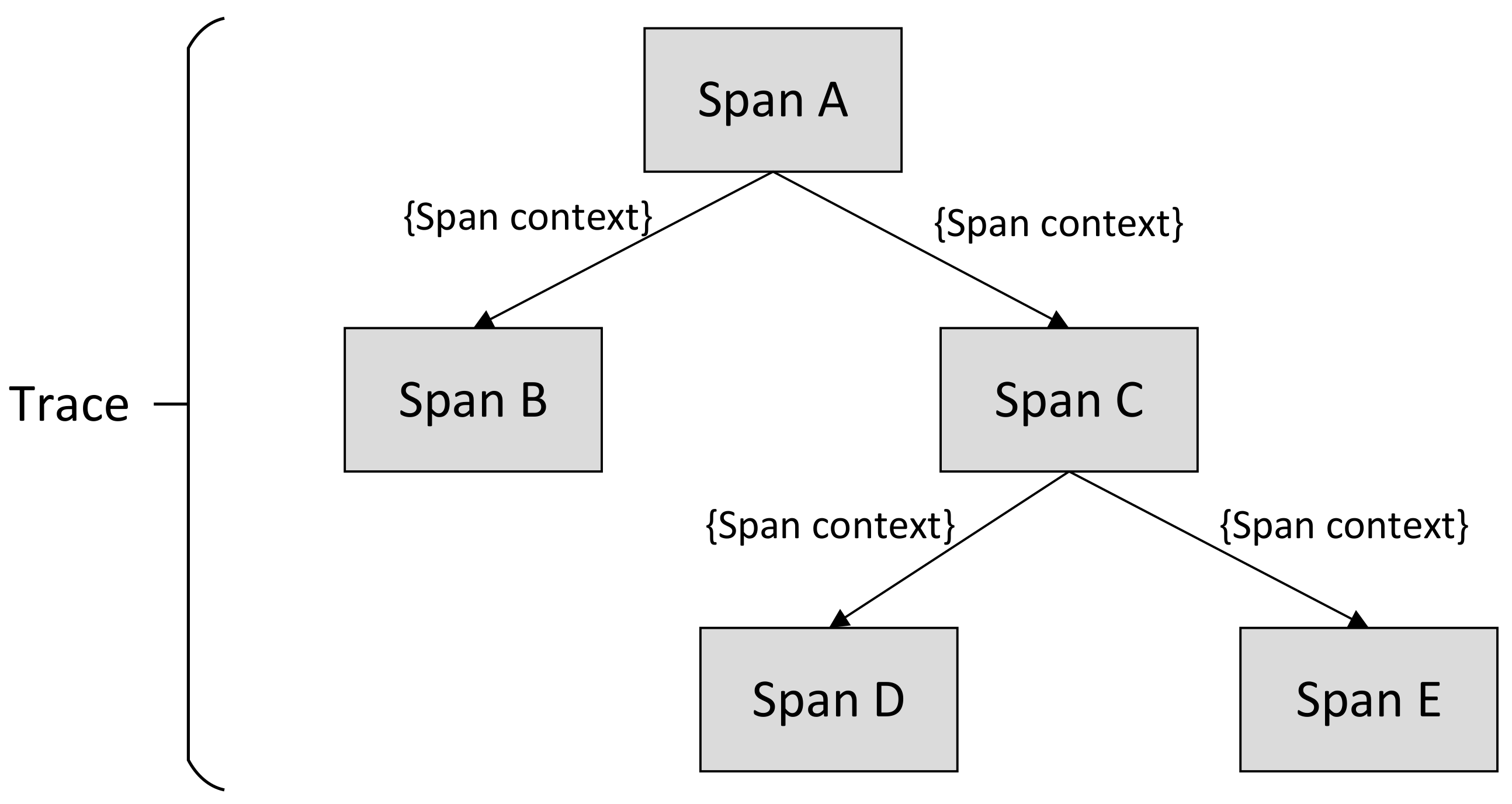
Figure 1. Traces and spans in distributed tracing.
Applsci 12 11488 g001
Figure 2. An example of a general microservice system. The main practical influence of the calculated database contribution is to provide information for runtime deployment optimization.
Applsci 12 11488 g002
Figure 3. Framework of our method.
Applsci 12 11488 g003
Figure 4. Business scenarios hierarchy model.
Applsci 12 11488 g004
Figure 5. A typical process of Purchasing socks in Sock-Shop.
Applsci 12 11488 g005
Figure 6. The business scenarios hierarchy of Sock-Shop. We denote the four business scenarios of Purchasing socks, Cart management, User information management, and Historical orders query as B S 1 , B S 2 , B S 3 , and B S 4 , respectively.
Applsci 12 11488 g006
Figure 7. The business scenarios hierarchy of TrainTicket. The fourteen business scenarios are divided into two categories: user and administrator. We denote the fourteen business scenarios of Ticket reserve, User order management, …, and Config management as B S 1 , B S 2 , …, and B S 14 , respectively.
Applsci 12 11488 g007
Figure 8. The database contributions to business scenarios in Sock-Shop.
Applsci 12 11488 g008
Figure 9. The database contributions to business scenarios in TrainTicket.
Applsci 12 11488 g009
Figure 10. The database contributions to business scenarios in Sock-Shop.
Applsci 12 11488 g010
Figure 11. The database contributions to business scenarios in TrainTicket.
Applsci 12 11488 g011
Table 1. Pairwise comparison scale for AHP.
Intensity of ImportanceDescripition
1Equal importance
3Moderate importance of one over another
5Essential or strong importance
7Very strong importance
9Extreme importance
2, 4, 6, 8Intermediate values between the two adjacent judgments
ReciprocalsValues for inverse comparison
Table 2. Average random consistency (RI).
Order of Matrix345678910
RI0.580.901.121.241.321.411.451.49
Table 3. Span tags in a span of Catalogue service. The span ID is 7b5af686fc795d70 and span name is GET/catalogue/{id}.
KeyValue
http.methodGET
http.urlcatalogue/03fef6ac-18964ce8-bd69-b798f85c6e0b
internal.span.formatzipkin
span.kindserver
Table 4. The definitions of operators for the four basic database operations 1 k n , 1 i m .
OperationOperator
Create h records on the k-th database in the i-th business scenario. 1 h N i · α x k   
Retrieve h records on the k-th database in the i-th business scenario. 1 h N i · β x k   
Update h records on the k-th database in the i-th business scenario. 1 h N i · γ x k   
Delete h records on the k-th database in the i-th business scenario. 1 h N i · δ x k
Table 5. The equations of counting records operated by four basic operations.
OperationEquation
Create i = 1 m k = 1 n c i k   
Retrieve i = 1 m k = 1 n r i k   
Update i = 1 m k = 1 n u i k   
Delete i = 1 m k = 1 n d i k
Table 6. Descriptions and settings of databases in Sock-Shop.
DatabaseIdentifierDescriptionNumber of Records
User D B 1 Including user name, shipping address, bank card, etc.3
Order D B 2 Including orderID, date, total amount, order status, etc.10 per user
Catalogue D B 3 Including itemID, item name, image URL, price, details, quantity, tag, etc.9
Cart D B 4 Including item name, quantity, unit price, discount, total price, etc.5 per user
Table 7. Descriptions and settings of databases in TrainTicket.
DatabaseIdentifierDescriptionNumber of Records
Station D B 1 Including stationID, stationName, stayTime, etc.13
Train D B 2 Including trainTypeID, averageSpeed, etc.6
Route D B 3 Including routeID, passingStations, distances, startStationId, etc.10
Price D B 4 Including priceRatioID, routeId, trainType, basicPriceRate, etc.10
Config D B 5 Including configName, value, description, etc.1
Contact D B 6 Including contactID, userId, name, phoneNumber, etc.4 per user
Food-map D B 7 Including foodStoreID, stationID, foodlist, etc.6
Train-food D B 8 Including ID, travelID, foodlist, etc.5
Security D B 9 Including securityConfigID, name, description, etc.1
Assurance D B 10 Including assuranceID, orderID, assuranceType, etc.10 per user
User D B 11 Including userID, userName, password, gender, email, etc.20
Order D B 12 Including orderID, bought date, userID, passenger, status, price, etc.20 per user
Food-order D B 13 Including foodOrderID, foodType, foodName, price, etc.10 per user
Consign D B 14 Including consignID, consignee, price, phone, weight, etc.4 per user
Consign-price D B 15 Including consign-priceID, initialWeight, initialPrice, etc.1
Travel D B 16 Including travelID, trainTypeID, routeID, startingStation, terminalStation, etc.10
Table 8. The importance weight of business scenarios in Sock-Shop.
BS 1 BS 2 BS 3 BS 4
w ¯ 0.52590.23370.16350.0769
Table 9. The aggregation results of business scenarios in Sock-Shop.
Business ScenarioAggregation Result N i
Purchasing socks D B 3 : r5 1; D B 4 : c16
Cart management D B 1 : r4; D B 2 : c5; D B 4 : r5, u3, d825
User information management D B 1 : u2, r24
Historical order query D B 2 : r1515
1 D B 3 :r5 denotes retrieving 5 records on the D B 3 , and the rest are similar; c, r, u, and d represent creating, retrieving, updating, and deleting respectively.
Table 10. The main results of Sock-Shop. The best result of L2-Norm is underlined, and the databases’ contributions of the corresponding method are bold. ( α , β , γ , δ = 2 , 4 , 1 , 3 ).
RankingDBCAMSDBCAMS-MMDDBCAMS-RN
DatabaseContributionDatabaseContributionDatabaseContribution
1Catalogue0.476Catalogue0.698Catalogue0.713
2Cart0.268User0.194Cart0.120
3User0.251Cart0.087Order0.089
4Order0.006Order0.022User0.077
L2-Norm0.14560.20650.1829
Table 11. The importance weight of business scenarios in TrainTicket.
BS 1 BS 2 BS 3 BS 4 BS 5 BS 6 BS 7 BS 8 BS 9 BS 10 BS 11 BS 12 BS 13 BS 14
w ¯ 0.19690.12220.03320.11240.03540.13060.07580.10130.04800.02440.05270.01690.02090.0294
Table 12. The aggregation results of business scenarios in TrainTicket.
Business ScenarioAggregation Result N i
B S 1 D B 1 : r51; D B 2 : r22; D B 3 : r28.5; D B 4 : r6; D B 5 : r10; D B 6 : r1; D B 7 : r3; D B 8 : r0.5; D B 9 : r2; D B 10 : c1; D B 11 : r1; D B 12 : c1; D B 13 : c0.5; D B 14 : c1; D B 15 : r1129.5
B S 2 D B 1 : r300; D B 2 : r130; D B 3 : r160; D B 4 : r30; D B 5 : r60; D B 11 : r10; D B 12 : r60, u30; D B 14 : u2; D B 15 : r2784
B S 3 D B 14 : r44
B S 4 D B 1 : r58; D B 2 : r24; D B 3 : r35; D B 4 : r4; D B 5 : r16; D B 16 : r1138
B S 5 D B 12 : r2, u24
B S 6 D B 12 : c200, r400, u200, d2001000
B S 7 D B 3 : c5, r10, u5, d525
B S 8 D B 2 : r10; D B 3 : r10; D B 16 : c5, u5, d535
B S 9 D B 11 : c10, r20, u10, d1050
B S 10 D B 6 : c40, r80, u40, d40200
B S 11 D B 1 : c7, r13, u7, d734
B S 12 D B 2 : c3, r6, u3, d315
B S 13 D B 4 : c5, r10, u5, d525
B S 14 D B 5 : c1, r1, u1, d14
Table 13. The main results of TrainTicket. The best result of L2-Norm is underlined, and the databases’ contributions of the corresponding method are in bold ( α , β , γ , δ = 2 , 4 , 3 , 1 ).
RankingDBCAMSDBCAMS-MMDDBCAMS-RN
DatabaseContributionDatabaseContributionDatabaseContribution
1Route0.215Station0.609Route0.279
2Travel0.205Train0.068Travel0.195
3Station0.112Security0.062Food-map0.053
4Order0.055Food-map0.054User0.050
5Train0.043Config0.042Consign0.046
6Food-map0.042Assurance0.027Order0.045
7Price0.038Order0.026Food-order0.043
8Food-order0.036Contact0.022Config0.042
9Consign-price0.036Price0.019Train-food0.041
10Contact0.035Food-order0.017Price0.041
11Config0.034Consign-price0.015Train0.039
12Train-food0.033Train-food0.012Consign-price0.029
13User0.033User0.011Station0.028
14Security0.030Route0.007Contact0.026
15Consign0.030Travel0.005Assurance0.024
16Assurance0.024Consign0.002Security0.019
L2-Norm0.35580.44580.4276
Table 14. Optimization effects of different algorithms. The best results are in bold, and the second best ones are underlined. The hyperparameters in the heuristic algorithm are set to empirical values that work well.
SystemCategoryAlgorithmL2-Norm
Sock-ShopTraditionalInterior point0.1548
SQP0.1546
HeuristicSA0.1451
PSO0.1432
GA0.1429
TrainTicketTraditionalInterior point0.3902
SQP0.3898
HeuristicSA0.3617
PSO0.3555
GA0.3558
Table 15. s k and contribution ranking of databases in Sock-Shop.
Database s k Contribution Ranking
User83
Order201
Catalogue54
Cart172
Table 16. s k and contribution ranking of databases in TrainTicket.
Database s k Contribution Ranking
Station4432
Train2014
Route258.53
Price657
Config906
Contact2014
Food-map311
Train-food0.515
Security213
Assurance114
User618
Order10951
Food-order0.515
Consign710
Consign-price311
Travel169
Publisher’s Note: MDPI stays neutral with regard to jurisdictional claims in published maps and institutional affiliations.