
A Visual Feedback for Water-Flow Monitoring in Recirculating Aquaculture Systems

 ,
,  ,
,  ,
,  , , and
Abstract
1. Introduction
2. Materials and Methods
2.1. Experimental Site
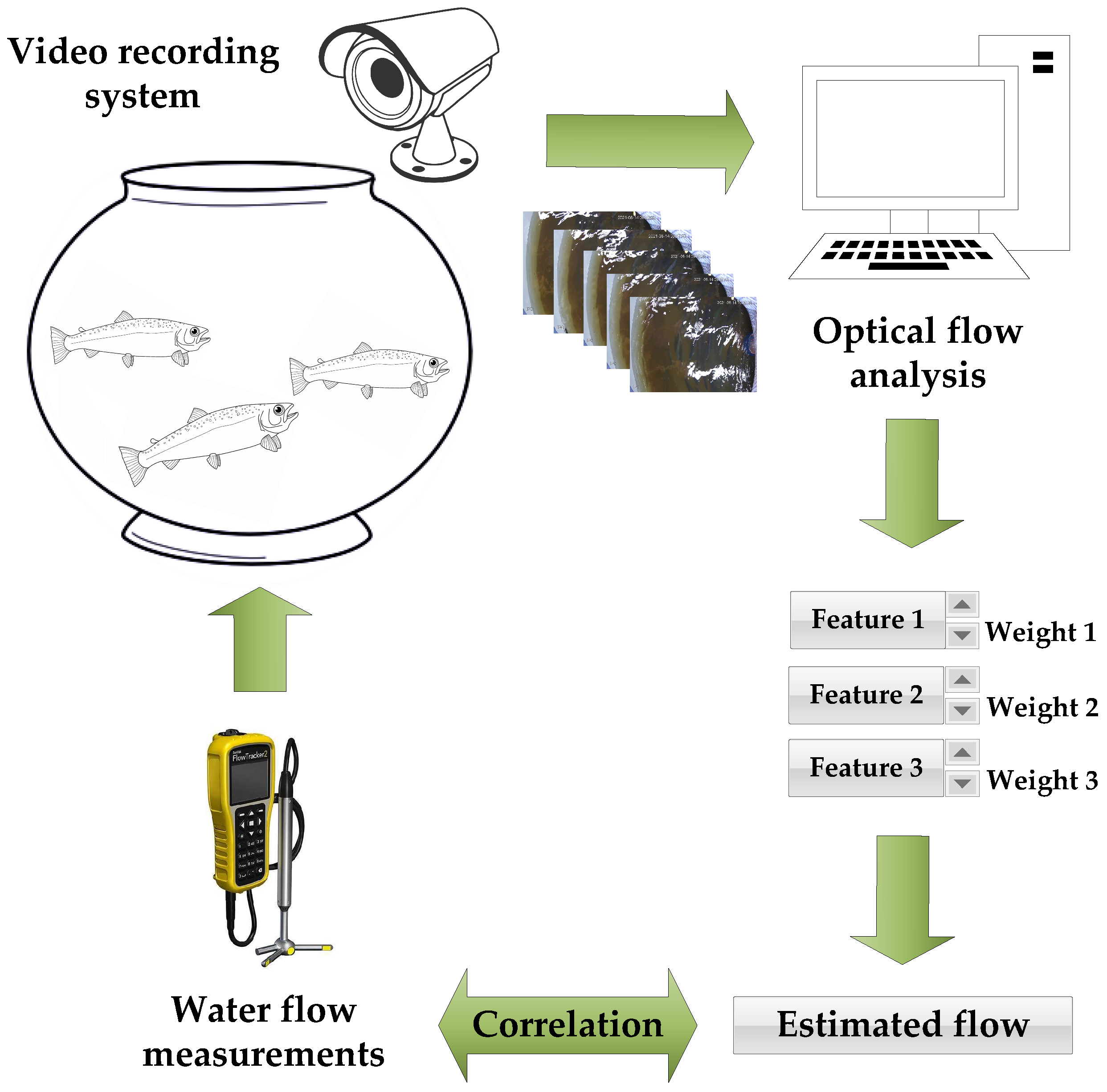
2.2. The Overview of the Applied Optical Flow Methods
- Horn–Schunck (HS) method;
- Farneback (F) method;
- Lucas–Kanade (LK) method.
- Determining the values of the directional gradients and using the convolutional filter with the mask and its transposed version, respectively;
- Calculation of the differential value between the frames;
- Smoothing the gradients and using the pixels convolutional filter with the mask type ;
- Solving the system of two linear equations for each pixel:using the eigenvalues of the matrix A determined as and . Both those values are compared to the threshold applied for the reduction in the noise effect. If at least the threshold value is obtained by both eigenvalues, the system of equations can be solved by Cramer’s method. When both eigenvalues are less than the threshold , the optical flow is zero, whereas if only (and ), the matrix A is singular and the gradient flow is normalized to calculate u and v values. The default threshold value is .
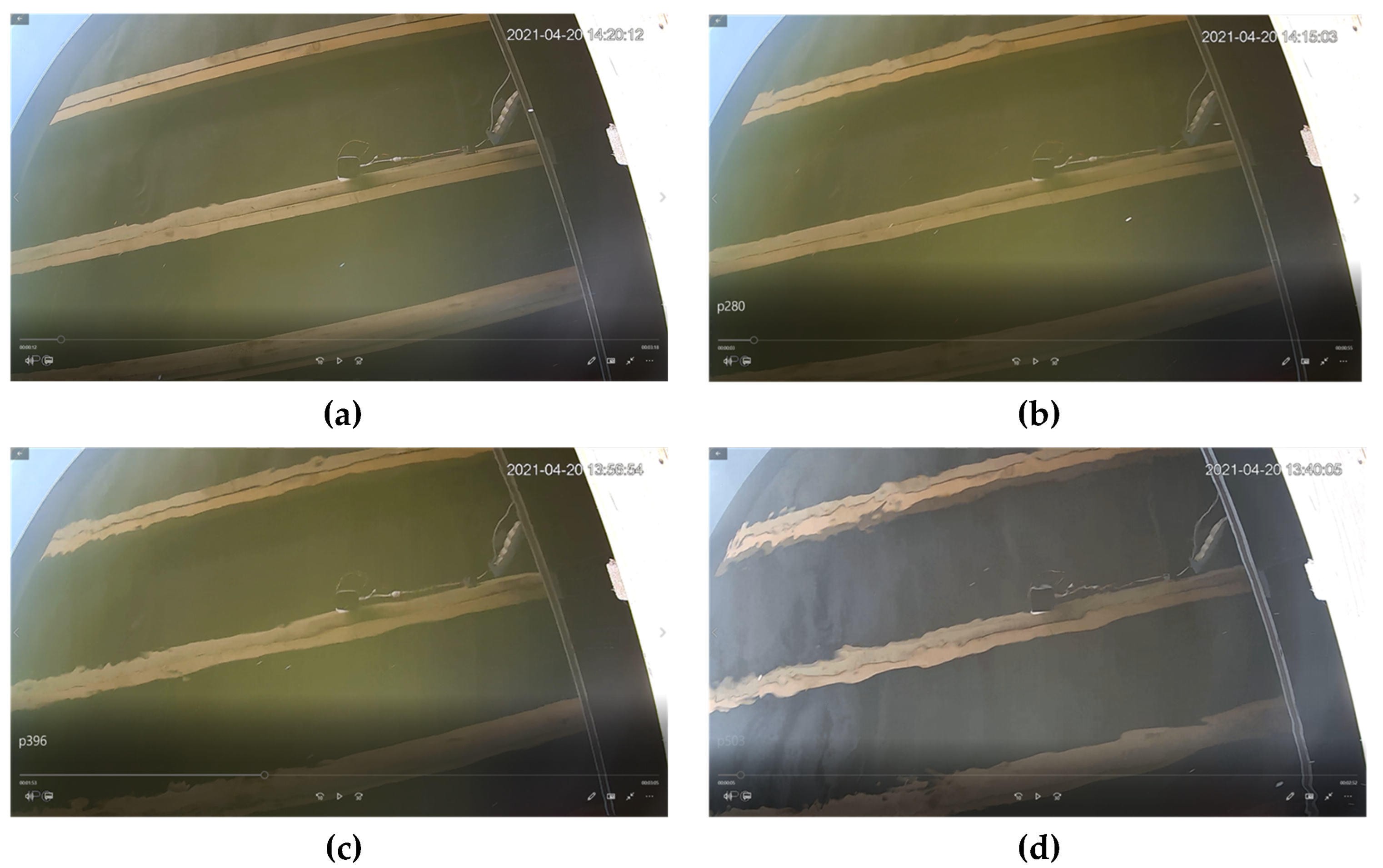
2.3. Experiments
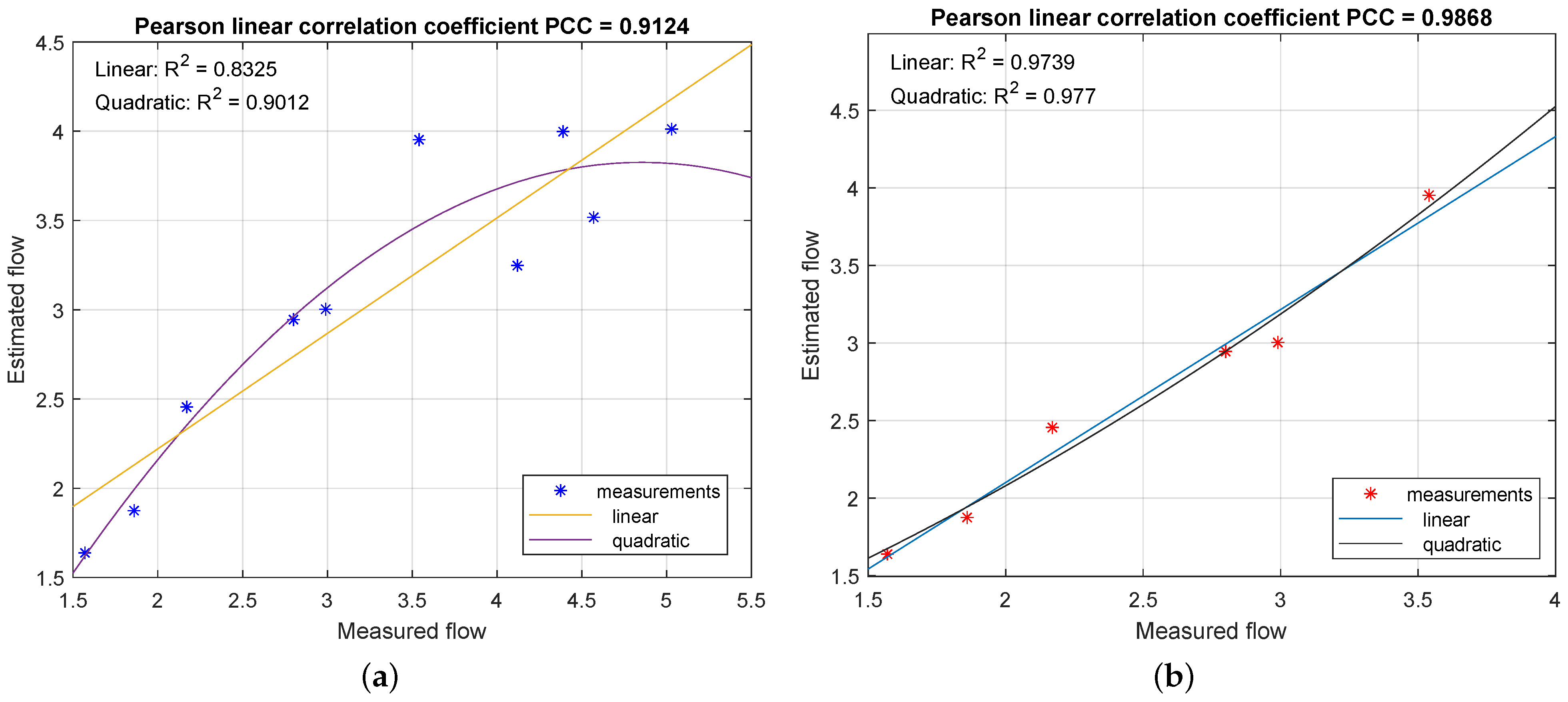
3. Discussion of the Experimental Results
- Squared entropy of the motion vectors map for the Farneback method ();
- Standard deviation of the motion vector map for the Lucas–Kanade method ();
- Variance in the local entropy of the motion vector map for the Lucas–Kanade method ().
4. Conclusions
Author Contributions
Funding
Institutional Review Board Statement
Informed Consent Statement
Data Availability Statement
Conflicts of Interest
Abbreviations
| AFMV | Airborne feature matching velocimetry |
| BLC | Back light compensation |
| CMOS | Complementary metal-oxide-semiconductor |
| CNN | Convolutional neural network |
| DC | direct current |
| FPGA | Field-programmable gate array |
| HLC | High light compensation |
| ICR | Infrared cutfilter removal |
| IoT | Internet of Things |
| IR | Infrared |
| JPEG | Joint Photographic Experts Group |
| LED | Light-emitting diode |
| MJPEG | Motion JPEG |
| PoE | Power over Ethernet |
| PIV | Particle image velocimetry |
| RAS | Recirculating Aquaculture System |
| RoI | Region of interest |
| WDR | Wide dynamic range |
References
- Liu, Y.; Ma, X.; Shu, L.; Hancke, G.P.; Abu-Mahfouz, A.M. From Industry 4.0 to Agriculture 4.0: Current Status, Enabling Technologies, and Research Challenges. IEEE Trans. Ind. Inform. 2021, 17, 4322–4334. [Google Scholar] [CrossRef]
- Spampinato, C.; Chen-Burger, Y.H.; Nadarajan, G.; Fisher, R.B. Detecting, tracking and counting fish in low quality unconstrained underwater videos. In Proceedings of the Third International Conference on Computer Vision Theory and Applications—Volume 1: VISAPP, (VISIGRAPP 2008), Funchal, Madeira, Portugal, 22–25 January 2008; SciTePress: Setúbal, Portugal, 2008; pp. 514–519. [Google Scholar] [CrossRef]
- Forczmański, P.; Nowosielski, A.; Marczeski, P. Video Stream Analysis for Fish Detection and Classification. In Soft Computing in Computer and Information Science, Advances in Intelligent Systems and Computing; Wiliński, A., ElFray, I., Pejaś, J., Eds.; Springer International Publishing: Cham, Switzerland, 2015; Volume 342, pp. 157–169. [Google Scholar] [CrossRef]
- Han, F.; Yao, J.; Zhu, H.; Wang, C. Underwater Image Processing and Object Detection Based on Deep CNN Method. J. Sensors 2020, 2020, 6707328. [Google Scholar] [CrossRef]
- Spampinato, C.; Giordano, D.; Salvo, R.D.; Chen-Burger, Y.H.J.; Fisher, R.B.; Nadarajan, G. Automatic fish classification for underwater species behavior understanding. In Proceedings of the First ACM International Workshop on Analysis and Retrieval of Tracked Events and Motion in Imagery Streams—ARTEMIS’10, Firenze, Italy, 29 October 2010; ACM Press: New York City, NY, USA, 2010; pp. 45–50. [Google Scholar] [CrossRef]
- Papadakis, V.M.; Papadakis, I.E.; Lamprianidou, F.; Glaropoulos, A.; Kentouri, M. A computer-vision system and methodology for the analysis of fish behavior. Aquac. Eng. 2012, 46, 53–59. [Google Scholar] [CrossRef]
- Zhao, J.; Gu, Z.; Shi, M.; Lu, H.; Li, J.; Shen, M.; Ye, Z.; Zhu, S. Spatial behavioral characteristics and statistics-based kinetic energy modeling in special behaviors detection of a shoal of fish in a recirculating aquaculture system. Comput. Electron. Agric. 2016, 127, 271–280. [Google Scholar] [CrossRef]
- Li, D.; Wang, Z.; Wu, S.; Miao, Z.; Du, L.; Duan, Y. Automatic recognition methods of fish feeding behavior in aquaculture: A review. Aquaculture 2020, 528, 735508. [Google Scholar] [CrossRef]
- Zhou, C.; Lin, K.; Xu, D.; Chen, L.; Guo, Q.; Sun, C.; Yang, X. Near infrared computer vision and neuro-fuzzy model-based feeding decision system for fish in aquaculture. Comput. Electron. Agric. 2018, 146, 114–124. [Google Scholar] [CrossRef]
- An, D.; Hao, J.; Wei, Y.; Wang, Y.; Yu, X. Application of computer vision in fish intelligent feeding system—A review. Aquac. Res. 2020, 52, 423–437. [Google Scholar] [CrossRef]
- Lech, P.; Okarma, K.; Korzelecka-Orkisz, A.; Tański, A.; Formicki, K. Monitoring the Uniformity of Fish Feeding Based on Image Feature Analysis. In Proceedings of the Computational Science—ICCS 2021, Krakow, Poland, 16–18 June 2021; Paszynski, M., Kranzlmüller, D., Krzhizhanovskaya, V.V., Dongarra, J.J., Sloot, P.M., Eds.; Lecture Notes in Computer Science. Springer International Publishing: Cham, Switzerland, 2021; pp. 68–74. [Google Scholar] [CrossRef]
- Xiao, G.; Feng, M.; Cheng, Z.; Zhao, M.; Mao, J.; Mirowski, L. Water quality monitoring using abnormal tail-beat frequency of crucian carp. Ecotoxicol. Environ. Saf. 2015, 111, 185–191. [Google Scholar] [CrossRef] [PubMed]
- Angani, A.; Lee, C.B.; Lee, S.M.; Shin, K.J. Realization of Eel Fish Farm with Artificial Intelligence Part 3: 5G based Mobile Remote Control. In Proceedings of the 2019 IEEE International Conference on Architecture, Construction, Environment and Hydraulics (ICACEH), Xiamen, China, 20–22 December 2019; IEEE: Piscataway, NJ, USA, 2019; pp. 101–104. [Google Scholar] [CrossRef]
- Angani, A.; Lee, J.C.; Shin, K.J. Vertical Recycling Aquatic System for Internet-of-Things-based Smart Fish Farm. Sensors Mater. 2019, 31, 3987–3998. [Google Scholar] [CrossRef]
- Zhang, Q.; Ren, X.; Liu, C.; Shi, X.; Gui, J.; Bi, C.; Xue, B. The Influence Study of Inlet System in Recirculating Aquaculture Tank on Velocity Distribution. In Proceedings of the 29th International Ocean and Polar Engineering Conference, Honolulu, HI, USA, 16–21 June 2019. Paper No. ISOPE-I-19-332. [Google Scholar]
- Oca, J.; Masalo, I. Flow pattern in aquaculture circular tanks: Influence of flow rate, water depth, and water inlet & outlet features. Aquac. Eng. 2013, 52, 65–72. [Google Scholar] [CrossRef]
- Khalid, M.; Pénard, L.; Mémin, E. Optical flow for image-based river velocity estimation. Flow Meas. Instrum. 2019, 65, 110–121. [Google Scholar] [CrossRef]
- Cao, L.; Weitbrecht, V.; Li, D.; Detert, M. Airborne Feature Matching Velocimetry for surface flow measurements in rivers. J. Hydraul. Res. 2020, 59, 637–650. [Google Scholar] [CrossRef]
- Sirenden, B.H.; Mursanto, P.; Wijonarko, S. Galois field transformation effect on space-time-volume velocimetry method for water surface velocity video analysis. Multimed. Tools Appl. 2022, 1–23. [Google Scholar] [CrossRef]
- Adrian, R.J. Particle-Imaging Techniques for Experimental Fluid Mechanics. Annu. Rev. Fluid Mech. 1991, 23, 261–304. [Google Scholar] [CrossRef]
- Guler, Z.; Cinar, A.; Ozbay, E. A New Object Tracking Framework for Interest Point Based Feature Extraction Algorithms. Elektron. Ir Elektrotechnika 2020, 26, 63–71. [Google Scholar] [CrossRef]
- Yagi, J.; Tani, K.; Fujita, I.; Nakayama, K. Application of Optical Flow Techniques for River Surface Flow Measurements. In Proceedings of the 22nd IAHR APD Congress, Sapporo, Japan, 14–17 September 2020; International Association for Hydro-Environment Engineering and Research-Asia Pacific Division: Beijing, China, 2020. [Google Scholar]
- Ammar, A.; Fredj, H.B.; Souani, C. An efficient Real Time Implementation of Motion Estimation in Video Sequences on SOC. In Proceedings of the 18th International Multi-Conference on Systems, Signals and Devices (SSD), Monastir, Tunisia, 22–25 March 2021; IEEE: Piscataway, NJ, USA, 2021; pp. 1032–1037. [Google Scholar] [CrossRef]
- Wu, H.; Zhao, R.; Gan, X.; Ma, X. Measuring Surface Velocity of Water Flow by Dense Optical Flow Method. Water 2019, 11, 2320. [Google Scholar] [CrossRef]
- Gorle, J.; Terjesen, B.; Mota, V.; Summerfelt, S. Water velocity in commercial RAS culture tanks for Atlantic salmon smolt production. Aquac. Eng. 2018, 81, 89–100. [Google Scholar] [CrossRef]
- Sirenden, B.H.; Arymurthy, A.M.; Mursanto, P.; Wijonarko, S. Algorithm Comparisons among Space Time Volume Velocimetry, Horn-Schunk, and Lucas-Kanade for the Analysis of Water Surface Velocity Image Sequences. In Proceedings of the International Conference on Computer, Control, Informatics and its Applications (IC3INA), Tangerang, Indonesia, 23–24 October 2019; IEEE: Piscataway, NJ, USA, 2019; pp. 47–52. [Google Scholar] [CrossRef]
- Timmons, M.B.; Summerfelt, S.T.; Vinci, B.J. Review of circular tank technology and management. Aquac. Eng. 1998, 18, 51–69. [Google Scholar] [CrossRef]
- Plew, D.R.; Klebert, P.; Rosten, T.W.; Aspaas, S.; Birkevold, J. Changes to flow and turbulence caused by different concentrations of fish in a circular tank. J. Hydraul. Res. 2015, 53, 364–383. [Google Scholar] [CrossRef]


Publisher’s Note: MDPI stays neutral with regard to jurisdictional claims in published maps and institutional affiliations. |
© 2022 by the authors. Licensee MDPI, Basel, Switzerland. This article is an open access article distributed under the terms and conditions of the Creative Commons Attribution (CC BY) license (https://creativecommons.org/licenses/by/4.0/).
Share and Cite
Okarma, K.; Lech, P.; Andriukaitis, D.; Navikas, D.; Korzelecka-Orkisz, A.; Tański, A.; Formicki, K. A Visual Feedback for Water-Flow Monitoring in Recirculating Aquaculture Systems. Appl. Sci. 2022, 12, 10598. https://doi.org/10.3390/app122010598
Okarma K, Lech P, Andriukaitis D, Navikas D, Korzelecka-Orkisz A, Tański A, Formicki K. A Visual Feedback for Water-Flow Monitoring in Recirculating Aquaculture Systems. Applied Sciences. 2022; 12(20):10598. https://doi.org/10.3390/app122010598
Chicago/Turabian StyleOkarma, Krzysztof, Piotr Lech, Darius Andriukaitis, Dangirutis Navikas, Agata Korzelecka-Orkisz, Adam Tański, and Krzysztof Formicki. 2022. "A Visual Feedback for Water-Flow Monitoring in Recirculating Aquaculture Systems" Applied Sciences 12, no. 20: 10598. https://doi.org/10.3390/app122010598
APA StyleOkarma, K., Lech, P., Andriukaitis, D., Navikas, D., Korzelecka-Orkisz, A., Tański, A., & Formicki, K. (2022). A Visual Feedback for Water-Flow Monitoring in Recirculating Aquaculture Systems. Applied Sciences, 12(20), 10598. https://doi.org/10.3390/app122010598