Abstract
The concept of land surface temperature (LST) encompasses both surface energy balance and land surface activities. The study of climate change greatly benefits from an understanding of the geographical and temporal fluctuations of LST. In this study, we utilized an improved version of the TFSW algorithm to retrieve the LST from the Medium resolution spectral imager II (MERSI-II) data for the first time in Pakistan. MERSI-II is a payload for the Chinese meteorological satellite Fengyun 3D (FY-3D), and it has the capability for use in various remote sensing applications such as climate change and drought monitoring, with higher spatial and temporal resolutions. Once the LSTs were retrieved, accuracy of the LSTs were investigated. Later, LST datasets were used to detect the spatiotemporal variations of LST in Pakistan. Monthly, seasonal, and annual datasets were utilized to detect increasing and decreasing LST trends in the regions, with Mann–Kendall and Sen’s slope estimator tool. In addition, we further revealed the long-term spatiotemporal variations of LST by utilizing Moderate Resolution Imaging Spectrometer (MODIS) LST observations. The cross-validation analysis shows that the retrieved LST of MERSI-II was more consistent with the MODIS MYD11A1 LST product compared to the MYD21A1. The spatial distribution of LSTs demonstrates that the mean LST exhibits a pattern of spatial variability, with high values in the southern areas and low values in the northern areas; there are areas that do not follow this trend, possibly due to reasons of elevation and types of land cover also influencing the LST’s spatial distribution. The annual mean LST trend increases in the northern regions and decreases in the southern regions, ranging between −0.013 and 0.019 °C/year. The trend of long-term analysis were also consistent with MERSI-II, excepting region II, with increasing effects. This study will be helpful for various environmental and climate change studies.
1. Introduction
Land surface temperature (LST) is one of the key parameters in the land surface physical process on regional and global scales, and an accurate LST is essential for the study, such as agricultural drought monitoring, climate change [1,2], estimating air temperature and evapotranspiration [3,4], analyzing land cover change, and urbanization [5,6]. Traditionally, ground measurements cannot practically achieve an aim that measures the LST over wide and continuous areas. With the development of remote sensing from space, satellite remote sensing is a powerful and effective method for analyzing the spatiotemporal variation of LST over the entire globe with a sufficiently high spatial–temporal resolution. It can provide multi-temporal, multi-spectral, and real-time data. In this way, remote sensing is become more applicable and highly preferred compared to traditional ground measurements.
The spatiotemporal variation of LST is important for detecting changes in land surface characteristics and understanding climate change. This study utilizes MERSI-II sensor data, which provides a unique opportunity for monitoring the changes in LST at spatial and temporal scales. The MERSI-II sensor is carried by the Chinese FY-3D polar-orbiting meteorological satellite, which has a higher temporal and spatial resolution than the MODIS satellite, and can be utilized as a backup data source for global LST measurements. MERSI-II is equipped with two thermal infrared (TIR) channels (bands 24 and 25), and provides a spatial resolution of up to 250 m, which confirms the basic requirements for LST estimation. Until now, a few studies have been published on LST retrieval from FY-3D MERSI-II data [7,8,9]. The SW algorithm is categorized as a multi-channel algorithm because of its superior accuracy when compared to in situ data; the algorithm is considered one of the most mature methods for retrieving LST using TIR remote sensing, and it has a wide application range [10,11]. LST products are generally generated for various satellite sensors using various algorithms based on the intended research aims, and the retrieval of LST utilizing TIR data has made significant development [12]. In this study, we introduced the application potential of the recently listed Two-Factor Split Window (TFSW) algorithm modified by Du et al. [7] for the MERSI-II instrument, to analyze the spatiotemporal variation of LST and validation in Pakistan for the first time. The average mean absolute error and R2 of the TFSW algorithm was 1.97 K and 0.98, respectively, retrieved from MERSI-II data [7].
On a global scale, the mean temperature was 1.2 ± 0.1 °C and 1.39 °C (in Asia); for 2020, this was above the 1850–1900 baseline data. Pakistan is highly vulnerable to climate change [13,14]. The most prominent devastating consequences of climate change are increases of floods, storms, droughts, and heatwaves [13]. The research study conducted by Adnan et al. [15] for Pakistan shows a total change of a temperature warming trend up to 0.2 °C since the beginning of the last century by incorporating a long-term time series (1876–1993) using reconstructed temperature data. During 1901–2007, the overall increase in the area-weighted mean temperature of Pakistan was 0.64 °C, and it has been continuously rising at 0.06 °C per decade [16].
Until now, studies about LST monitoring at the country level are rare, and a few studies have been published regarding LST monitoring at small regional scales such as Mumtaz et al. [17], who examined the spatiotemporal changes in land use land cover (LULC) and investigated its effects on LST using 20 years of data and a CA-Markov model specially for the two urban cities. Arshad et al. [18] reported that the urban land cover of Faisalabad city in Pakistan caused higher regional temperatures according to the result of LULC changes. Similarly, Saleem et al. [19] considered the normalized difference vegetative index (NDVI) as a primary factor of LULC change to identify the role of urban land cover in the context of LST change for the cities of Lahore, Faisalabad, and Multan in Pakistan. From the above literature, it has been observed that most studies have been related to urbanization, and LULC and its contribution to the LST at city levels except for at the country level.
As global LST has been rising, the LST can no longer be believed to be static. As a result, the country requires a focus of LST monitoring to support various aspects of climate change and environmental studies in the future. Hence, the objective of the study is (i) the MERSI-II data that are available, which are important for LST; these (ii) data are cross-validated with MODIS data and then (iii) applied to assess the spatiotemporal analysis of LST during the years from 2018 to 2021 for different regions of Pakistan.
2. The Study Region and the Data
2.1. The Study Region
Pakistan is counted as an agricultural country with differential topography and climatology. Figure 1 shows spatial distribution of landcover types, elevation and five sub-regions of the country. According to the land utilization report generated by the Statistics Bureau of Pakistan [20], an area of 34.15 million hectares (Mha) is cultivable/agricultural land, while the rest of the 23.60 Mha area are not available for cultivation. Two-thirds of the area in the country lies in an arid zone, which provokes slight climatic changes such as an increase of floods, heatwaves, and droughts, etc. [13]. With regard to climate, during the winter season, the average temperature recorded is between 2 and 23 °C throughout Northern Pakistan (Upper Indus Basin), while it is 14–20 °C in Southern Pakistan (Lower Indus Basin) [21,22]. During the summer season, the average maximum temperature can reach up to a range of 42–44 °C in the southern areas, whereas the northern areas can experience an average temperature of between 23 and 49 °C [21]. The total annual precipitation varies from greater than 2000 mm in the north to less than 250 mm in the south [21,23]. Pakistan has two major precipitation systems that produce rainfall. The monsoon system from the Bay of Bengal releases rain in the southeast and east from June, and continue until September [24]. Western disturbances from December to March brought precipitation to northern and western areas of Pakistan [24].
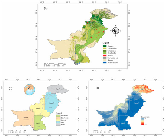
Figure 1.
Geographical location of the study region. (a) Land cover types in Pakistan during 2019, derived from the MODIS MCD12Q1 Version 6 data product. (b) Five homogeneous and contiguous regions were developed, which are similar to the climatic regions developed by [13]. (c) Digital Elevation Model based on the ASTER 30 m Digital Elevation Model.
2.2. The FY-3D MERSI-II Data
FY-3D MERSI-II satellite data have very high potential usages for various research fields. Climate change, water vapor estimation, numerical weather forecast, space weather prediction, and ecosystem monitoring are just a few of the many applications for the FY-3D MERSI-II satellite data [25]. The above-mentioned applications would benefit from a method that accurately and quickly retrieves LST from the MERSI-II data (i.e., the TFSW algorithm) [7]. Table 1 and Figure 2 compare the required bands of MERSI-II with the corresponding ones of MODIS for LST estimation. MERSI-II is similar to MODIS in certain ways, particularly in terms of wavelength frequency and band parameters. MERSI-II is a modified version of the first-generation same track type satellite sensors in terms of data quality, band number, resolution, and other factors, in order to increase the detection range for various application areas. According to the TFSW algorithm characteristics, Bands 24 and 25 of MERSI-II are selected for LST estimation. The spectral response function of the MODIS (Band 31/32) and MERSI-II (Band 24/25) TIR bands are shown in Figure 2. From Table 1 and Figure 2, it can be clearly observed that the TIR band range of MERSI-II and MODIS is similar, and that the central wavelength is also similar to some extent. It is also verified that the MODIS data can be used for validation purposes. This study uses FY-3D MERSI-II Level-1B radiance data downloaded from the Fengyun Satellite Data Archiving Portal (http://satellite.nsmc.org.cn) (accessed on 20 April 2022).

Table 1.
FY-3D sensor characteristics that correspond to the MODIS TIR Bands are commonly used for retrieving land surface temperature.

Figure 2.
Spectral response functions of the MERSI-II and MODIS TIR channels.
2.3. The MODIS Data
Terra and Aqua are the sensors of the MODIS satellite, which collects data at a high frequency of two observations per day, accessed from portal (https://lpdaac.usgs.gov/products/mod11a1v061/) (accessed on 6 May 2022). Its LST products are among the most mature methods, and have been evaluated in numerous previous studies [26,27,28,29,30]. As we know, the MERSI-II was launched in recent years, and it provide data from 2018, which is not enough to understand the spatiotemporal variations of LST in a broader way at historical scales. Therefore, the MODIS 1 km LST products (MYD11A1 and MYD21A1) were used in this study for two purposes, the first being to cross-validate the LST retrieved from MERSI-II, and second, to evaluate the long-term LST trend for the period between 2005 and 2018. We chose observations from the Terra satellite that provide an estimate of the daily maximum and minimum temperatures. The LST observations were monitored carefully for visual interpretation to ensure that the average LST pixels were within the acceptable quality range for accurate analysis.
3. Materials and Methods
3.1. The TFSW Algorithm for LST Retrieval
The radiance is measured at the top of the atmosphere (TOA) in the TIR bands as follows, using the radiative transfer theory, assuming a cloud-free atmosphere in thermodynamic equilibrium [31]:
where Bi is the Plank function, Ti is the brightness temperature (BT), εi is the emissivity, Bi(Ts) is the radiance measured when the surface is a blackbody with a surface temperature of Ts, τi is the total atmospheric transmittance (AT), R↑ atmi is the upwelling radiance, and R↓ atmi is the downwelling radiance. The SW technique represents LST as a straightforward linear or nonlinear combination of the TOA brightness temperatures of two adjacent bands based on differential water vapor absorption in two neighboring TIR bands. This method does not require real-time atmospheric profiles [32]. Due to its practicality and efficiency, the SW algorithm is therefore frequently utilized in LST retrieval. The SW algorithm is one of the most widely utilized delegate algorithms that has produced various satellite LST products [33]. Wan [34] developed a more sophisticated generalized split window approach for the MODIS Collection 6 LST product.
Bi(Ti) = εiBi(Ts)τi + R↑ atmi + (1 − εi)R↓ atmiτi
Qin et al. [35] developed a TFSW algorithm for LST retrieval from the NOAA-AVHRR Bands 4 and 5, completely based on the mathematical derivation from the thermal radiance transfer equation. The TFSW algorithm uses a series of linear combinations of two apparent temperatures, the corresponding band-averaged emissivity, and transmittance, to estimate the MERSI-II LST as follows:
where Ts is the retrieved FY-3D MERSI-II LST (K), A0, A1, and A2 are the internal parameters, Ti is the brightness temperature (BT) of the FY-3D MERSI-II TIR band i (i = 24 or 25), τi is the AT for band i, εi is Land Surface Emissivity (LSE) for the band i, and ai, and bi are the constants for the band i. The constants for the two FY-3D MERSI-II TIR bands are determined as follows:
where Li is the derivative of the Planck function Bi (T) with temperature T for the FY-3D MERSI-II TIR band i, which could be approximated as [Bi (T + ∆T) − Bi (T)]/∆T for the determination of the constants as follows:
where ai and bi are the constants for the band i. It assumes Li with T from −50 °C to 50 °C for the two FY-3D MERSI-II TIR bands, and then the constants are finally determined as follows: a24 = −53.477, b24 = 0.3951; a25 = −57.087, and b25 = 0.4292. With these constants, it is able to retrieve LST from the FY-3D MERSI-II TIR bands under the conditions where the two required parameters AT and LSE are estimated. This algorithm is just for the cloud-free pixels’ LST estimation. Thus, the cloud detection product was used as the cloud mask layer to filter clear-sky pixels.
Ts =A0 + A1T24 − A2T25
A0 = a24[D25(1 − C24 − D24)/(C24D25 − C25D24)] − a25[D24 (1 − C25 − D25)/(C24D25 − C25D24)]
A1 = 1 + D24/(C24D25 − C25D24) + b24 [D25 (1 − C24 − D24)/(C24D25 − C25D24)]
A2 = D24/(C24D25 − C25D24) + b25[D24 (1 − C25 − D25)/(C24D25 − C25D24)]
C24 = ε24τ24
D24 = [1 − τ24] [1 + (1 − ε24) τ24]
C25 = ε25τ25
D25= [1 − τ25] [1 + (1 − ε25) τ25]
Li = Bi (T)/[∂Bi (T)/∂T] ≈ Bi (T)/{[Bi (T + ∆T) − Bi (T)]/∆T}
Li = ai + biTi
The LST retrieval algorithm (Equation (2) requires three major parts: (1) radiation calibration for the computation of brightness temperature, (2) water vapor content, and (3) atmospheric transmittance based on water vapor. A more detailed description of these parameters and its calculation methodology required for the improved TFSW algorithm can be found in [7,25].
3.2. Calculation of the LSE for FY-3D MERSI-II
After the emissivity of bare soil εsi for the FY-3D MERSI-II TIR bands 24 and 25 were calculated from the bare soil emissivity of the Advanced Spaceborne Thermal Emission and Reflection Radiometer (ASTER) TIR bands 13 εs13 and 14 εs14, the land surface emissivity εi of each FY-3D MERSI-II pixel could be further estimated with the mixed pixel emissivity model, the FY-3D MERSI-II vegetation emissivity εvi, and the corresponding vegetation cover fraction Pv had been calculated from the FY-3D MERSI-II NDVI data. According to Du et al. [7] the emissivity for the FY-3D MERSI-II data can be calculated as follows:
where εi is the LSE of the FY-3D MERSI-II data and εvi is the vegetation emissivity used to estimate the LSE for FY-3D MERSI-II TIR bands 24 and 25, which has the value as εv24 = 0.982 and εv25 = 0.984, respectively; εsi is the bare soil emissivity for LSE estimation. The FY-3D MERSI-II multi-year average bare soil emissivity image could be obtained from the ASTER (Global Emissivity Dataset) GED database’s mean emissivity to replace the bare soil emissivity constant usually used in the VCM method; this can represent changes in bare soil’s emissivity in space, enhancing the precision of emissivity inversion.
εi = εvi Pv + εsi (1 − Pv)
In terms of the following, LSE for a pixel can be simply understood as a weighted mix of vegetation and bare soil emissivity [36], as follows:
where εi is the emissivity, εsi and εvi represent the emissivity of bare soil and vegetation in channel i, and Pv is the proportional of vegetation, which is calculated as follows:
NDVImin represents the value of bare soil and NDVImax represents the value of vegetation.
εi = εvi Pv + εsi (1 − Pv)
Pv = [(NDVIa − NDVImin)/(NDVImax − NDVImin)]
The emissivity values of each surface type (i.e., bare soil and vegetated portion) were traditionally determined using spectral library data, which is accurate for the vegetated portion’s high and low-contrast emissivity. However, soil emissivity in the TIR bands may vary significantly due to the various mineral components, soil moisture content, and surface roughness. Therefore, it is necessary to estimate each pixel’s emissivity of the soil type component. A detailed description can be found in the works of Wang et al. [37,38], to utilize the ASTER GED Product for thermal bands.
3.3. Comparison
The correctness of the TFSW algorithm was tested using a number of statistical techniques, including the Pearson correlation coefficient (R), the root mean square deviation (RMSD), and bias. The equations for these statistical metrics are as follows:
where xi are the estimated data, yi is the MODIS LST product from the ith time, x is the overall average of the estimated data, y is the average of the MODIS data over the study period, and R is the Pearson correlation. In this scenario, R is between minus and plus 1.
where N represents the number of pixels. RMSD was performed to see how well the particular variable correlation explained the observed variance. The difference between the actual and estimated variables is referred to as bias.
3.4. Linear Analysis of LST Variation in Pakistan
Monthly, seasonal, and yearly data were processed from the daily data to identify LST fluctuations in Pakistan. The following equation was used to calculate the mean temperatures at various temporal scales:
where LSTm represents the mean of the month, season, or year Ti satellite overpass times, and N is the number of times. We comprehensively analyzed the spatial variation of LST through the annual, seasonal, and monthly variation rates of LST, and focused on the regions with an obvious variation trend from the 2018 to 2021 years’ data. In this study, the spring (March to May), summer (June to August), autumn (September to November), and winter (December to February) seasons were utilized to classify Pakistan’s seasons into four categories. The linear monthly, seasonally, and yearly changes of temperature were calculated as:
3.5. Trend Analysis
The next step was to compute the spatiotemporal LST distribution after comparing the data’s quality. An examination of the trends using statistics was then carried out. Many statistical trend analysis techniques, including linear trend analysis, polynomial trend analysis, harmonic trend analysis, and Mann–Kendall (MK) trend analysis, have already been employed in related investigations [39]. In order to evaluate the statistical significance of the trends and to precisely estimate the amplitude of the changes in LST, the Sen’s slope estimator and the non-parametric MK methods were utilized in this study. Numerous research projects have used the non-parametric MK test because it does not rely on any assumptions about the distribution of the data or the linearity of the trend [40]. The alternative hypothesis indicates that there is a monotonic decreasing or increasing trend, whereas the null hypothesis in the calculation of this test asserts that there is no trend in LST data over time. The equations to use the MK test are as follows:
Xj and Xk are two consecutive data values in an n-dimensional data set. The term “sgn” represent sign function. For a normal distribution, E(S) = 0 with the variance, and the S statistic behaves roughly the same. Here, q is the total number of affiliated groups in the data set, and tp is the number of input values contained within the p-th affiliated group. By utilizing above equations, Zmk is calculated as follows:
A statistically reliable trend identification tool is Zmk. A Zmk positive sign indicates an upward trend, while a Zmk negative sign indicates a downward trend. The null hypothesis is rejected if the absolute value of Zmk > Z1/2, where Z1/2 is obtained from the normal cumulative distribution tables.
The estimator of Sen [41], which is defined by Equations (24) and (25), was used to calculate the real slope of an existing trend.
There will be N = n (n − 1)/2 slope Qi estimations if the time series has n Xj values. The median of these N values of Qi is Sen’s slope estimator which calculated as follows:
3.6. Procedure of the Study
Figure 3 shows the research procedure and technical methods, including the detailed steps for retrieving LST from the MERSI-II data. The following are the steps that this study takes as its main approach: We start by obtaining Level 1 radiance data from the FY-3D satellite data portal. Second, we estimate the LST and its required parameters of the TFSW algorithm. Third, we conducted a cross-validation analysis on the retrieved LST to determine the algorithm’s applicability and usefulness. Finally, the application of the algorithm was applied for the detailed spatial and temporal analyses of LST for Pakistan.
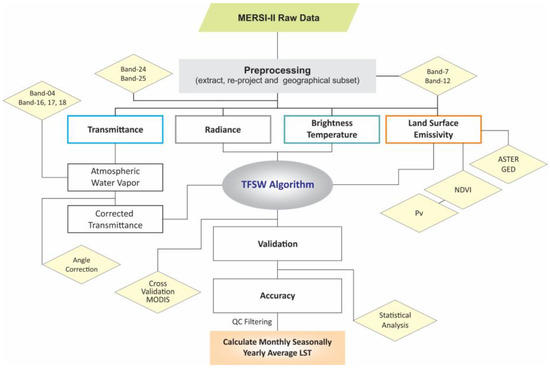
Figure 3.
The framework depicting the phases required for LST estimation and spatiotemporal analysis.
4. Results
4.1. Cross-Validation between MERSI-II, and MYD11 and MYD21 MODIS LST Products
The validation of LST based on the measured data is a difficult task. Wan et al. [42] put his extensive efforts toward correctly verifying the MODIS LST products with the measured data. His findings reveal that the MODIS MYD11A1 LST product in the experimental area are accurate to within 1 °C. Hence, for relative error analysis, we used the MYD11A1 and MYD21A1 LST products, and the MERSI-II-estimated LST data. The LST of two different raster datasets (MYD11A1/MYD21A1 and MERSI-II) were extracted by using the shapefiles of different sub-regions over the study area; the results of differences in LST between the MERSI-II, and the MODIS MYD11A1 and MYD21A1 products are shown in Figure 4 and Figure 5.

Figure 4.
Cross-validation errors between LSTs of MERSI-II, and MODIS (a) MYD11A1 and (b) MYD21A1 LST products over five sub-regions of Pakistan.
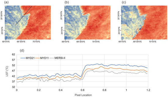
Figure 5.
Spatial distribution of (a) MYD11A1, (b) MYD21A1, and (c) MERSI-II LST data. The dotted line represents the profile extraction location. (d) Latitudinal profile of three different LST data.
It was observed that the RMSD between MERSI-II, MYD11A1 and MYD21A1 ranged from 1.71 to 5.31 °C throughout the year, over the sub-regions of Pakistan. The highest RMSDs were recorded in region IV in both the LST products, and they were the lowest in region V, which was an average of annual record. Regarding bias, region II showed the highest negative trend when compared to MYD11A1, and the highest positive trend of bias were observed in region IV in a comparison of both products. The highest error in RMSE was possibly due to various reasons, such as heterogeneous surfaces producing larger errors due to uneven surface features. The LST retrieved from remote sensing data was the instantaneous LST at the moment of sensor imaging. The imaging time of the original images used for the retrieval of MERSI-II LST and MYD11AI and MYD21A1 LST differed, and the sensor calibration accuracy also differed. Thus, the LST results of the same area slightly differed due to retrieval using different remote sensing data sources.
The LST distributions in all datasets were almost same under clear sky conditions (as shown in Figure 5), with only minor deviations being observed in MERSI-II, possibly the stripe noise problem of the sensor. According to the latitudinal profile, it can observed that the LST of MERSI-II was close the MYD11A1 LST product as compared to the MYD21A1, and the overall RMSD errors were also smaller when compared with the MYD11A1 product. However, the image acquisition times of both sensors were similar to some extent, but not identical, and the MODIS LST product itself contained some minor errors when compared to the ground data. In this regard, when we compared MERSI-II’s retrieved LST with the MODIS LSTs products, the results are merely a spatial analysis of the LSTs, and relative errors are not perfectly precise.
4.2. Spatial Distribution of the Annual Mean LST
The spatial distribution of the annual mean LSTs of Pakistan is almost the same in 2018 and 2021; small variations were observed, as the time span (i.e., 4 years) is not very long. The annual mean LST of Pakistan ranged between −15 and 55 °C (Figure 6). A bar chart was developed to demonstrate the linear change of the annual mean LST between 2018 and 2021 over the sub-regions of the study area, and differential variations in pixel scale between two raster datasets were performed to validate substantial upward or downward variations. It was observed from the annual mean LST that 2018 was the coldest year (33.63 °C), while 2021 was the warmest (34.42 °C). The temperature difference between the coldest and warmest years was about 0.79 °C.

Figure 6.
Spatial distribution of annual mean LST in Pakistan. (a–d) Mean LSTs of 2018, 2019, 2020, and 2021. (e) LST difference between 2018 and 2021 on spatial scales. (f) Bar chart for mean LST difference for sub-regions of Pakistan.
When the geographical characteristics of the location are considered, it was discovered that the low elevation increased thermal insulation, resulting in a greater LST. In terms of geographical cover, Pakistan’s greatest desert, Thar, is located around the Indian border in the southeast. The desert covers an area of 175,000 square kilometers, including significant regions of Pakistan and India. It is Pakistan’s largest desert, and Asia’s only subtropical desert that absorbs sun radiation. During the analysis of the spatial distribution of annual mean LST throughout the sub-regions, the region II exhibits the highest annual mean LST, varying between 41 and 42 °C. The same scenario was observed in region I. Due to various geographical surface features, region III is slightly different, with a mean LST of 36 °C. Region IV is the transitional zone between the temperate and severe climate zones; the annual mean LST of this region is around 31 °C, but it varies greatly across the landscape. The lowest LST values were discovered in region V, which were decreased by up to −22 °C; however, in the southern parts of this region, the temperature was increased up to 39 °C.
We calculated the linear mean LST difference by subtracting the data values from two raster datasets. The warming and cooling of the LST trend were shown by positive and negative values. Figure 6e depicts the results after subtracting the initial and final raster data values at the pixel scale, while Figure 6f depicts the mean annual difference. Northern Pakistan is cooled more than Southern Pakistan, resulting in the highest cooling effect in the north and a moderate cooling effect in the south. However, many locations of region IV have an LST difference of less than 0 °C, which is primarily cooling. The largest warming trend (0.68 °C) was identified in region I, whereas the minimum warming trend (0.32 °C) was recorded in region IV. The explanation for the cooling trend in region V is unknown, possibly due to the missing data of thin clouds. The warming tendencies in regions I and II, on the other hand, are due to changes in their geographical land cover types.
4.3. Trend Analysis of the Annual Mean LST
The MK trend test results (Table 2) of LST for the Pakistan showed positive and negative trends during the time span of 2018 to 2021. In this section, the positive values represent increasing, and the negative values represent decreasing trends in the regions, the p-value decides the level of significance, and the slope indicates the magnitude of LST. The highest increasing trend (0.019 °C/year) at a 10% level of significance was observed in region V. The other regions also showed increasing trends, but these were insignificant. The lowest decreasing trend was observed in region I at a 5% level of significance, with a magnitude of −0.013 °C/year, which was lowest among the other regions. However, as evidenced from the minimum and maximum values of Table 2 and Figure 7, there are lot of areas that experience significant increasing and decreasing trends, but these are very small in area. Figure 7 shows the spatial distribution of the MK parameters. The most important significant trends can be observed from Figure 7d, which shows increasing trends in the northern areas and decreasing in the southern areas. The slope of the LST per year throughout the study region ranged between −0.013 and 0.019 °C/Year.
Table 2.
MK trend test (Z) statistics, Sen’s slope, and p value for the LST trends analysis.

Figure 7.
Spatial distribution of (a) Mann–Kendall, (b) Sen’s Slope, (c) Level of Significance (p-value), (d) Statistically significant data at 99% level of confidence.
4.4. Spatial Distribution of Seasonal LST and Trend Analysis
The spatial distribution of the seasonal mean LST rises with decreasing latitude, similar to the yearly mean LST, with low values in the northern and high values in the southern regions of the country. However, there are differences between each seasonal dataset. Because the Earth’s axis is tilted relative to the orbital plane, the solar elevation angle fluctuates throughout the year, making winter cold and summer hot. To further reveal the LST changes, seasonal means were processed from the daily averages of the LST data to calculate the trend analysis through the MK test, along with the slope (Table 3). Based on the classification of the four seasons throughout the study region, seasonal variation has an important effect on LST across Pakistan.
Table 3.
The mean LST difference along with standard deviation at seasonal scales.
The results of the spatial–temporal changes of LST over different seasons are given in Figure 8. The overall mean of the seasonal LST varies from −26 to 60 °C throughout Pakistan. During the overall seasons, the highest LSTs were observed in region II, particularly in the summer season, which reached up to 50.86 °C, which is the highest among the other regions and seasons. This result can be attributable to the fact that the annual rainfall is below average. Furthermore, barren ground, which is more susceptible to LST changes than vegetation-covered land, could be another factor for the rise in LST. Similarly, the lowest LST were observed in region V in all seasons, especially in the winter season, where the mean LSTs of this region were decreased up to −9.7 °C; there are some places that contain higher LSTs, especially in the southern parts of that region. During the autumn and spring seasons, similar trends were observed, followed by winter and summer, especially in regions II and V. The mean LSTs of the spring and autumn season reached up to 42 and 46 °C, respectively, in region II.

Figure 8.
Spatial distribution of seasonal mean LSTs between 2018 and 2021 in Pakistan. (a) Spring, (b) summer, (c) winter, (d) autumn.
The results of the trend analysis and Sen’s slope at seasonal scales were presented in Table 3. The highest increasing trend (0.20 °C) at a 1% level of significance (p < 0.01) was observed in region V during the summer season; there were also increasing events in other seasons, except for the spring season. Another warming event was observed in region II during the summer season. Contrary, the highest cooling trend was observed in region I during the autumn season (−0.08 °C) which is highest among all seasons and regions. The factors attributed to this cooling trend could be the Khirthar mountainous regions, which cover an area of about 9000 square kilometers, with the highest peak of 2260 m. Due the high altitude, the LST of this region does not significantly increase in 2018 and 2021. When we investigate the low altitude/flat surfaces, the only region IV is a region where the change rate of LST significantly increases significantly in the summer seasons throughout the season, and the highest heating trend has a magnitude of 0.08 °C.
4.5. Monthly Average Change Analysis
Figure 9 and Figure 10 provide the overall monthly LST spatial distribution and the difference of LST between 2018 and 2021. The spatial variation of LST can easily determined using the monthly datasets of FY-3D MERSI-II data, and the LSTs were gradually increased from January, reached their peak in June to August, and then they declined throughout Pakistan. The highest mean LSTs during 2018 and 2021 were recorded in June (43.6 °C), and the lowest in January (14.3 °C). In terms of sub-regions, the monthly LST variations were followed by annual and seasonal trends. Throughout the monthly analysis, region II contained the highest LST and region V, the lowest; these highest and lowest LST values possibly differed due to the latitudinal change and the geographical land cover types. According to Figure 10, a warming trend were observed in region II throughout the monthly results except for the January (−0.93) and December (−0.83) months, which resulted in that the LSTs in 2021 were higher than 2018. However, region V does not follow decreasing or increasing trends; there are many cooling and warming trends observed because of the surface heterogeneity and snow cover. Regarding region IV, there are some events in the monthly analysis that follow the cooling trends compared to the 2018 and 2021, but they are not a priority for discussion. The monthly change analysis was calculated by subtracting the monthly rasters between 2018 and 2021. The MK trends analysis was never applied over a monthly basis due to the limited availability of temporal data.
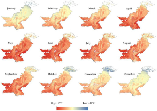
Figure 9.
Spatial distribution of mean LSTs of 2018 and 2021 at monthly scales in Pakistan.

Figure 10.
The monthly mean variations of LST over different sub-regions of Pakistan during 2018 to 2021.
4.6. Long-Term Interannual Variations of LST
Long-term interannual variations of LST are crucial for the investigation of the LST warming and cooling trends. From the above analyses, we observed that the FY-3D MERSI-II data and the TFSW algorithm performed well for understanding the LST variations throughout Pakistan in 2018 and 2021; the validations results also supported their usefulness. However, the FY-3D MERSI-II is a recently launched satellite; to understand the spatial–temporal variations of LSTs to a broad extent requires the crucial contribution of historical data (i.e., over 10 years). The MODIS MYD11A1 product is fully mature and is a widely used LST product at global scales. To understand the interannual LST variations in Pakistan, we used MODIS LST data from 2005 to 2018.
The long-term spatial patterns of LST (2005 and 2018) are like the above mentioned annual mean LST trends of MERSI-II. The long-term annual mean LST varies from −29 to 55 °C across Pakistan (Figure 11). The spatial–temporal variation between 14 annual LST raster datasets were performed to demonstrate the change that occurred in Pakistan through MK trend analysis and Sen’s slope estimator, and a line chart was introduced to show a mean LST and histogram for an individual year. Figure 11 shows how the mean annual LST (°C) varied across the country over this time. The coldest year (34.16 °C) was 2012, and the warmest year (35.53 °C) was 2016. The coldest and warmest years were separated by about 1.37 °C. Similar to the MERSI-II annual mean LST, with increasing latitude, the MODIS annual LST likewise decreased; it had low values in the northern areas and high values in the southern areas. The MODIS annual LST also decreased with increasing latitude: it had low values in the northern regions and high values in the southern regions. The LST trend for every year (from 2005 to 2018) followed this increasing and decreasing trend throughout Pakistan.
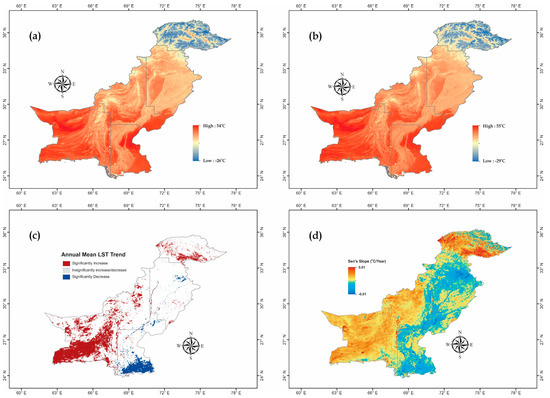
Figure 11.
The spatial distribution of the mean LSTs and trend variables. (a) Annual LST in 2005, (b) annual LST in 2018, (c,d) significant increase and decrease along with Sen’s slope from 2005 to 2018.
The MK trend results show almost similar trends, as we have seen for MERSI-II, but the slopes per year of the annual mean LST are very small, as displayed in Figure 11c,d. The slopes were found to be between −0.01 and 0.01 °C/year throughout Pakistan. In regions II and V, there was a considerable increasing tendency at a 5% level of significance, with a slope of 0.0046 and 0.0047 °C/year. Region I exhibited a considerable decreasing trend of roughly −0.0024 °C/year. The various increasing and decreasing trends in other regions of the study are insignificant. The results of the long-term interannual variations of MODIS are consistent with an annual mean LST of the FY-3D MERSI-II data. The positive slope and the positive correlation of the LSTs in regions I and II are directly related to their geographical land cover types, which have already been discussed in the above sections.
The greatest interannual differences were found in regions I, II, and V. In contrast, there was less interannual variability in region IV. The greatest interannual disparities may be due to changes in the surfaces’ vegetation cover. This is because the thermal characteristics of the Earth’s surfaces with high vegetation cover differ from those of the Earth’s surface with low vegetation cover. The increase in vegetation cover helps to increase the soil moisture content, which helps to prevent soil erosion and desertification. Surface temperatures in the equatorial and temperate regions are often higher in areas with low vegetation cover than in areas with high vegetation cover.
Furthermore, Figure 12 shows the mean LST of individual year and histogram of years between 2005 and 2018, and it was observed that the LST trend was almost same, with small deviations throughout the years. The country’s maximum areas of LST were approximately 28 to 50 °C.

Figure 12.
(a,b) Interannual Mean LST, including its frequency histogram for the years of 2005 to 2018 throughout the Pakistan.
5. Discussion
The TFSW algorithm’s accuracy and adaptability were evaluated by comparing the LSTs of MERSI-II with MYD11A1 and MYD21A1 LST over various study regions. The LST difference ranged between 1.74 and 5.2 °C over the different regions of Pakistan. The MERSI-II LST performs well with the MODIS MYD11A1 LST product; the error range was between 1.94 and 4.27 °C, which is slightly higher but close to the several published studies [7,12,43,44]. The regions that experience the highest LST difference could possibly be due to the surface types, and the presence of humidity produces larger uncertainties [44]. Regarding the LST distribution, the highest LSTs were observed in the southern areas, and the lowest in the northern areas. The amount of solar radiation energy received by the ground decreases as latitude increases. As a result, the annual mean LST distribution pattern is characterized by high values in the southern regions and low values in the northern parts. There are, however, some locations that do not follow this trend. Because the areas where the Indus River flows, particularly in the country’s central lower latitudes, are largely productive, resulting in moderate heat preservation on the ground, it has a lower annual mean LST than its nearby places. The great mountainous region occurred in northern areas, which is Pakistan’s greatest altitude region, with an average elevation of above 5000 m. Because the location is at a high elevation, the air near the surface is thin, resulting in poor heat retention on the ground and a lower annual mean LST than in other parts of the country. According to the MK trend analysis, the highest warming impacts (0.019 °C/Year) were noted in the northern areas, with a high level of significance. This scenario was also observed in seasonal trends as well as long-term analysis trends. The reasons for this increasing are possibly the impacts of global warming and climate change [45]. By taking into account meteorological data from two sites, Ali et al. [46] looked into changes in temperature in the Upper Indus Basin. In line with this investigation, they observed that the mean temperature increased by 0.63 °C in Skardu, whereas it recently declined by 0.137 °C in Gilgit. The source of the decreasing trends in southern region I is unknown. There are strong increasing trends through seasonal and monthly analyses in regions I and II. The lack of rain and growing drought have had a substantial impact on the temperature fluctuations of Southern Pakistan. The hottest temperatures have had a significant detrimental influence on Pakistan’s primary crops, such as wheat and cotton. Early in the spring season, a minor heat wave (13 days over the usual 2–3 °C temperatures) resulted in a 28 percent decline in wheat grain yield.
When evaluating the results, it is important to take into account the limitations of the current study. The remote sensing data are not enough to obtain precise LST trends. However, the various factors that affect LSTs are still not considered in this study, such as elevation, land cover types, and water vapor; even the NDVI has a considerable influence on LSTs [47]. To ensure the reliability of the results, future studies should employ LST data, including elevation, land cover types, water vapor, etc.
6. Conclusions
During MERSI-II’s operation in orbit, China’s satellite remote sensing observation capabilities were increasing. This sensor is the first imaging instrument in the world that can acquire thermal infrared data with a spatial resolution of 250 m and 1000 m. The MERSI-II data can be used to precisely recover the land surface temperature using the recently developed TFSW algorithm. The Moderate Spectral Resolution Atmospheric Transmittance Model simulation dataset served as the source for the SW algorithm coefficients (MODTRAN). In a comparison of the retrieved LST and the MODIS MYD11A1 and MYD21A1 LST product, it was found that the MERSI-II LST is more reliable and achieves a better accuracy in a comparison with MYD11A1.
In order to study the spatiotemporal changes in LSTs, the FY-3D MERSI-II LST data have never before been employed in Pakistan on this scale. MK trend analysis and Sen’s slope estimator were applied to identify significant changes. Due to the limited availability of the MERSI-II data (i.e., 4 years), the MODIS MYD11AI product was utilized to understand the interannual variations of LSTs in Pakistan. Considering both satellites, these conclusions were noticed: (1) The annual mean LST in Pakistan often follows a pattern with high values in the southern parts and low values in the northern regions, which is consistent with the rule that solar radiation intensity decreases with increasing latitude. However, the spatial distribution of LST is also influenced by elevation and the types of land cover. (2) The spatial distribution of the annual mean LST was almost similar during the study period. The trend analysis shows that the northern areas (region v) have increasing LST trends. The LST changed on average by 0.019 °C/year, increasing in the northern parts and decreasing by 0.013 °C/Year in the southern regions. With regard to the sub-regions, a maximum LST were observed in region II, and a greater warming trend were also observed in this region, with a rapidly increasing rate of 0.0046 °C/year when utilizing long-term data, with the p-value also being consistent with the slope.
Due to the influence of the stripe noise in the MERSI-II TIR pictures, the validation of the recovered LST utilized may be a little inaccurate in comparison. Even yet, some in-depth and in situ confirmations are still needed. In order to fully utilize the MERSI-II TIR photos, further work should concentrate on stripe noise removal, as well as confirmation with ground-based stations, particularly in the American regions. Additionally, LST variations are crucial elements that affect and that restrain climate change in various ways. Governmental institutions and groups that are concerned with the environment must therefore pay close attention to changes in the LST, in order to define climate change.
Author Contributions
Conceptualization, B.A. and Z.Q.; methodology, B.A.; software, J.F.; validation, B.A., W.D. and S.L.; formal analysis, B.A.; investigation, Z.Q.; resources, C.Z.; data curation, W.D.; writing—original draft preparation, B.A. and Z.Q.; writing—review and editing, W.D., Z.Q. and C.Z.; visualization, B.A.; supervision, Z.Q. and J.F.; project administration, Z.Q.; funding acquisition, Z.Q. All authors have read and agreed to the published version of the manuscript.
Funding
This study was supported by the National Key Research and Development Program of China (Grant No.: 2019YFE0127600), and the National Natural Science Foundation of China (Grant No.: 41771406, 41921001).
Institutional Review Board Statement
Not applicable.
Informed Consent Statement
Not applicable.
Conflicts of Interest
The authors declare no conflict of interest. The funders had no role in the design of the study; in the collection, analyses, or interpretation of data; in the writing of the manuscript, or in the decision to publish the results.
References
- Yao, R.; Wang, L.; Huang, X.; Gong, W.; Xia, X. Greening in Rural Areas Increases the Surface Urban Heat Island Intensity. Geophys. Res. Lett. 2019, 46, 2204–2212. [Google Scholar] [CrossRef]
- Zhou, C.; Wang, K. Land Surface Temperature over Global Deserts: Means, Variability, and Trends. J. Geophys. Res. Atmos. 2016, 121, 14344–14357. [Google Scholar] [CrossRef]
- Bhattarai, N.; Mallick, K.; Stuart, J.; Vishwakarma, B.D.; Niraula, R.; Sen, S.; Jain, M. An Automated Multi-Model Evapotranspiration Mapping Framework Using Remotely Sensed and Reanalysis Data. Remote Sens. Environ. 2019, 229, 69–92. [Google Scholar] [CrossRef]
- Lu, N.; Liang, S.; Huang, G.; Qin, J.; Yao, L.; Wang, D.; Yang, K. Hierarchical Bayesian Space-Time Estimation of Monthly Maximum and Minimum Surface Air Temperature. Remote Sens. Environ. 2018, 211, 48–58. [Google Scholar] [CrossRef]
- Randazzo, G.; Cascio, M.; Fontana, M.; Gregorio, F.; Lanza, S.; Muzirafuti, A. Mapping of Sicilian Pocket Beaches Land Use/Land Cover with Sentinel-2 Imagery: A Case Study of Messina Province. Land 2021, 10, 678. [Google Scholar] [CrossRef]
- Randazzo, G.; Italiano, F.; Micallef, A.; Tomasello, A.; Cassetti, F.P.; Zammit, A.; D’Amico, S.; Saliba, O.; Cascio, M.; Cavallaro, F.; et al. WebGIS Implementation for Dynamic Mapping and Visualization of Coastal Geospatial Data: A Case Study of BESS Project. Appl. Sci. 2021, 11, 8233. [Google Scholar] [CrossRef]
- Du, W.; Qin, Z.; Fan, J.; Zhao, C.; Huang, Q.; Cao, K.; Abbasi, B. Land Surface Temperature Retrieval from Fengyun-3d Medium Resolution Spectral Imager Ii (Fy-3d Mersi-Ii) Data with the Improved Two-Factor Split-Window Algorithm. Remote Sens. 2021, 13, 72. [Google Scholar] [CrossRef]
- Tang, K.; Zhu, H.; Ni, P.; Li, R.; Fan, C. Retrieving Land Surface Temperature from Chinese FY-3D MERSI-2 Data Using an Operational Split Window Algorithm. IEEE J. Sel. Top. Appl. Earth Obs. Remote Sens. 2021, 14, 6639–6651. [Google Scholar] [CrossRef]
- Wang, H.; Mao, K.; Mu, F.; Shi, J.; Yang, J.; Li, Z.; Qin, Z. A Split Window Algorithm for Retrieving Land Surface Temperature from FY-3D MERSI-2 Data. Remote Sens. 2019, 11, 2083. [Google Scholar] [CrossRef]
- Jin, M.; Li, J.; Wang, C.; Shang, R. A Practical Split-Window Algorithm for Retrieving Land Surface Temperature from Landsat-8 Data and a Case Study of an Urban Area in China. Remote Sens. 2015, 7, 4371–4390. [Google Scholar] [CrossRef]
- Ndossi, M.; Avdan, U. Inversion of Land Surface Temperature (LST) Using Terra ASTER Data: A Comparison of Three Algorithms. Remote Sens. 2016, 8, 993. [Google Scholar] [CrossRef]
- Li, Z.-L.; Tang, B.-H.; Wu, H.; Ren, H.; Yan, G.; Wan, Z.; Trigo, I.F.; Sobrino, J.A. Satellite-Derived Land Surface Temperature: Current Status and Perspectives. Remote Sens. Environ. 2013, 131, 14–37. [Google Scholar] [CrossRef]
- Jamro, S.; Dars, G.H.; Ansari, K.; Krakauer, N.Y. Spatio-Temporal Variability of Drought in Pakistan Using Standardized Precipitation Evapotranspiration Index. Appl. Sci. 2019, 9, 4588. [Google Scholar] [CrossRef]
- Haroon, M.A.; Zhang, J.; Yao, F. Drought Monitoring and Performance Evaluation of MODIS-Based Drought Severity Index (DSI) over Pakistan. Nat. Hazards 2016, 84, 1349–1366. [Google Scholar] [CrossRef]
- Adnan, S.; Ullah, K.; Gao, S.; Khosa, A.H.; Wang, Z. Shifting of Agro-Climatic Zones, Their Drought Vulnerability, and Precipitation and Temperature Trends in Pakistan. Int. J. Climatol. 2017, 37, 529–543. [Google Scholar] [CrossRef]
- Afzaal, M.; Haroon, M.A. Interdecadal Oscillations and the Warming Trend in the Area-Weighted Annual Mean Temperature of Pakistan. Pakistan J. Meteorol. 2009, 6, 13–19. [Google Scholar]
- Mumtaz, F.; Tao, Y.; De Leeuw, G.; Zhao, L.; Fan, C.; Elnashar, A.; Bashir, B.; Wang, G.; Li, L.L.; Naeem, S.; et al. Modeling Spatio-Temporal Land Transformation and Its Associated Impacts on Land Surface Temperature (LST). Remote Sens. 2020, 12, 2987. [Google Scholar] [CrossRef]
- Arshad, A.; Zhang, W.; Zaman, M.A.; Dilawar, A.; Sajid, Z. Monitoring the Impacts of Spatio-Temporal Land-Use Changes on the Regional Climate of City Faisalabad, Pakistan. Ann. GIS 2018, 25, 57–70. [Google Scholar] [CrossRef]
- Saleem, M.S.; Ahmad, S.R.; Shafiq-Ur-Rehman; Javed, M.A. Impact Assessment of Urban Development Patterns on Land Surface Temperature by Using Remote Sensing Techniques: A Case Study of Lahore, Faisalabad and Multan District. Environ. Sci. Pollut. Res. 2020, 27, 39865–39878. [Google Scholar] [CrossRef] [PubMed]
- Pakistan Bureau of Statistics. Pakistan Statistical Year Book for Land Utilization. 2011. Available online: http://www.pbs.gov.pk/content/pakistan-statistical-year-book-2011 (accessed on 20 April 2016).
- Zaman, Q.U.; Rasul, G. Agro-Climatic Classification of Pakistan. Q. Sci. Vis. 2004, 9, 59–66. [Google Scholar]
- Mahessar, A.A.; Qureshi, A.L.; Dars, G.H.; Solangi, M.A. Climate change impacts on vulnerable Guddu and Sukkur Barrages in Indus River, Sindh. Sindh Univ. Res. J. 2017, 49, 137–142. [Google Scholar]
- Krakauer, N.Y.; Lakhankar, T.; Dars, G.H. Precipitation Trends over the Indus Basin. Climate 2019, 7, 116. [Google Scholar] [CrossRef]
- Rehman, S.; Shah, M.A. Rainfall Trends in Different Climate Zones of Pakistan. Pak. J. Meteorol. 2012, 9, 37–47. [Google Scholar]
- Abbasi, B.; Qin, Z.; Du, W.; Fan, J.; Zhao, C.; Hang, Q.; Zhao, S.; Li, S. An Algorithm to Retrieve Total Precipitable Water Vapor in the Atmosphere from FengYun 3D Medium Resolution Spectral Imager 2 (FY-3D MERSI-2) Data. Remote Sens. 2020, 12, 3469. [Google Scholar] [CrossRef]
- Hulley, G.; Veraverbeke, S.; Hook, S. Thermal-Based Techniques for Land Cover Change Detection Using a New Dynamic MODIS Multispectral Emissivity Product (MOD21). Remote Sens. Environ. 2014, 140, 755–765. [Google Scholar] [CrossRef]
- Li, H.; Sun, D.; Yu, Y.; Wang, H.; Liu, Y.; Liu, Q.; Du, Y.; Wang, H.; Cao, B. Evaluation of the VIIRS and MODIS LST Products in an Arid Area of Northwest China. Remote Sens. Environ. 2014, 142, 111–121. [Google Scholar] [CrossRef]
- Duan, S.-B.; Li, Z.-L.; Li, H.; Göttsche, F.-M.; Wu, H.; Zhao, W.; Leng, P.; Zhang, X.; Coll, C. Validation of Collection 6 MODIS Land Surface Temperature Product Using in Situ Measurements. Remote Sens. Environ. 2019, 225, 16–29. [Google Scholar] [CrossRef]
- Yao, R.; Wang, L.; Wang, S.; Wang, L.; Wei, J.; Li, J.; Yu, D. A Detailed Comparison of MYD11 and MYD21 Land Surface Temperature Products in Mainland China. Int. J. Digit. Earth 2020, 13, 1391–1407. [Google Scholar] [CrossRef]
- Li, H.; Li, R.; Yang, Y.; Cao, B.; Bian, Z.; Hu, T.; Du, Y.; Sun, L.; Liu, Q. Temperature-Based and Radiance-Based Validation of the Collection 6 MYD11 and MYD21 Land Surface Temperature Products Over Barren Surfaces in Northwestern China. IEEE Trans. Geosci. Remote Sens. 2021, 59, 1794–1807. [Google Scholar] [CrossRef]
- Li, Z.; Petitcolin, F.; Zhang, R. A Physically Based Algorithm for Land Surface Emissivity Retrieval from Combined Mid-Infrared and Thermal Infrared Data. Sci. China Ser. E Technol. Sci. 2000, 43, 23–33. [Google Scholar] [CrossRef]
- Tang, B.-H. Nonlinear Split-Window Algorithms for Estimating Land and Sea Surface Temperatures From Simulated Chinese Gaofen-5 Satellite Data. IEEE Trans. Geosci. Remote Sens. 2018, 56, 6280–6289. [Google Scholar] [CrossRef]
- Wan, Z.; Dozier, J. A Generalized Split-Window Algorithm for Retrieving Land-Surface Temperature from Space. IEEE Trans. Geosci. Remote Sens. 1996, 34, 892–905. [Google Scholar] [CrossRef]
- Wan, Z. New Refinements and Validation of the Collection-6 {MODIS} Land-Surface Temperature/Emissivity Product. Remote Sens. Environ. 2014, 140, 36–45. [Google Scholar] [CrossRef]
- Qin, Z.; Dall Olmo, G.; Karnieli, A.; Berliner, P. Derivation of Split Window Algorithm and Its Sensitivity Analysis for Retrieving Land Surface Temperature from {NOAA}-Advanced Very High Resolution Radiometer Data. J. Geophys. Res. Atmos. 2001, 106, 22655–22670. [Google Scholar] [CrossRef]
- Sobrino, J.A.; Jimenez-Muoz, J.C.; Soria, G.; Romaguera, M.; Guanter, L.; Moreno, J.; Plaza, A.; Martinez, P. Land Surface Emissivity Retrieval From Different {VNIR} and {TIR} Sensors. IEEE Trans. Geosci. Remote Sens. 2008, 46, 316–327. [Google Scholar] [CrossRef]
- Wang, H.; Yu, Y.; Yu, P.; Liu, Y. Land Surface Emissivity Product for NOAA JPSS and GOES-R Missions: Methodology and Evaluation. IEEE Trans. Geosci. Remote Sens. 2020, 58, 307–318. [Google Scholar] [CrossRef]
- Wang, C.; Duan, S.-B.; Zhang, X.; Wu, H.; Gao, M.-F.; Leng, P. An Alternative Split-Window Algorithm for Retrieving Land Surface Temperature from Visible Infrared Imaging Radiometer Suite Data. Int. J. Remote Sens. 2018, 40, 1640–1654. [Google Scholar] [CrossRef]
- Mann, H.B. Nonparametric Tests Against Trend. Econometrica 1945, 13, 245. [Google Scholar] [CrossRef]
- Sen, P.K. Estimates of the Regression Coefficient Based on Kendall’s Tau. J. Am. Stat. Assoc. 1968, 63, 1379–1389. [Google Scholar] [CrossRef]
- Gocic, M.; Trajkovic, S. Analysis of Changes in Meteorological Variables Using Mann-Kendall and Sen’s Slope Estimator Statistical Tests in Serbia. Glob. Planet. Chang. 2013, 100, 172–182. [Google Scholar] [CrossRef]
- Wan, Z.; Zhang, Y.; Zhang, Q.; Li, Z.-L. Quality Assessment and Validation of the MODIS Global Land Surface Temperature. Int. J. Remote Sens. 2004, 25, 261–274. [Google Scholar] [CrossRef]
- Hewison, T.J.; Wu, X.; Yu, F.; Tahara, Y.; Hu, X.; Kim, D.; Koenig, M. GSICS Inter-Calibration of Infrared Channels of Geostationary Imagers Using Metop/IASI. IEEE Trans. Geosci. Remote Sens. 2013, 51, 1160–1170. [Google Scholar] [CrossRef]
- Kalma, J.D.; McVicar, T.R.; McCabe, M.F. Estimating Land Surface Evaporation: A Review of Methods Using Remotely Sensed Surface Temperature Data. Surv. Geophys. 2008, 29, 421–469. [Google Scholar] [CrossRef]
- Khan, F.; Ali, S.; Mayer, C.; Ullah, H.; Muhammad, S. Climate Change and Spatio-Temporal Trend Analysis of Climate Extremes in the Homogeneous Climatic Zones of Pakistan during 1962–2019. PLoS ONE 2022, 17, e271626. [Google Scholar] [CrossRef] [PubMed]
- Ali, S.H.B.; Shafqat, M.N.; Eqani, S.A.M.A.S.; Shah, S.T.A. Trends of Climate Change in the Upper Indus Basin Region, Pakistan: Implications for Cryosphere. Environ. Monit. Assess. 2019, 191, 51. [Google Scholar] [CrossRef] [PubMed]
- Rani, S.; Mal, S. Trends in Land Surface Temperature and Its Drivers over the High Mountain Asia. Egypt. J. Remote Sens. Sp. Sci. 2022, 25, 717–729. [Google Scholar] [CrossRef]
Publisher’s Note: MDPI stays neutral with regard to jurisdictional claims in published maps and institutional affiliations. |
© 2022 by the authors. Licensee MDPI, Basel, Switzerland. This article is an open access article distributed under the terms and conditions of the Creative Commons Attribution (CC BY) license (https://creativecommons.org/licenses/by/4.0/).