

Efficient Machine Learning Models for the Uplift Behavior of Helical Anchors in Dense Sand for Wind Energy Harvesting


Abstract
1. Introduction
2. Study Background
2.1. Gradient-Boosting Decision Tree
2.1.1. Boosting
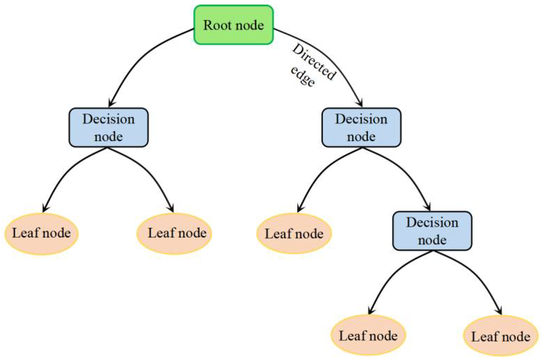
2.1.2. Classification and Regression Tree
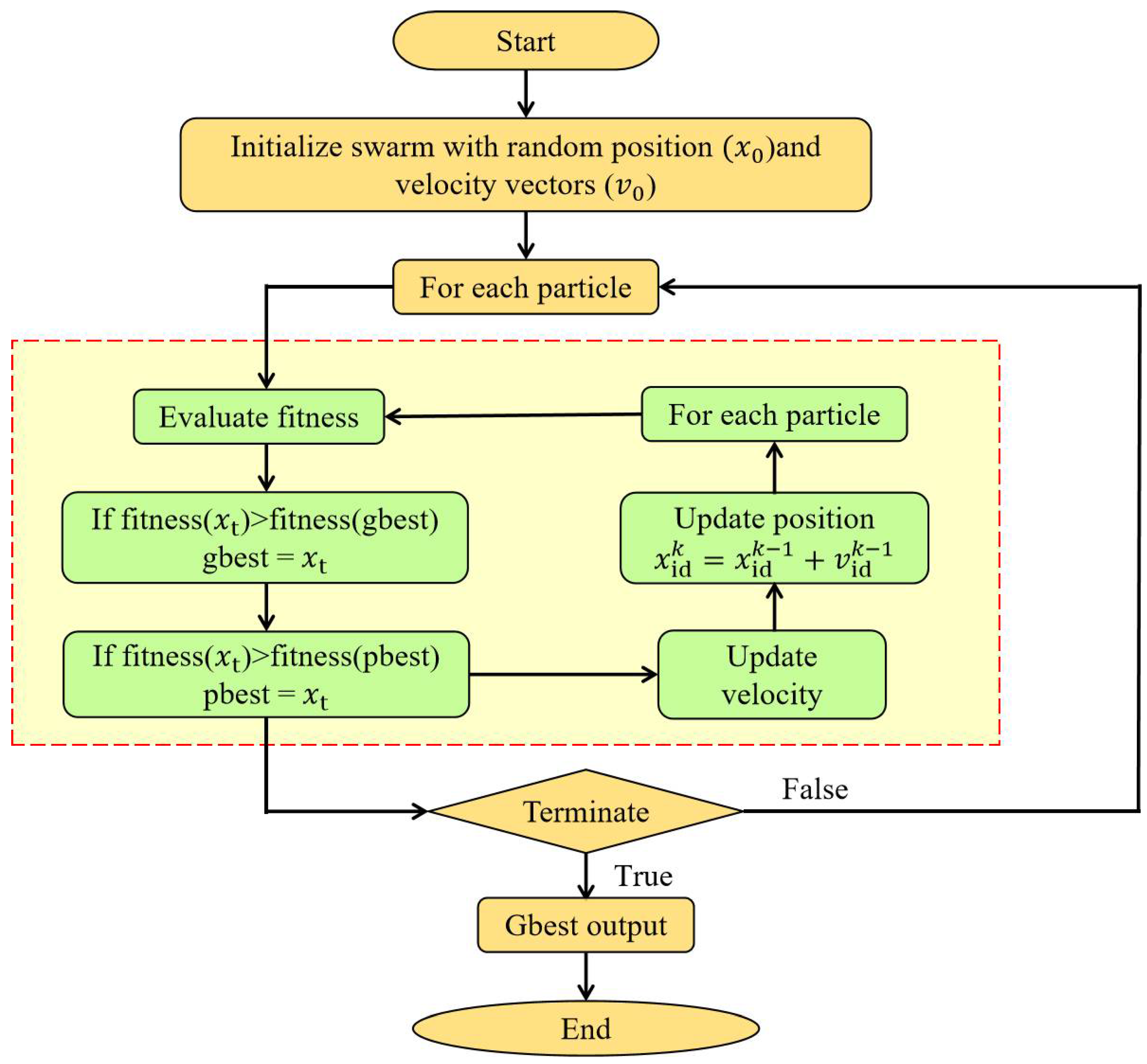
2.2. Particle Swarm Optimization
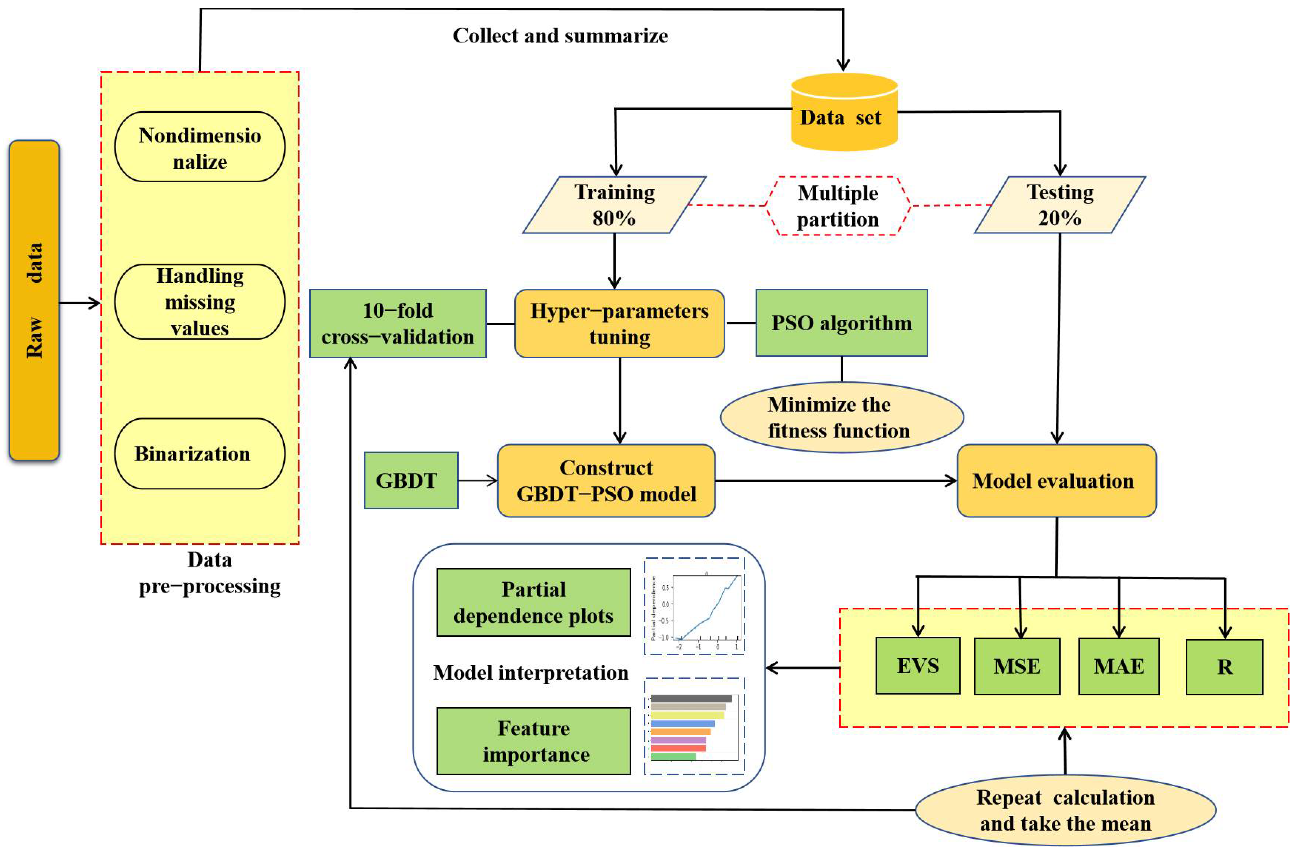
3. Methods
3.1. Established Dataset
3.2. Hyperparameters Tuning
3.3. Evaluation and Interpretation of the Model
4. Results, Discussion, and Concluding Remarks
4.1. Results of the Hyperparameters Tuning
4.2. Results of the Optimum GBDT Model
4.3. Relative Importance of Influencing Variables
4.4. Superiority and Limitations
5. Conclusions
- (1)
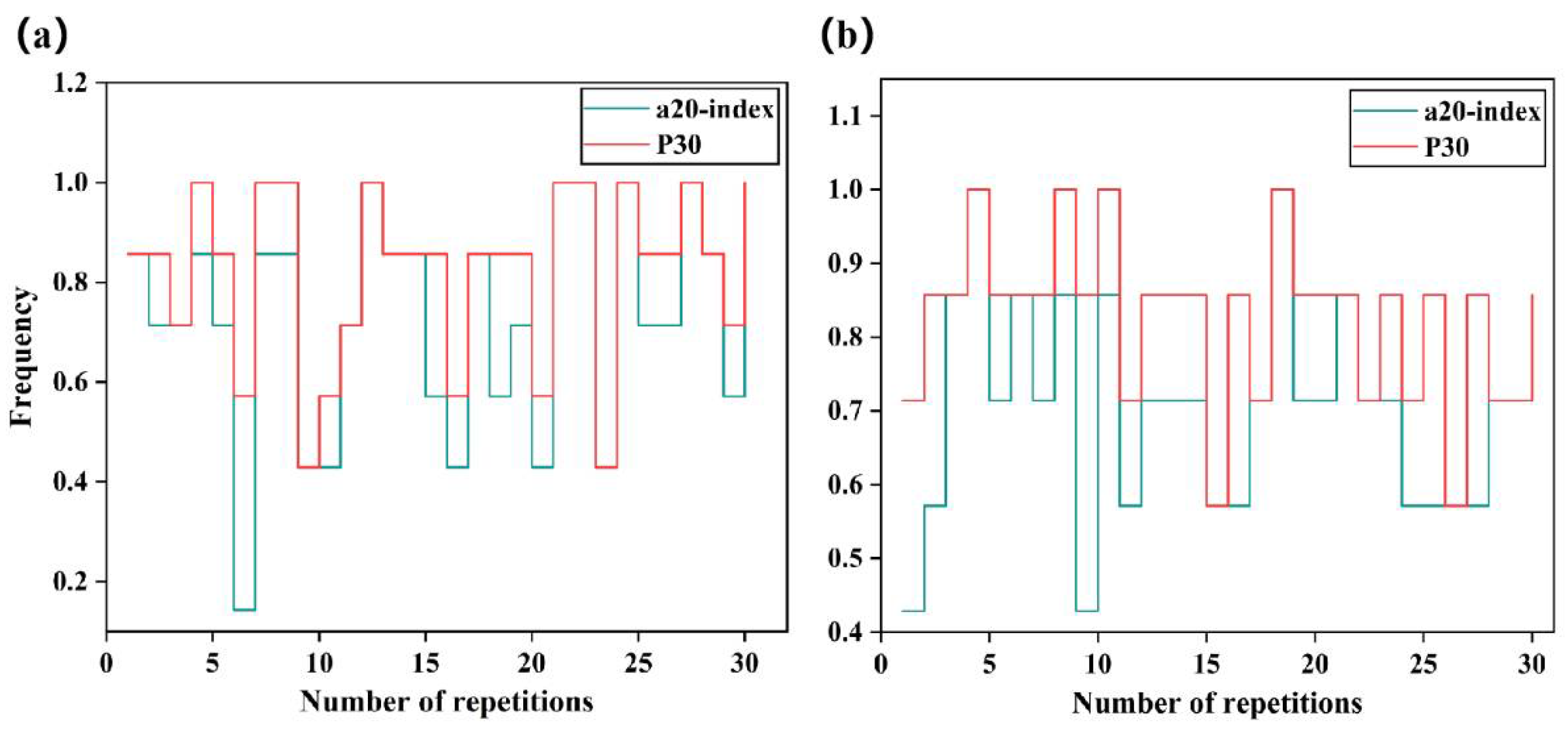
- PSO was efficient in the hyperparameter tuning of GBDT models with maximum R values of 0.987 on the Qu dataset and 0.957 on the up dataset; these results were achieved in the first 10 PSO iterations.
- (2)
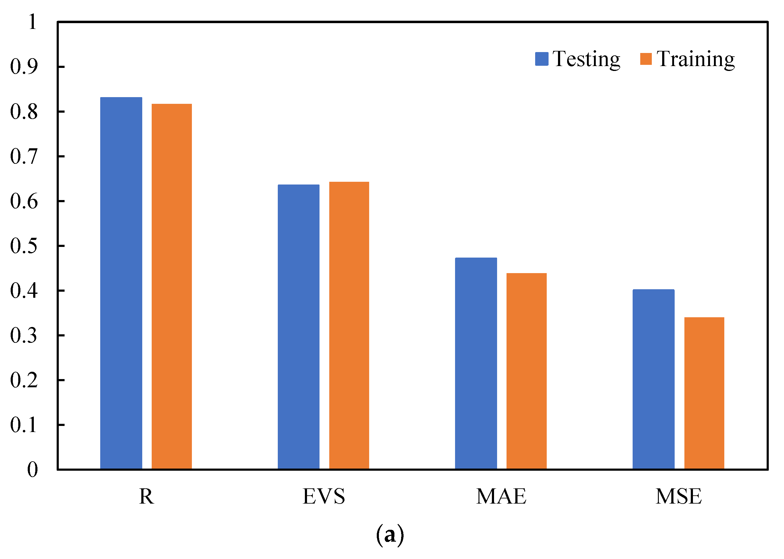
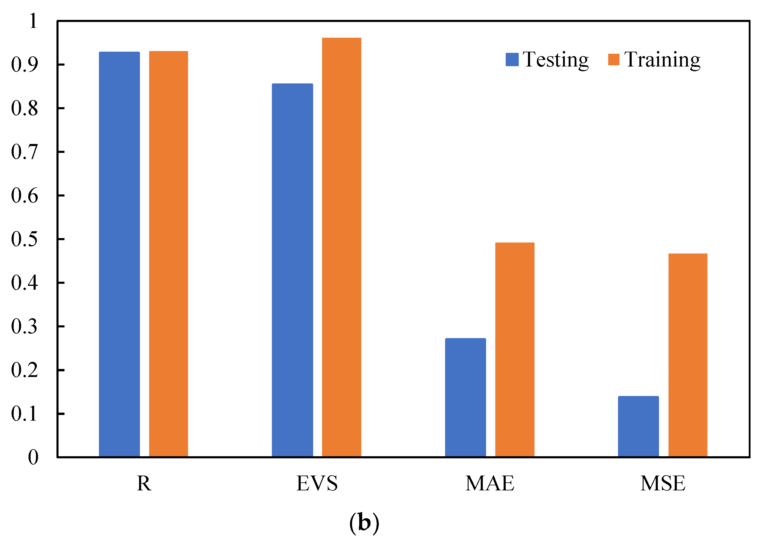
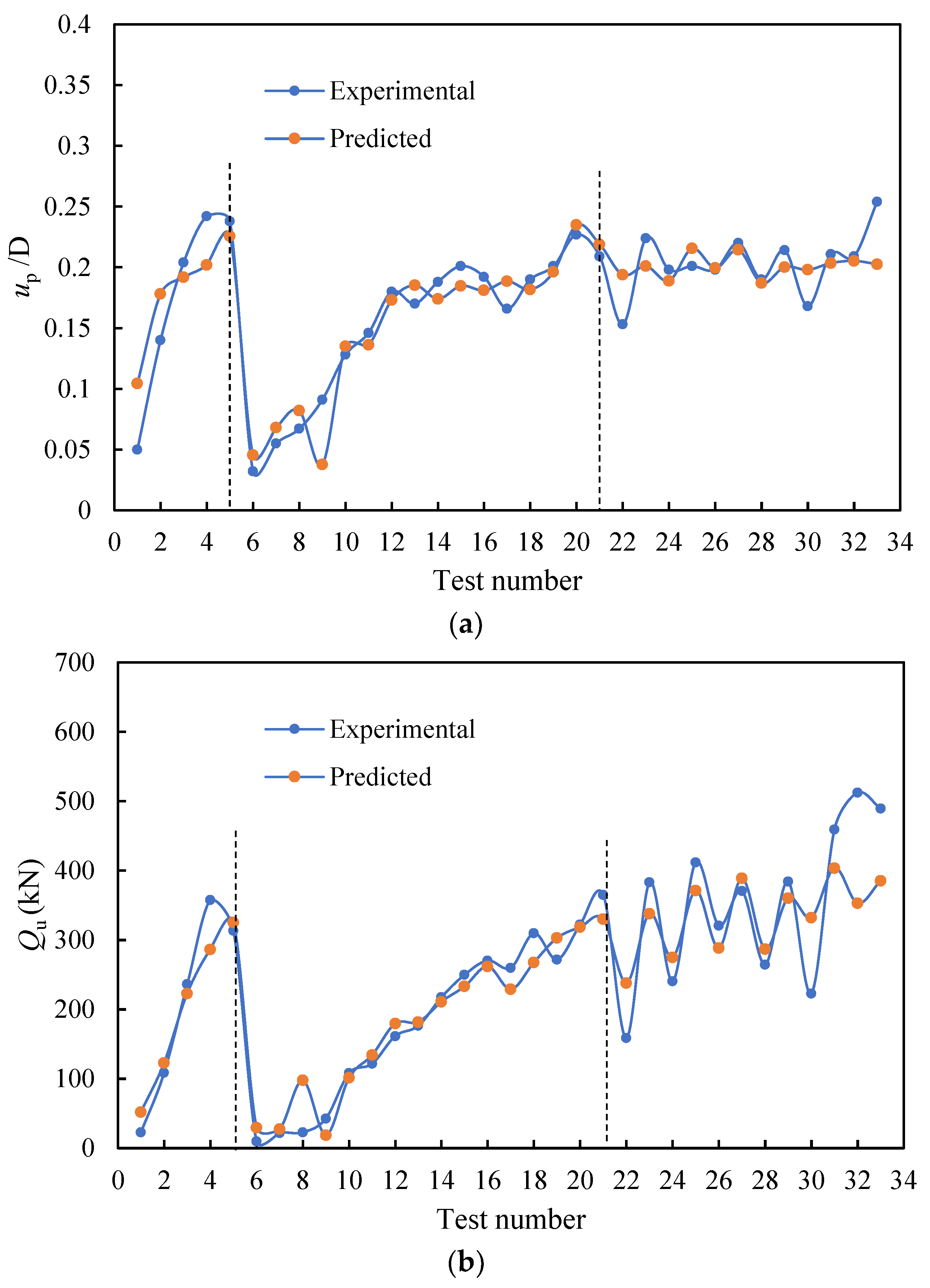
- The optimal GBDT–PSO model has a high generalization ability. For Qu and up, the R values on the testing set were up to 0.93 and 0.82, respectively, and the a20-index values were 0.70 and 0.724, indicating that the model has predictive ability for the lifting behavior of spiral anchors in sand.
- (3)
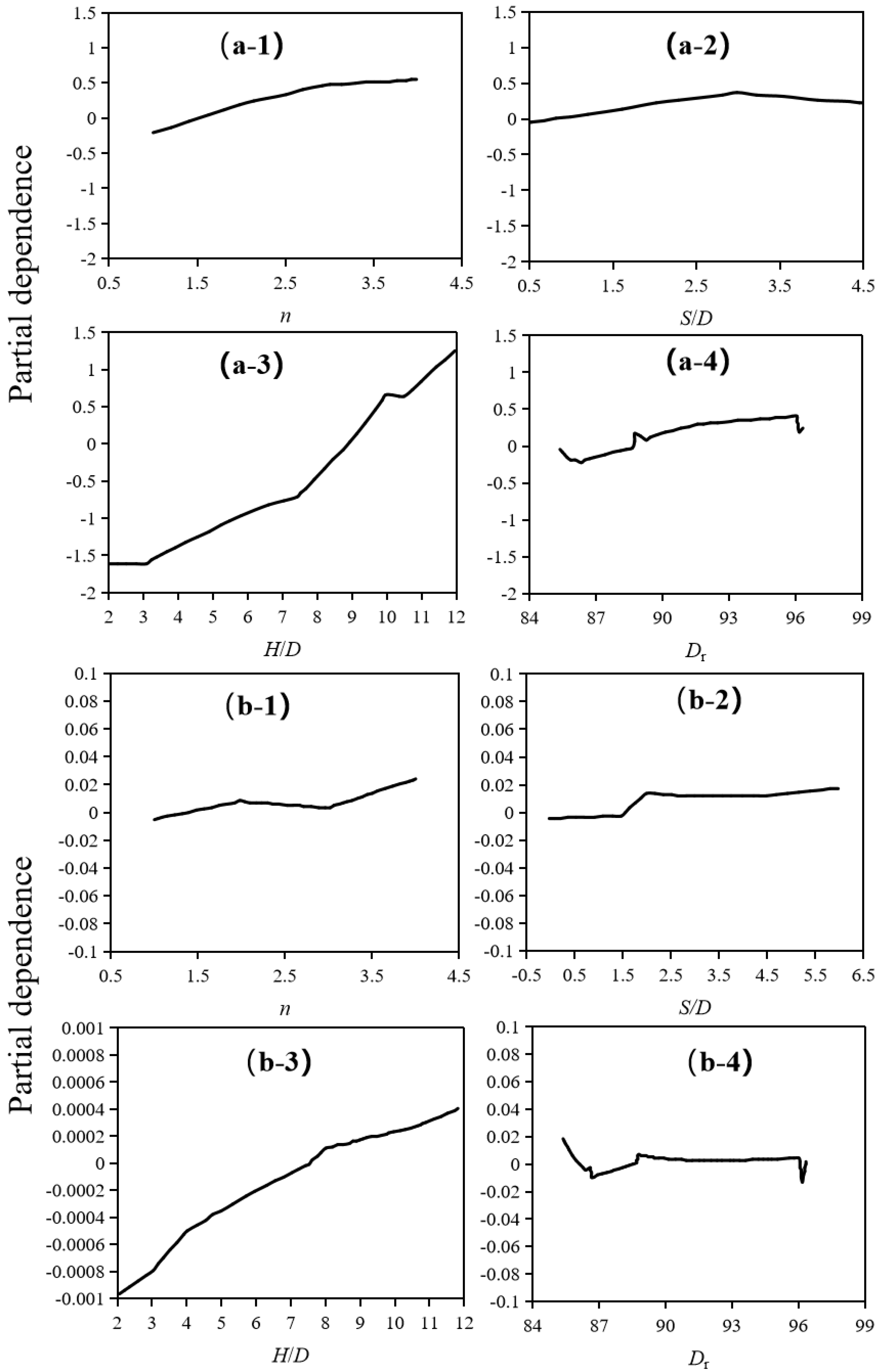
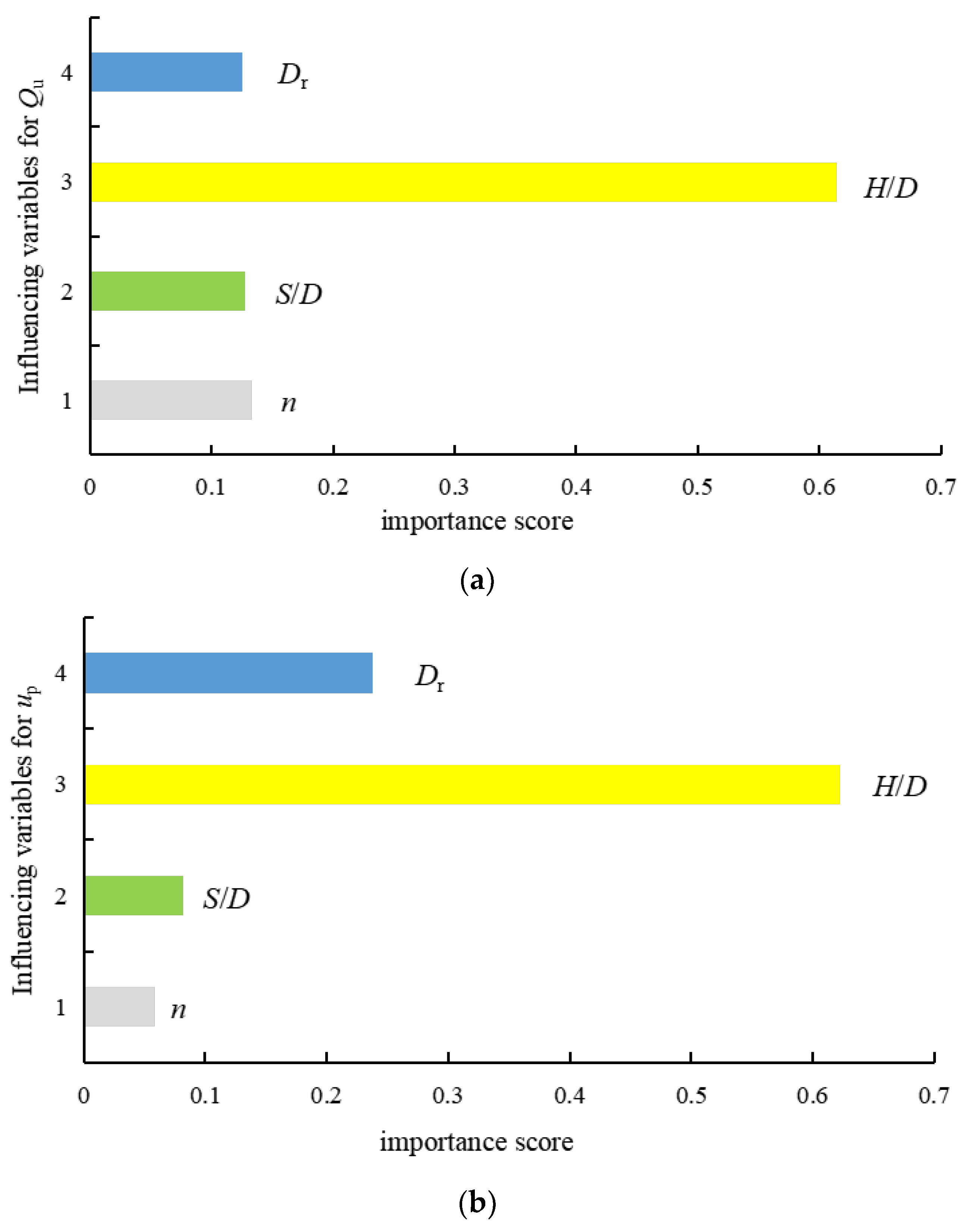
- The embedment ratio, H/D, was found to be the most important variable; however, the helix spacing ratio, S/D, was found to have less influence on the capacity of adjacent helices when S/D > 6. The influence of other input variable is not obvious.
Author Contributions
Funding
Institutional Review Board Statement
Informed Consent Statement
Data Availability Statement
Acknowledgments
Conflicts of Interest
Nomenclature
| Dr | relative density of soil |
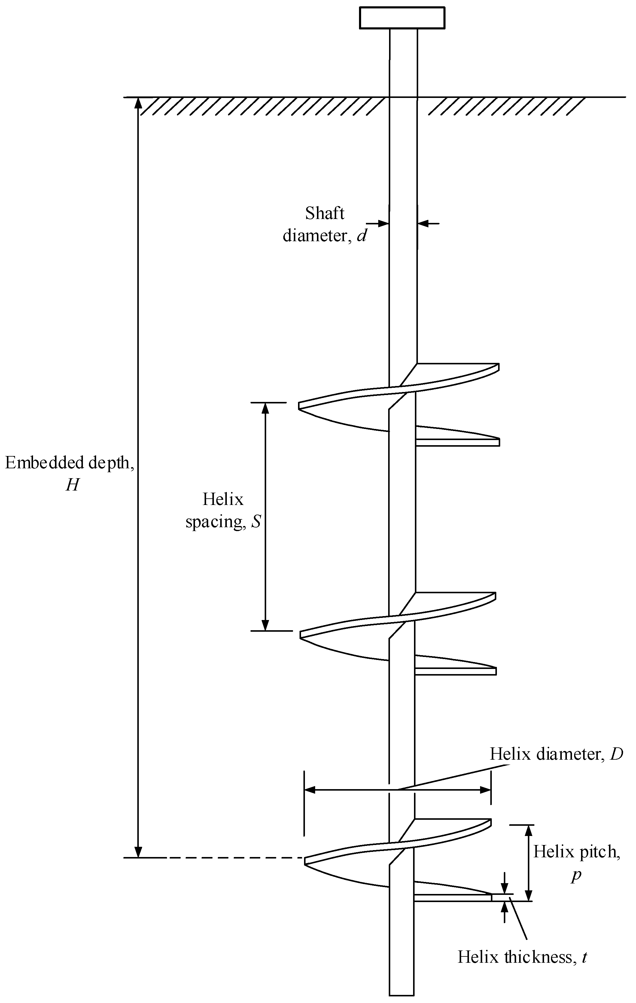
| H | embedment depth of lowest helix |
| D | helix diameter |
| d | shaft diameter |
| S | helix spacing |
| n | number of helices |
| t | thickness of helix |
| p | the pitch of helix |
| up | the anchor mobilization distance |
| Qu | the ultimate monotonic uplift resistance |
| Nγ | the anchor uplift capacity factor |
| γ | the unit weight of sand |
| A | the projected area of a single helix or plate |
| AI | artificial intelligence |
| ANN | artificial neural network |
| GBDT | gradient-boosting decision trees |
| PSO | particle swarm optimization |
| CART | classification and regression tree |
| EVS | explained variance score |
| MSE | mean squared error |
| MAE | mean absolute error |
| R | correlation coefficient |
References
- Lutenegger, A. Behavior of multi-helix screw anchors in sand. In Proceedings of the 2011 Pan-Am CGS Geotechnical Conference, Toronto, ON, Canada, 1–10 October 2011. [Google Scholar]
- Merifield, R.S. Ultimate Uplift Capacity of Multiplate Helical Type Anchors in Clay. J. Geotech. Geoenviron. Eng. 2011, 137, 704–716. [Google Scholar] [CrossRef]
- Kwon, O.; Lee, J.; Kim, G.; Kim, I.; Lee, J. Investigation of pullout load capacity for helical anchors subjected to inclined loading conditions using coupled Eulerian-Lagrangian analyses. Comput. Geotech. 2019, 111, 66–75. [Google Scholar] [CrossRef]
- Tucker, K. Uplift capacity of drilled shafts and driven piles in granular materials. In Foundations for Transmission Line Towers; Geotechnical Special Publication 8; ASCE: New York, NY, USA, 1987; pp. 142–159. [Google Scholar]
- Sutherland, H. Uplift resistance of soils. Geotechnique 1988, 38, 493–516. [Google Scholar] [CrossRef]
- Baker, W.H.; Kondner, R.L. Pullout Load Capacity of a Circular Earth Anchor Buried in Sand. Highw. Res. Rec. 1966, 108, 1–10. [Google Scholar]
- Murray, E.; Geddes, J. Uplift of Anchor Plates in Sand. J. Geotech. Eng. 1987, 113, 202–215. [Google Scholar] [CrossRef]
- Ghaly, A.; Hanna, A.; Hanna, M. Uplift Behavior of Screw Anchors in Sand. I: Dry Sand. J. Geotech. Eng. 1991, 117, 773–793. [Google Scholar] [CrossRef]
- Ghaly, A.; Clemence, S. Pullout Performance of Inclined Helical Screw Anchors in Sand. J. Geotech. Geoenviron. Eng. 1998, 124, 617–627. [Google Scholar] [CrossRef]
- Tagaya, K.; Scott, R.; Aboshi, H. Pullout Resistance of Buried Anchor in Sand. Soils Found. 1988, 28, 114–130. [Google Scholar] [CrossRef]
- Ilamparuthi, K.; Dickin, E.A.; Muthukrisnaiah, K. Experimental investigation of the uplift behaviour of circular plate anchors embedded in sand. Can. Geotech. J. 2002, 39, 648–664. [Google Scholar] [CrossRef]
- Liu, J.; Liu, M.; Zhu, Z. Sand Deformation around an Uplift Plate Anchor. J. Geotech. Geoenviron. Eng. 2012, 138, 728–737. [Google Scholar] [CrossRef]
- Wang, L.; Zhang, P.; Ding, H.; Tian, Y.; Qi, X. The uplift capacity of single-plate helical pile in shallow dense sand including the influence of installation. Mar. Struct. 2020, 71, 102697. [Google Scholar] [CrossRef]
- Ovesen, N.K. Centrifuge tests of the uplift capacity of anchors. In Proceedings of the 10th International Conference on Soil Mechanics and Foundation Engineering, Stockholm, Sweden, 15–19 June 1981; Volume 1, pp. 717–722. [Google Scholar]
- Dickin, E.A. Uplift Behavior of Horizontal Anchor Plates in Sand. J. Geotech. Eng. 1988, 114, 1300–1317. [Google Scholar] [CrossRef]
- Levesque, C.L. Centrifuge Modelling of Helical Anchors in Sand. Ph.D. Thesis, The University of New Brunswick, Saint John, NB, Canada, 2002. [Google Scholar]
- Tsuha, C.H.C.; Aoki, N.; Rault, G.; Thorel, L.; Garnier, J. Evaluation of the efficiencies of helical anchor plates in sand by centrifuge model tests. Can. Geotech. J. 2012, 49, 1102–1114. [Google Scholar] [CrossRef]
- Hao, D.; Wang, D.; O’Loughlin, C.D.; Gaudin, C. Tensile monotonic capacity of helical anchors in sand: Interaction between helices. Can. Geotech. J. 2019, 56, 1534–1543. [Google Scholar] [CrossRef]
- Park, H.; Cho, C. Neural Network Model for Predicting the Resistance of Driven Piles. Mar. Georesour. Geotechnol. 2010, 28, 324–344. [Google Scholar] [CrossRef]
- Momeni, E.; Nazir, R.; Armaghani, D.J.; Maizir, H. Prediction of pile bearing capacity using a hybrid genetic algorithm-based ANN. Measurement 2014, 57, 122–131. [Google Scholar] [CrossRef]
- Baziar, M.H.; Aziakandi, A.S.; Kashkooli, A. Prediction of pile settlement based on cone penetration test results: An ANN approach. KSCE J. Civ. Eng. 2015, 19, 98–106. [Google Scholar] [CrossRef]
- Suman, S.; Das, S.K.; Mohanty, R. Prediction of friction capacity of driven piles in clay using artificial intelligence techniques. Int. J. Geotech. Eng. 2016, 10, 469–475. [Google Scholar] [CrossRef]
- Alzabeebee, S.; Chapman, D.N. Evolutionary computing to determine the skin friction capacity of piles embedded in clay and evaluation of the available analytical methods. Transp. Geotech. 2020, 24, 100372. [Google Scholar] [CrossRef]
- Alzabeebee, S.; Zuhaira, A.A.; Al-Hamd, R.K.S. Development of an optimized model to compute the undrained shaft friction adhesion factor of bored piles. Geomech. Eng. 2022, 28, 397–404. [Google Scholar]
- Goh, A.T.; Kulhawy, F.H.; Chua, C. Bayesian Neural Network Analysis of Undrained Side Resistance of Drilled Shafts. J. Geotech. Geoenviron. Eng. 2005, 131, 84–93. [Google Scholar] [CrossRef]
- Zhang, W.; Goh, A.T. Multivariate adaptive regression splines and neural network models for prediction of pile drivability. Geosci. Front. 2016, 7, 45–52. [Google Scholar] [CrossRef]
- Moayedi, H.; Moatamediyan, A.; Nguyen, H.; Bui, X.-N.; Bui, D.T.; Rashid, A.S.A. Prediction of ultimate bearing capacity through various novel evolutionary and neural network models. Eng. Comput. 2020, 36, 671–687. [Google Scholar] [CrossRef]
- Mosallanezhad, M.; Moayedi, H. Developing hybrid artificial neural network model for predicting uplift resistance of screw piles. Arab. J. Geosci. 2017, 10, 479. [Google Scholar] [CrossRef]
- Javadi, A.; Asr, A.A.; Johari, A.; Faramarzi, A.; Toll, D. Modelling stress–strain and volume change behaviour of unsaturated soils using an evolutionary based data mining technique, an incremental approach. Eng. Appl. Artif. Intell. 2012, 25, 926–933. [Google Scholar] [CrossRef]
- Schiavon, J.; Tsuha, C.; Thorel, L. Scale effect in centrifuge tests of helical anchors in sand. Int. J. Phys. Model. Geotech. 2016, 16, 185–196. [Google Scholar] [CrossRef]
- Elith, J.H.; Graham, C.P.; Anderson, R.; Dudík, M.; Ferrier, S.; Guisan, A.; Hijmans, R.J.; Huettmann, F.; Leathwick, J.R.; Lehmann, A.; et al. Novel methods improve prediction of species’ distributions from occurrence data. Ecography 2006, 29, 129–151. [Google Scholar] [CrossRef]
- Olson, R.S.; Cava, W.L.; Mustahsan, Z.; Varik, A.; Moore, J.H. Data-driven advice for applying machine learning to bioinformatics problems. In Biocomputing 2018; World Scientific: Kohala Coast, HI, USA, 2018; pp. 192–203. [Google Scholar] [CrossRef]
- Zhou, J.; Li, X.; Mitri, H.S. Comparative performance of six supervised learning methods for the development of models of hard rock pillar stability prediction. Nat. Hazards 2015, 79, 291–316. [Google Scholar] [CrossRef]
- Byrne, B.W.; Houlsby, G.T. Helical piles: An innovative foundation design option for offshore wind turbines. Philos. Trans. R. Soc. Lond. Ser. A Math. Phys. Eng. Sci. 2015, 373, 20140081. [Google Scholar] [CrossRef]
- Ren, Q.; Ding, L.; Dai, X.; De Schutter, G. Prediction of Compressive Strength of Concrete with Manufactured Sand by Ensemble Classification and Regression Tree Method. J. Mater. Civ. Eng. 2021, 33, 04021135. [Google Scholar] [CrossRef]
- Tyralis, H.; Papacharalampous, G. Boosting algorithms in energy research: A systematic review. Neural Comput. Appl. 2021, 33, 14101–14117. [Google Scholar] [CrossRef]
- Zou, Y.; Chen, Y.; Deng, H. Gradient Boosting Decision Tree for Lithology Identification with Well Logs: A Case Study of Zhaoxian Gold Deposit, Shandong Peninsula, China. Nonrenew. Resour. 2021, 30, 3197–3217. [Google Scholar] [CrossRef]
- Chou, J.P.E.; Chiu, C.; Farfoura, M.; Al-Taharwa, I. Optimizing the Prediction Accuracy of Concrete Compressive Strength Based on a Comparison of Data-Mining Techniques. J. Comput. Civ. Eng. 2011, 25, 242–253. [Google Scholar] [CrossRef]
- Du, X.; Xu, H.; Zhu, F. A data mining method for structure design with uncertainty in design variables. Comput. Struct. 2020, 244, 106457. [Google Scholar] [CrossRef]
- Kiani, J.; Camp, C.; Pezeshk, S. On the application of machine learning techniques to derive seismic fragility curves. Comput. Struct. 2019, 218, 108–122. [Google Scholar] [CrossRef]
- Carrizosa, E.; Molero-Río, C.; Morales, D.R. Mathematical optimization in classification and regression trees. TOP 2021, 29, 5–33. [Google Scholar] [CrossRef]
- Dimou, C.; Koumousis, V. Reliability-Based Optimal Design of Truss Structures Using Particle Swarm Optimization. J. Comput. Civ. Eng. 2009, 23, 100–109. [Google Scholar] [CrossRef]
- Bai, W.; Wang, Z.; Liu, H.; Yu, D.; Chen, C.; Zhu, M. Optimisation of the finite-difference scheme based on an improved PSO algorithm for elastic modelling. Explor. Geophys. 2020, 52, 419–430. [Google Scholar] [CrossRef]
- Yan, J.; Gao, Y.; Yu, Y.; Xu, H.; Xu, Z. A Prediction Model Based on Deep Belief Network and Least Squares SVR Applied to Cross-Section Water Quality. Water 2020, 12, 1929. [Google Scholar] [CrossRef]
- Jia, B.; Wu, J.; Du, J.; Ji, Y.; Zhu, L. A prediction model for the secure issuance scale of Chinese local government bonds. Kybernetes 2020, 50, 1125–1143. [Google Scholar] [CrossRef]
- Chow, S.H.; O’Loughlin, C.D.; Corti, R.; Gaudin, C.; Diambra, A. Drained cyclic capacity of plate anchors in dense sand: Experimental and theoretical observations. Géotech. Lett. 2015, 5, 80–85. [Google Scholar] [CrossRef]
- Zhu, F.Y.; Bienen, B.; O’Loughlin, C.; Cassidy, M.J.; Morgan, N. Suction caisson foundations for offshore wind energy: Cyclic response in sand and sand over clay. Géotechnique 2019, 69, 924–931. [Google Scholar] [CrossRef]
- Qi, C.; Fourie, A.; Chen, Q.; Zhang, Q. A strength prediction model using artificial intelligence for recycling waste tailings as cemented paste backfill. J. Clean. Prod. 2018, 183, 566–578. [Google Scholar] [CrossRef]
- Khan, M.A.; Zafar, A.; Farooq, F.; Javed, M.F.; Alyousef, R.; Alabduljabbar, H. Geopolymer Concrete Compressive Strength via Artificial Neural Network, Adaptive Neuro Fuzzy Interface System, and Gene Expression Programming With K-Fold Cross Validation. Front. Mater. 2021, 8, 621163. [Google Scholar] [CrossRef]
- Alzabeebee, S.; Alshkane, Y.M.; Al-Taie, A.J.; Rashed, K.A. Soft computing of the recompression index of fine-grained soils. Soft Comput. 2021, 25, 15297–15312. [Google Scholar] [CrossRef]
- Alzabeebee, S.; Alshkane, Y.M.; Rashed, K.A. Evolutionary computing of the compression index of fine-grained soils. Arab. J. Geosci. 2021, 14, 2040. [Google Scholar] [CrossRef]
- Alzabeebee, S.; Mohammed, D.A.; Alshkane, Y.M. Experimental Study and Soft Computing Modeling of the Unconfined Compressive Strength of Limestone Rocks Considering Dry and Saturation Conditions. Rock Mech. Rock Eng. 2022, 55, 5535–5554. [Google Scholar] [CrossRef]
- Alzabeebee, S. Explicit soft computing model to predict the undrained bearing capacity of footing resting on aggregate pier reinforced cohesive ground. Innov. Infrastruct. Solut. 2022, 7, 105. [Google Scholar] [CrossRef]
- Zhang, L.; Wu, X.; Ji, W.; AbouRizk, S.M. Intelligent Approach to Estimation of Tunnel-Induced Ground Settlement Using Wavelet Packet and Support Vector Machines. J. Comput. Civ. Eng. 2017, 31, 04016053. [Google Scholar] [CrossRef]
- Jin, X.; Zhu, X.; Li, S.; Wang, W.; Qi, H. Predicting soil available phosphorus by hyperspectral regression method based on gradient boosting decision tree. Laser Optoelectron. Prog. 2019, 56, 131102. [Google Scholar] [CrossRef]
- Ye, Y.; Xiong, Y.; Zhou, Q.; Wu, J.; Li, X.; Xiao, X. Comparison of machine learning methods and conventional logistic regressions for predicting gestational diabetes using routine clinical data: A retrospective cohort study. J. Diabetes Res. 2020, 2020, 4168340. [Google Scholar] [CrossRef] [PubMed]
- Jun, M.-J. A comparison of a gradient boosting decision tree, random forests, and artificial neural networks to model urban land use changes: The case of the Seoul metropolitan area. Int. J. Geogr. Inf. Sci. 2021, 35, 2149–2167. [Google Scholar] [CrossRef]
- Breiman, L.; Friedman, J.; Olshen, R.; Stone, C.J. Classification and Regression Trees, Wadsworth Statistics; Probability Series; Wadsworth: Belmont, CA, USA, 1984. [Google Scholar] [CrossRef]
- Friedman, J.H. Greedy function approximation: A gradient boosting machine. Ann. Stat. 2001, 29, 1189–1232. [Google Scholar] [CrossRef]
- Giampa, J.; Bradshaw, A.; Schneider, J. Influence of Dilation Angle on Drained Shallow Circular Anchor Uplift Capacity. Int. J. Géoméch. 2017, 17, 04016056. [Google Scholar] [CrossRef]
- Wang, J.; Haigh, S.K.; Forrest, G.; Thusyanthan, N.I. Mobilization Distance for Upheaval Buckling of Shallowly Buried Pipelines. J. Pipeline Syst. Eng. Pract. 2012, 3, 106–114. [Google Scholar] [CrossRef]


| Helical Anchor | Soil | ||
|---|---|---|---|
| Dimensions | Value | Properties | Value |
| Helix diameter, D (mm) | 20 | Specific gravity, Gs | 2.65 |
| Helix pitch, p (mm) | 5 | Median grain size, d50 (mm) | 0.25 |
| Helix thickness, t (mm) | 2 | Coefficient of uniformity, Cu | 1.87 |
| Shaft diameter, d (mm) | 4.7 | Coefficient of curvature, Cc | 0.938 |
| Number of helix, n | 0, 1, 2, 3, 4 | Maximum void ratio, emax | 0.703 |
| Helix spacing, S | 1.5, 2, 3, 4.5, 6 D | Minimum void ratio, emin | 0.516 |
| Critical state friction angle, | 31 | ||
| Experiment Number | N | S/D | H/D | Dr (%) | up /D | Qu (kN) |
|---|---|---|---|---|---|---|
| T1 | 1 | 0 | 3 | 85.8 | 0.050 | 22.9 |
| T2 | 1 | 0 | 6 | 85.8 | 0.140 | 108.7 |
| T3 | 1 | 0 | 9 | 85.8 | 0.204 | 236.2 |
| T4 | 1 | 0 | 12 | 85.8 | 0.242 | 357.5 |
| T5 | 1 | 0 | 85.4 | 0.238 | 313.4 | |
| T6 | 1 | 0 | 2 | 86.7 | 0.032 | 9.9 |
| T7 | 1 | 0 | 3 | 86.4 | 0.055 | 22.1 |
| T8 | 1 | 0 | 96.2 | 0.067 | 22.9 | |
| T9 | 1 | 0 | 4 | 86.7 | 0.091 | 42.9 |
| T10 | 1 | 0 | 6 | 86.4 | 0.128 | 108.1 |
| T11 | 1 | 0 | 96.2 | 0.146 | 121.7 | |
| T12 | 1 | 0 | 7.5 | 90.0 | 0.180 | 161.6 |
| T13 | 1 | 0 | 8 | 86.4 | 0.170 | 176.4 |
| T14 | 1 | 0 | 96.4 | 0.188 | 217.6 | |
| T15 | 1 | 0 | 9 | 88.8 | 0.201 | 249.9 |
| T16 | 1 | 0 | 96.1 | 0.192 | 270.3 | |
| T17 | 1 | 0 | 96.2 | 0.166 | 260.0 | |
| T18 | 1 | 0 | 10 | 96.4 | 0.190 | 309.6 |
| T19 | 1 | 0 | 10.5 | 90.0 | 0.201 | 271.8 |
| T20 | 1 | 0 | 12 | 85.4 | 0.227 | 322.1 |
| T21 | 1 | 0 | 91.7 | 0.209 | 364.9 | |
| T22 | 2 | 1.5 | 7.5 | 88.7 | 0.153 | 158.8 |
| T23 | 2 | 1.5 | 12 | 86.6 | 0.224 | 383.1 |
| T24 | 2 | 3 | 9 | 89.3 | 0.198 | 240.7 |
| T25 | 2 | 3 | 12 | 86.7 | 0.201 | 412.0 |
| T26 | 2 | 4.5 | 10.5 | 89.3 | 0.198 | 320.9 |
| T27 | 2 | 4.5 | 12 | 86.6 | 0.220 | 370.7 |
| T28 | 2 | 6 | 9 | 96.2 | 0.190 | 264.7 |
| T29 | 2 | 6 | 12 | 86.7 | 0.214 | 384.2 |
| T30 | 3 | 1.5 | 9 | 89.3 | 0.168 | 222.9 |
| T31 | 3 | 3 | 12 | 88.8 | 0.211 | 459.5 |
| T32 | 3 | 1.5 | 12 | 96.1 | 0.209 | 512.6 |
| T33 | 4 | 2 | 12 | 90.0 | 0.254 | 489.4 |
| Variables | Type | Standard Deviation | Maximum | Minimum | Mean | Kurtosis | Skewness |
|---|---|---|---|---|---|---|---|
| N | Input | 0.783 | 4.000 | 1.000 | 1.515 | 1.844 | 1.464 |
| S/D | Input | 1.815 | 6.000 | 0.000 | 1.152 | 1.363 | 1.473 |
| H/D | Input | 3.107 | 12.000 | 2.000 | 8.788 | −0.490 | −0.705 |
| Dr | Input | 3.992 | 96.400 | 85.400 | 89.724 | −0.959 | 0.737 |
| up/D | Output | 0.057 | 0.254 | 0.032 | 0.174 | 0.652 | −1.129 |
| Qu | Output | 137.747 | 512.600 | 9.900 | 248.182 | −0.720 | −0.098 |
| Hyperparameters | Explanation | Type | Tuning Range |
|---|---|---|---|
| Max_depth | The maximum depth of the CART | Integer | 3–15 |
| Min_samples_split | The minimum number of samples required to split an internal node | Integer | 2–15 |
| Min_samples_leaf | The minimum number of samples at the leaf node | Integer | 1–15 |
| Max_RT | The maximum number of CART models in GBDT | Integer | 50–2000 |
| Learning rate | The learning rate shrinks the contribution of each CART model | Float | 0.01–1 |
| Max_features | The number of features to consider during tree splitting | Float | 0.4–1 |
| Hyperparameters | Qu Dataset | up Dataset |
|---|---|---|
| Max_depth | 4 | 15 |
| Min_samples_split | 7 | 7 |
| Min_samples_leaf | 1 | 1 |
| Max_RT | 1319 | 873 |
| Learning rate | 0.061 | 0.890 |
| Max_features | 1 | 1 |
Publisher’s Note: MDPI stays neutral with regard to jurisdictional claims in published maps and institutional affiliations. |
© 2022 by the authors. Licensee MDPI, Basel, Switzerland. This article is an open access article distributed under the terms and conditions of the Creative Commons Attribution (CC BY) license (https://creativecommons.org/licenses/by/4.0/).
Share and Cite
Wang, L.; Wu, M.; Chen, H.; Hao, D.; Tian, Y.; Qi, C. Efficient Machine Learning Models for the Uplift Behavior of Helical Anchors in Dense Sand for Wind Energy Harvesting. Appl. Sci. 2022, 12, 10397. https://doi.org/10.3390/app122010397
Wang L, Wu M, Chen H, Hao D, Tian Y, Qi C. Efficient Machine Learning Models for the Uplift Behavior of Helical Anchors in Dense Sand for Wind Energy Harvesting. Applied Sciences. 2022; 12(20):10397. https://doi.org/10.3390/app122010397
Chicago/Turabian StyleWang, Le, Mengting Wu, Hongzhen Chen, Dongxue Hao, Yinghui Tian, and Chongchong Qi. 2022. "Efficient Machine Learning Models for the Uplift Behavior of Helical Anchors in Dense Sand for Wind Energy Harvesting" Applied Sciences 12, no. 20: 10397. https://doi.org/10.3390/app122010397
APA StyleWang, L., Wu, M., Chen, H., Hao, D., Tian, Y., & Qi, C. (2022). Efficient Machine Learning Models for the Uplift Behavior of Helical Anchors in Dense Sand for Wind Energy Harvesting. Applied Sciences, 12(20), 10397. https://doi.org/10.3390/app122010397