1. Introduction
Metaheuristics for combinatorial optimisation problems [
1] are usually inspired by natural processes, such as Darwin’s theory of evolution, with evolutionary algorithms (EA) being a classic example [
2]. Specifically, bio-inspired algorithms such as genetic algorithms (GA) [
3,
4], simulated annealing (SA) [
5], particle swarm optimisation (PSO) [
6], and ant colony optimisation (ACO) [
7], are able to find good (usually optimum) solutions to highly complex real-world problems in reasonable computing times. They start with a set of initial candidate solutions and iteratively generate new ones in a chain of increasingly fitted populations toward the optimum of the problem. They are non-deterministically guided and use intelligent search balances in the exploration of the search space. They exploit its more promising regions to hopefully find the optimal solution to the problem being solved.
One real-world problem, which has features that are difficult to solve by using exact techniques, is the parameterisation of a swarm of autonomous robots to efficiently arrange in a formation. Reported applications of robot formation found in the literature comprise surveillance [
8], synchronisation of spacecraft [
9], autonomous navigation [
10], load transportation in precision agriculture [
11], urban search and rescue [
12], and marine applications [
13], etc. They require different control schemas, e.g., whether they need a collision-avoidance strategy, making it difficult to find an architecture that suits all the requirements. Moreover, problems related to robot-formation systems usually present unknown initial positions of the swarm members, as well as the need for path planning from these positions to the final locations. Systems having predefined final positions also present challenging adaptability to real situations, especially when the initial positions are not always known in advance or there are robot failures.
Our formation proposal consists of a range- and bearing-based approach in which the unmanned aerial vehicles (UAVs) in the swarm self-organise to arrange a final desired formation, surrounding an object such as a rogue drone in a sphere-like shape. It is part of a swarm-based counter UAS (C-UAS) system. We do not use a global coordinate system nor a different, intelligent node in the swarm. We just let the UAVs make their own local decisions based on local information. There is an exclusion zone (sphere) around the central point of the formation to avoid collisions with the rogue drone while the formation algorithm itself avoids collisions between the swarm members. Other applications can be derived from our proposal, such as asteroid observation, provided that the number of robots (probes) is high enough and the desired formation radius is achievable. Our proposal is tested on three case studies comprising swarms of three, five, and 10 UAVs. We proposed four individual UAV parameters and designed a hybrid EA to optimise them in order to achieve proper formations in all the 300 scenarios studied. The main contributions of this paper are as follows.
A distributed robot 3D formation system able to surround and escort an object of interest is given.
A hybrid EA to optimise the parameters of the formation system providing efficiency and robustness is given.
A study of the EA parameters and an analysis of the proposed genetic operators is presented.
A simulation approach using a multi-physics robot simulator to evaluate the different configurations calculated by the EA is given.
The rest of this paper is organised as follows. In the next section, we review the state of the art related to our proposal. In
Section 3 our robot-formation system is presented. The optimisation approach is discussed in
Section 4, wherein the optimisation algorithm and its parameterisation is described. The experimental results are in
Section 5 and finally,
Section 6 gives our conclusions and future work.
2. Related Works
In this section, we review some research works related to robot formations, including distributed/decentralised approaches [
14] wherein robots self-organise [
15] by using limited local information.
First, we discuss some formation-control articles starting with a distributed method for formation control, as described in [
16]. This article discusses a swarm of aerial robots which self-coordinates by sharing information and obtaining a consensus to navigate throughout a dynamic environment by using a restricted communication and vision range. The authors proposed a motion-planning algorithm based on calculating the convex hull of the robots’ positions and achieving the optimal formation while avoiding obstacles. Their results have been obtained by using four real quad-rotors and Monte Carlo simulation experiments. In our proposal, we obtain different robot formations because our robots are located in a 3D shape inscribed into a sphere, using swarms of up to ten robots. Finally, our formations are achieved by using attracting and repelling forces optimised by an EA.
A non-uniform vector field method is proposed to achieve formations of fixed-wing UAVs in [
17]. The authors use a leader–follower approach and compare their results with a wind-absence method and another one based on unicycle dynamics. The system stability is analysed by using Lyapunov stability theory. Several validations are carried out by comparing simulations by using Gazebo and hardware-in-the-loop experiments using two UAVs. Our approach is different as it does not rely on a leader (all swarm members are in the same hierarchy level). We propose the optimisation of the swarm’s parameters, and simulate up to 10 robots by using the full UAV dynamics.
Secondly, we include some articles in which metaheuristics are used to optimise the robots’ trajectories. In [
18], the authors propose an alternative method by which to achieve distance-based formation by using a GA. It is composed of two phases: formation and obstacle avoidance. Each phase uses a different chromosome. The first codifies the distance and moving angle of each robot to achieve the formation, whereas the second defines the robots’ speed to avoid collisions. The algorithm is tested by using simulations and real robots in experiments in a 2D environment. Although our formation system is also based on distance and angles, we calculate different robot parameters to foster self-organisation by using an EA.
A cooperative method is proposed in [
19] by using a GA and a cellular automata. A team of three robots moves throughout a pre-specified formation pattern by a discretised environment. One of the robots (master) coordinates the rest (slaves) when moving in the desired pattern. A set of robot parameters are calculated by using a GA through simulations to maximise the time in formation and team progress, while minimizing the number of rotations performed by robots. As mentioned before, we propose a different set of parameters focused on the robot collaboration while surrounding a rogue drone in a 3D environment.
Summing up, in our proposal we obtain the UAV formation by using attracting and repelling forces parametrised and optimised by an EA. We use a multi-physics robot simulator to test our proposal on 90 unseen scenarios per case study featuring different initial conditions. We have given some initial steps [
20] in a 2D environment toward the present article in which we have increased the complexity of the formation, proposed and parameterised a hybrid evolutionary algorithm where each robot parameter is optimised individually. To the best of our knowledge, this study involving the optimisation of the swarm parameters for achieving robust 3D formations by using an evolutionary technique followed by the validation by using the ARGoS simulator has not been addressed before.
3. Distributed Formation Algorithm3 (DFA3)
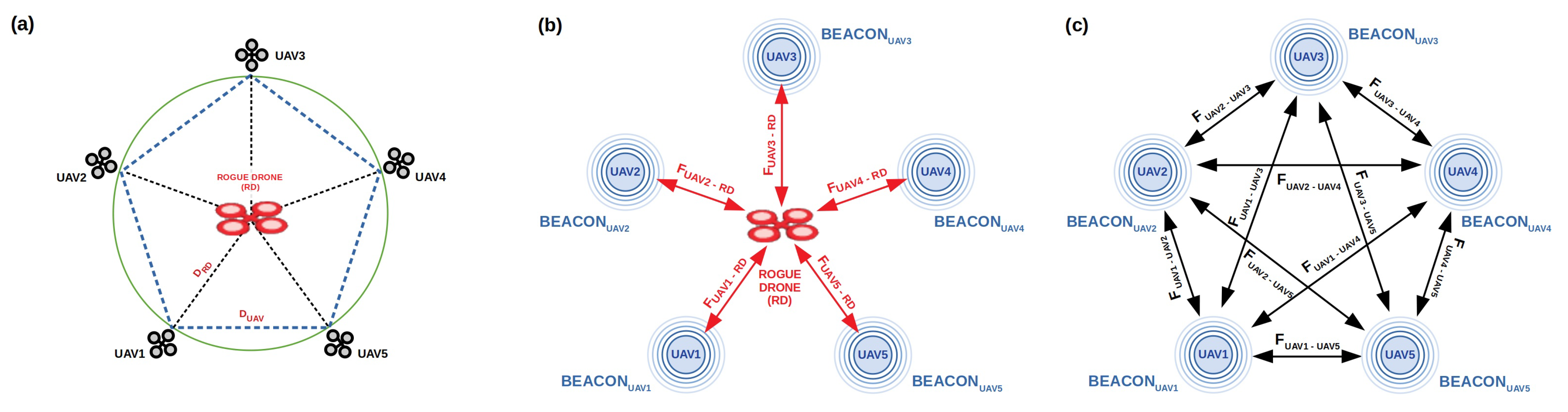
The proposed 3D formation system is focused on a swarm of autonomous flying robots (UAVs), surrounding and escorting a rogue drone out of a restricted area, e.g., an airport, while they conserve a predefined desired distance to the formation centre (
Figure 1a). This is a challenging real-world problem, as achieving stable robot formation systems involves addressing different constraints, such as limited communication range, absence of absolute positions, and uncertain initial conditions.
Each UAV in the swarm receives a beacon signal emitted by each of the other UAVs in the swarm and uses it to calculate its relative orientation and distance to the rest of the UAVs. Given the simplicity of the communications, no protocol is necessary, nor was it implemented. Moreover, no localisation system, such as GPS, is used by the UAVs. Additionally, the UAVs do not have a predefined final position in the formation. The rogue drone is tracked by using its own radio signal in our experiments, although other methods can be used, such as images from cameras, LIDAR data, etc.
The 3D formation is collaboratively built by the UAVs arriving to the area from different positions. They use a series of attracting and repelling forces calculated from the received beacons, to find their final position in the surface of a virtual sphere around the rogue drone. Depending on the number of UAVs, the final shape would be more or less effective as a dissuasive measure. The swarm members are spread by such a virtual sphere to improve their distribution, avoiding being too close each other. Hence, having a reduced number of UAVs could leave too much open space from where the rogue drone might escape. Two types of forces are considered: (i) between each UAV and the rogue drone and (ii) between the UAVs in the swarm (
Figure 1b,c).
The formation problem is defined by
where the distance graph is given by
where
represents the UAVs in the swarm,
represents the edges of the graph indicating the swarm connectivity, and
represents the distances between UAVs (
). Furthermore,
stands for the rogue drone, the distances between the UAVs and the rogue drone are given by
and the problem’s constraints are given by
where
is the desired distance to the rogue drone (formation radius).
We propose four parameters for the swarm members in order to achieve stable formations: a distance threshold to control the attracting/repelling movement between UAVs, the minimum distance to the rogue drone, the intensity of the attracting/repelling force , with respect to the rogue drone, and the moving speed of the UAVs.
The pseudocode of our distributed formation algorithm3 (DFA3) is detailed in Algorithm 1. Each UAV executes the same algorithm with its own parameters, and the same predefined formation radius, i.e., the desired distance to the rogue drone , which is a constant value.
The DFA
3 first initialises the vector
r where the calculation of the resulting attracting/repelling force to/from the rogue drone plus the other UAVs will be stored. Then, for each beacon received, the range and the vertical and horizontal bearings from the other robots are obtained and used to calculate the three components of
r, according to the given distance threshold
. After that, the same calculation is performed with respect to the rogue drone. In this case, depending on the distance from the UAV to the rogue drone and the value of
, an extra intensity
can be applied as a repelling force (
) with respect to the rogue drone. Finally, having calculated the 3D components of
r, the inclination
and azimuth
are calculated as the new moving direction (in 3D space) to be returned to the UAV’s controller.
Figure 2 shows a flow chart of the DFA
3 depicting the beacons being received by the RADIO module to be processed in order to calculate the vector
r by using the optimised parameter set. Finally, the inclination
, azimuth
, and
are sent to the UAV to modify its moving direction.
| Algorithm 1 Distributed formation algorithm3 (DFA3). |
function DFA3() for do ▹ From the other UAVs ▹ Force end for ▹Rogue drone if then ▹ Force intensity end if ▹ Next moving direction (angles) return ▹ Inclination and azimuth end function
|
Table 1 shows the parameters of UAVs running DFA
3. It can be seen that the range of the first three parameters depends on the desired distance
, whereas the robots’ speed is in a fixed range. All these parameter constraints were experimentally calculated.
In the following sections, we describe the optimisation approach including the problem representation, the proposed optimisation algorithm and operators, and its parameterisation. After that, a random search algorithm is proposed as a sanity check, followed by the description of our case studies and our experimental results.
4. Optimisation Approach
As mentioned above, each UAV is configured by using four parameters. Thus, the complete system configuration is represented by the following status vector:
where
is the distance threshold,
is the minimum distance to the rogue drone,
is the attracting/repelling force, and
is the speed, all for each UAV
i in the swarm. Hence, the length of the status vector will depend on the number of UAVs in the swarm (
N).
The proposed evaluation function for this formation problem is shown in Equation (
6). Three terms are added and then averaged for the
M evaluated scenarios (different initial conditions). In doing so, we expect to obtain a more robust solution as the optimisation algorithm will be converging to more general solutions instead of a particular one. The three terms in
are the minimum error (
) and maximum error (
) distance of any UAV in the swarm to the rogue drone, with respect to the desired distance
, and an extra term (
) to foster the UAVs to be spread throughout the surface (sphere) instead of forming local clusters. Because we wish to minimise these terms, the lower the value of
the better:
Having defined the solution vector (problem representation) and the evaluation function, it can be seen that this is a difficult problem to optimise (solve) by an exact method, especially if we take into account its high dimensionality. Hence, in the next section we describe the proposed optimisation technique, a hybrid evolutionary algorithm.
4.1. Evolutionary Algorithm (EA)
The proposed optimisation algorithm is a hybrid EA consisting of two stages (Algorithm 2). First, a genetic algorithm (GA) approach is used during the first 90% of evaluations where the solution space is explored while the GA is converging to competitive solutions [
4]. Secondly, a local search (LS) is applied to the best solution found by the GA in order to explore its neighbourhood. In doing so, this high-level relay hybridisation (HRH) approach [
21] improves the final solution found by the EA.
The GA approach mimics processes present in evolution such as natural selection, gene recombination after reproduction, gene mutation, and the dominance of the fittest individuals over the weaker ones. This is a steady-state GA whereby an offspring of individuals is obtained from the population , so that the auxiliary population Q contains the subset of individuals (10 in our implementation) from the population (20 individuals). This decision finds its justification in the long evaluation times required to evaluate each individual through realistic simulations, especially in the most dense scenarios.
Following the EA’s pseudocode, after initialising
t,
, and
, the initial population
is filled with random individuals by the
Initialisation function. Then, the main loop is executed while the termination condition is not fulfilled (270 evaluations in our case). Binary tournament [
22] was used as selection operator, integer polynomial mutation [
23] as mutation operator, and an elitist replacement was used to update the algorithm population after each generation. Regarding the crossover operator, we propose two candidates: the well-known uniform crossover [
24] and a novel variant adapted to this problem, the drone crossover, both described later in
Section 4.2.
The parameters of the GA were calculated as described in
Section 4.5, using the irace package. After the GA stage, the best solution obtained is fed into the LS performed by the hill climbing algorithm [
25] (HC), which will explore the best solution neighbourhood during the last 30 evaluations. By doing so, we have first explored the search space and then exploited the best solution found.
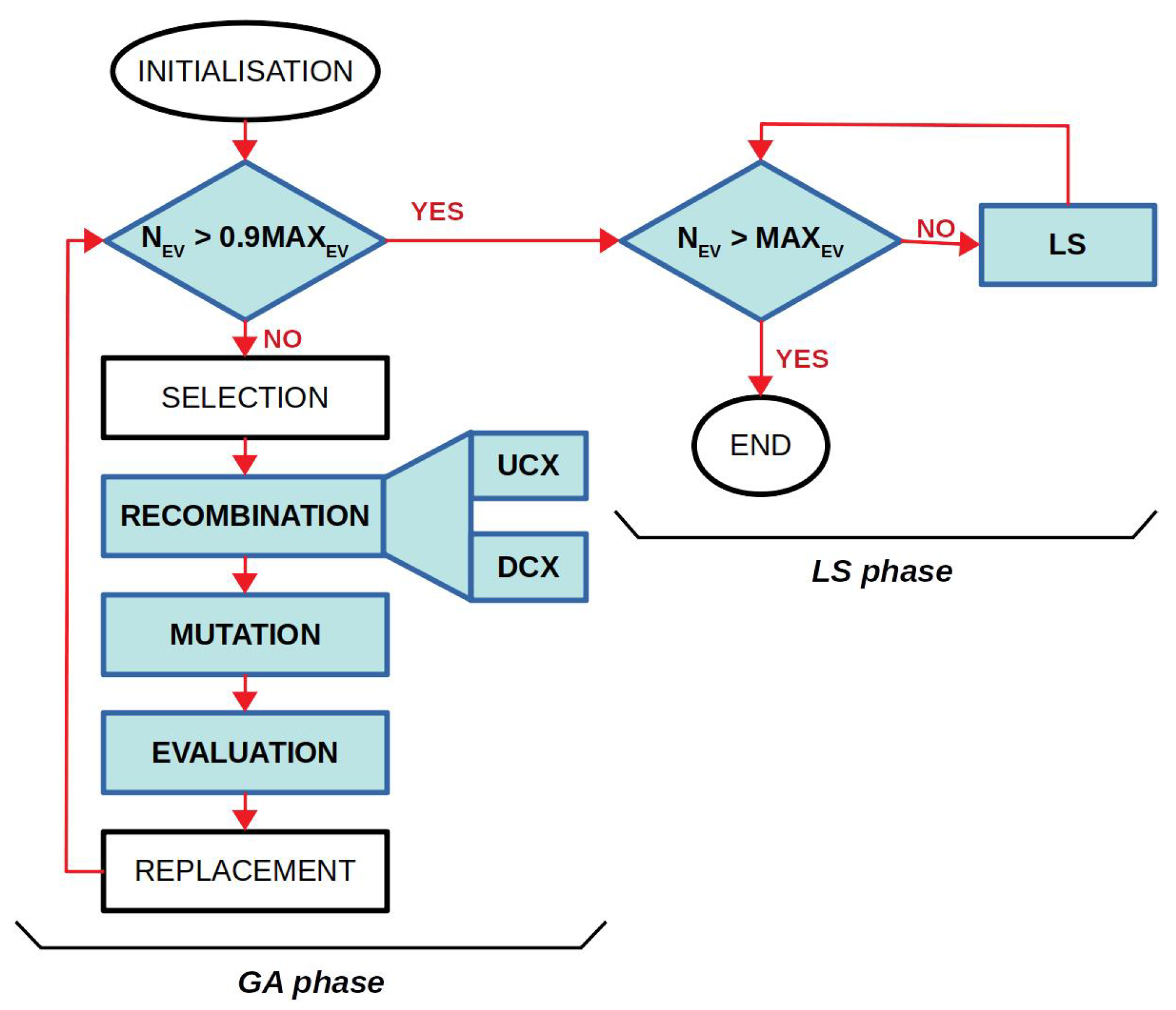
Figure 3 shows the block diagram of the proposed EA where the differences between it and a canonical GA are highlighted by coloured blocks. Specifically, it can be seen that the last 10% of evaluations are used for LS and that in the GA phase, two different recombination operators (crossover) have been proposed to work in combination with a different mutation operator for integer numbers (instead of bit flip).
| Algorithm 2 Pseudocode of the hybrid evolutionary algorithm (EA). |
function EA() ▹ Genetic Algorithm ▹ Q=auxiliary population ▹ Pop=population of individuals while do ▹ 2 iterations reserved for LS ▹ individuals ▹ Also increases end while while do ▹ Local Search: Hill Climbing ▹ Also increases end while return end function
|
4.2. Evolutionary Crossover Operators
We plan to test two different crossover operators to see which one produces better results to the UAV swarm formation problem. First, we describe the well-known uniform crossover [
24] (UCX), in which the offspring is calculated by swapping individual genes (parameters) in the chromosome (system configuration). Algorithm 3 shows the pseudocode of the UCX where it can be seen that each pair of individuals from the population are subject to crossover, if a generated random number is less than the crossover probability
. Consequently, each gene could be swapped between individuals, depending on another generated random number uniformly distributed throughout the chromosome (swap probability = 0.5). Otherwise, the offspring would be an identical copy of their parents.
Figure 4 shows an example of UCX for the case of three UAVs where genes 2, 3, 7, 8, 10, and 12 have been swapped between individuals. The algorithm using the UCX operator would be named EA.ucx.
| Algorithm 3 Pseudocode of the uniform crossover (UCX). |
function UCX() ▹ New empty working population for do ▹ For each pair of individuals in Pop ▹ Copy individuals into offspring if then ▹ Crossover probability for do ▹ For each parameter in offspring if then ▹ Swap probability ▹ Swap parameter values end if end for end if ▹ Add offspring to the working population end for return Q ▹ Return the new population end function
|
We also propose a novel crossover operator, the drone crossover (DCX), in which each UAV configuration is treated as a block in terms of swap probability. It can be seen in Algorithm 4 that if two individuals are selected for crossover (with the same conditions as in UCX), a whole UAV configuration might be swapped between them, depending on a generated random number (swap probability = 0.5).
Figure 5 illustrates an example of DCX in which the configuration of the UAVs 2 and 3 have been swapped. We would like to test these two operator to address which one is better suited to our formation problem, making our proposed EA variants (EA.ucx and EA.dcx) even more efficient and successful.
| Algorithm 4 Pseudocode of the drone crossover (DCX). |
function DCX() ▹ New empty working population for do ▹ For each pair of individuals in Pop ▹ Copy individuals into offspring if then ▹ Crossover probability for do▹ For each drone configuration in offspring if then ▹ Swap probability ▹ Swap drone parameters end if end for end if ▹ Add offspring to the working population end for return Q ▹ Return the new population end function
|
4.3. Sanity Check: Random Search (RS)
We proposed a random search (RS) algorithm as a sanity check of both versions of the EA. Although the RS algorithm also provides configurations for the UAVs, they are expected to be worse (in fitness) than the solutions provided by the EAs. Otherwise, it would indicate a poor design of the EAs, a wrong parameterisation, or that the problem might not be too complex, as was initially believed, and that a metaheuristic is not needed. The pseudocode of RS is described in Algorithm 5, where it begins by generating an initial random solution which is set as the best solution so far. Then, a new temporary random solution is generated and compared with the current best one in terms of fitness value. If it is better (lower), the best solution is replaced by the temporary one; otherwise, it is discarded. To ensure a fair comparison between algorithms, we use the same number of evaluations as in the EAs, i.e., 300.
| Algorithm 5 Pseudocode of random search (RS). |
function RS while do if then end if end while return end function
|
4.4. Case Studies
We propose three case studies to test the optimisation algorithms by using simulations. They feature three, five, and 10 UAVs, each one composed of 100 different scenarios in which the UAVs begin to build the formation from different points in the simulation arena, as shown in
Figure 6. Although many different initial conditions were covered, a central sphere having a 10-m radius was initially left empty to simulate the UAVs approaching the rogue drone from different distant points.
These scenarios were modelled in ARGoS [
26], a multi-physics robot simulator which can efficiently simulate large-scale swarms of robots of any kind. In our study, we have used the model of the Spiri UAVs [
27] by using the range and bearing communication model provided by ARGoS (
Figure 7). Each UAV is only aware of the relative distance and angles to the other robots, calculated from the received beacon signals. We have worked in an area of 30 × 30 × 30 metres, although the system can be easily adapted by scaling the UAVs’ parameters according to the new dimensions [
20]. The distance to the rogue drone (
) used was five metres, set up according to the simulation arena dimensions.
The controller of the UAVs was programmed to move in the direction provided by the DFA3 with the parameterised speed (). No specific collision-avoidance algorithm was needed as the same repelling force between UAVs used in the formation, prevents them from being too close to each other and colliding.
4.5. Parameterisation of the EA
We have used the irace [
28] package as the automatic method for calculating the EA configuration. Irace is an implementation of iterated racing procedure which uses Friedman’s non-parametric two-way analysis of variance by ranks [
29]. We have calculated the parameters of the EA, i.e., crossover probability (
) and mutation probability (
), by setting up irace with 500 experiments per case study and a confidence interval for the elimination test of 0.95.
Table 2 shows the best configurations obtained by irace as well as the rest of the EA’s parameters. The testing frequency of each parameter is shown in
Figure 8, providing insights on the set of configurations sampled by irace. It can be seen that almost all the possible values in the range of the parameters’ search space where explored (except for
which would turn the EA into a highly random algorithm anyway) to achieve the reported best values for
and
.
Simulating the 3D formation system by using a realistic physics model is very costly in terms of computing resources, especially for ten UAVs. Consequently, without loss of generality, we have limited each optimisation run of the EA.ucx to 100 evaluations of the GA stage during this parameterisation study (neither crossover nor mutation are used in the local search stage). Overall, the total time spent in the parameterisation of EA using parallel evaluations was about 255 h (more that 10 computing days).
We can see that the values of
decrease with the length of the solution vector (number of UAVs) as it was to be expected, although
is somewhat high for 3 UAVs prioritising a high exploration of the search space. The crossover probability (
) is around 0.50 for 3 and 10 UAVs, and only 0.19 for 5 UAVs as it was calculated by irace, presenting better results than the second-best valued configuration (
and
), also shown as a promising candidate in
Figure 8. The rest of the parameters, i.e.,
,
, and
(number of evaluations), were set to suit the available hardware while keeping an affordable experimentation time.
5. Experimental Results
In this section, we first present the simulation setup and describe the hardware used to run our optimisation algorithm. Secondly, we discuss the results obtained from the optimisation of ten scenarios per case study, randomly selected from the 100 available, by using the proposed algorithms. Finally, we test the best configurations calculated by the algorithms in 90 unseen scenarios per case study to assess the quality of the results.
5.1. Simulation Setup
As mentioned above, all the experiments were conducted by using the simulator ARGoS [
26] to evaluate the different solutions found by the EA, which represent different configurations of the UAVs. A future research work would include the validation of the DFA
3 using physical drones. Each simulation will last for a maximum of five minutes (simulation time equivalent to 3000 ticks) to allow the swarm to arrange around the rogue drone in a formation. It can end prior to this if a stability threshold is reached by measuring the maximum distance moved by any UAV during 300 simulation ticks, i.e., 30 s.
The optimisation algorithms were implemented by using the jMetalPy package [
30]. Each run was executed in parallel by using computing nodes in the HPC facilities of the University of Luxembourg [
31], equipped with Intel Xeon Gold 6132 @ 2.6 GHz and 128 GB of RAM. Because the realistic simulations are costly in terms of execution time, the total optimisation time (270 parallel runs) was equivalent to 728.8 h (about 30.4 days).
5.2. Optimisation Results
We have optimised 10 scenarios per case study by using the three proposed algorithms and achieved the results shown in
Table 3. It can be seen that RS achieved the poorest results compared with both EAs, as expected, which confirms the necessity of using an intelligent optimisation algorithm. Then, both EAs present competitive results, statistically compatible for three and five UAVs. In the most difficult case, 10 UAVs, EA.dcx has achieved the best results, outperforming the other two algorithms, which could justify the use of the DCX operator when there is a bigger number of parameters to optimise (bigger solution space). All the results have been tested for normality by using the Shapiro–Wilk test. It can be seen that in most of cases the results are not normally distributed. Consequently, we have used a non-parametric test, i.e., Wilcoxon
p-value, to address the statistical validity of the optimisation results. The best median values were achieved by the EA.dcx in two case studies and by EA.ucx in one. Hence, it is not clear at this point whether selecting one or the other was the best option, although the absolute minimum fitness value was always achieved by EA.dcx. The result distribution obtained from the 30 runs performed shows that except for 10 UAVs, the most difficult case study, both EAs’ results are similar.
Figure 9 shows the distribution of the optimisation results in three boxplots, one per case study. Despite outliers, the boxplots are in concordance with the results presented in
Table 3, highlighting the high dispersion of the results of RS for 10 UAVs (lack of accuracy). EA.dcx also shows less accuracy than EA.ucx as the interquartile range is a little larger.
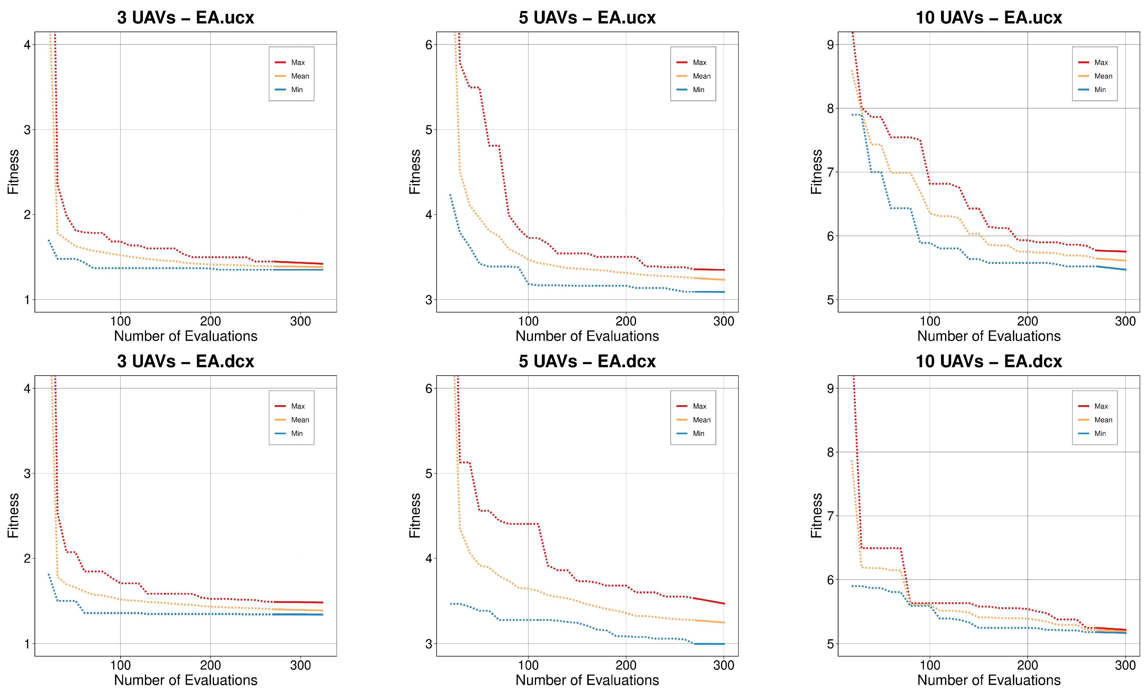
The convergence of the evolutionary algorithms is presented in
Figure 10 where the maximum, mean, and minimum fitness values were plotted as curves. At the end of each line, a continue trace represents the LS stage where the extra improvement achieved at the end of the algorithm execution is clearly shown. Using our hybrid approach resulted in achieving better solutions with a minimal effort (evaluations) as the LS only explores the best solution’s neighbourhood. The late improvement shown by the plots confirms the utility of our approach to improve the EA’s solutions.
5.3. Simulation Results
After the optimisation stage, we have tested the best configurations calculated by the algorithms in 90 unseen scenarios to address the robustness of each optimisation result. The obtained values are shown in
Table 4 where the measured distance to the rogue drone (Drd★) is detailed, as well as the precision of the final shape achieved, indicating the percentage of UAVs presenting final positions with a five-percent deviation from the desired five-metre radius, and also a less restrictive condition, i.e., ten percent.
It can be seen that a swarm of three UAVs achieved competitive results by using the three best configurations when tested on the 90 unseen scenarios, evidencing that it is the easiest of the case studies analysed. However, the swarm of five UAVs did perform differently, as only the configuration obtained by EA.dcx achieved the best results with 100% of UAVs placed into the five-percent tolerance at the end of the formation, followed by RS and EA.ucx (56.7% and 47.8%, respectively). Surprisingly, the configuration achieved by RS placed more UAVs in a stable shape than the EA.ucx’s, given insights of a possible overfitting as EA.ucx did improve RS during the optimisation process. We believe that this situation may be improved by choosing different optimisation scenarios (diversity) or a bigger number of them, although this would imply the use of far more computational resources.
Finally, in the most complex case study (10 UAVs), EA.ucx presented the most accurate results (93.3% of scenarios) followed by EA.dcx (51.1%), both arranging the UAVs in formations with a precision higher than 90%. The best configuration achieved by RS for 10 UAVs was unable to achieve precise spheric shape in any scenario. Due to the high complexity of this case study, no configuration obtained formations within plus/minus five-percent tolerance.
From the metrics obtained after testing the best configurations on 90 unseen scenarios per case study, we can see that three UAVs do not require a very fine tuning of their parameters as formations were always achieved, even when using the configuration found by RS. When the problem becomes more difficult, only EA.dcx finds a configuration for five UAVs that obtains 100% of successful formations (plus/minus 5% accuracy). This completely discards RS as an option, and leaves EA.ucx to be used for less precise formations. Finally, in the most complex case study, i.e., 10 UAVs, only formations with a 10% accuracy were possible, with EA.ucx being the best choice for that (93.3% of the testing scenarios). This does not mean that it underperformed in the remaining scenarios. On the contrary, the reported minimum and maximum distances to the centre (Drd★), show that despite the precision loss, the UAVs are still surrounding the rogue drone. This study thus confirms the necessity of testing the results from the optimisation of a given set of scenarios on different unseen conditions which, in the end, could give some insight about the robustness of the system.
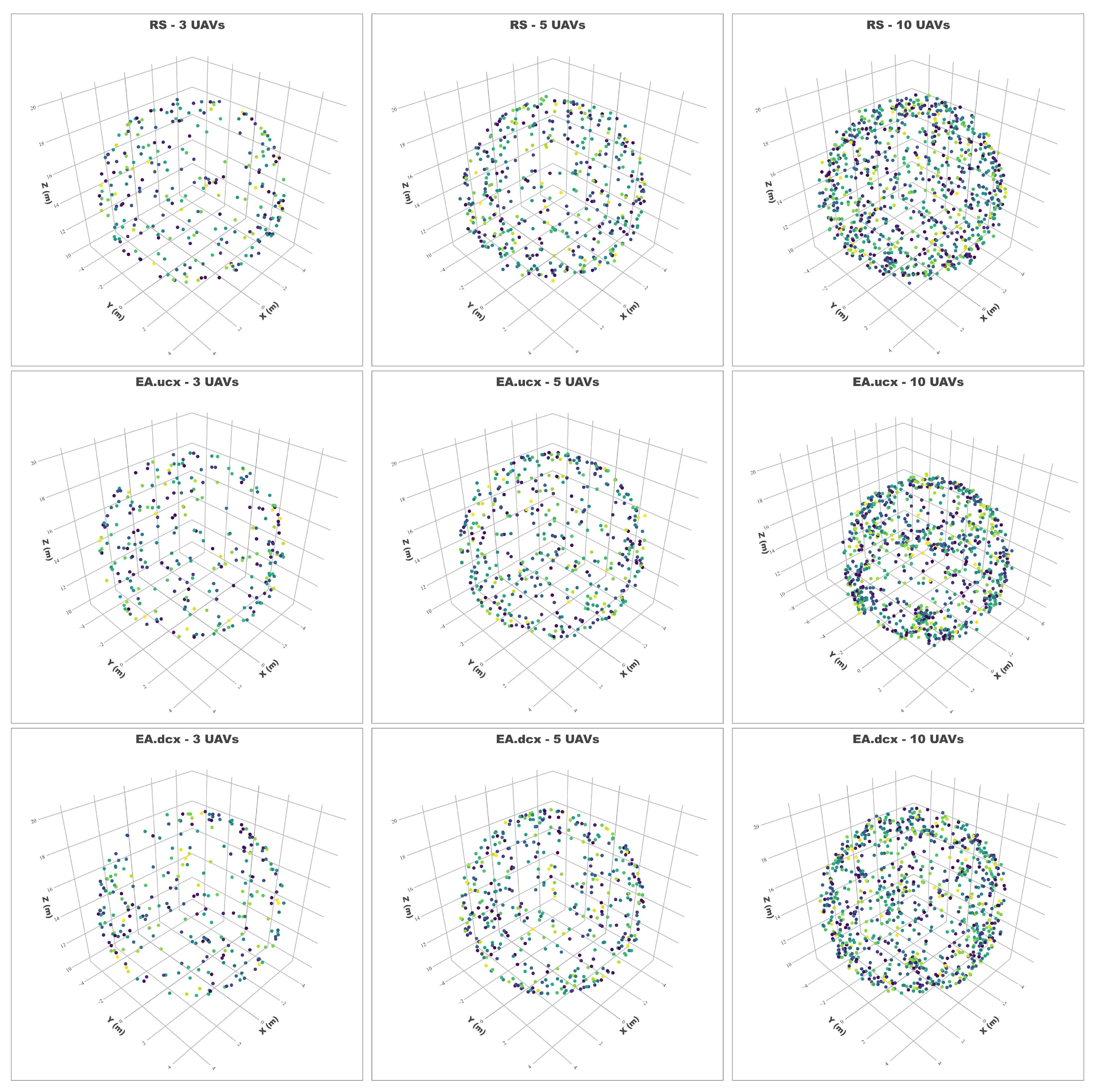
As a complement to the results presented in
Table 4,
Figure 11 shows the final positions of all the UAVs in the 90 scenarios per case study and algorithm. Despite the fact that it is hard to visualise a 3D representation of the swarm members, all the graphs show a sphere-like shape in contrast with the initial positions depicted in
Figure 6.
6. Conclusions
In this article, we have proposed an optimisation algorithm and tested two different crossover operators to optimise the configuration of a swarm of autonomous UAVs when performing a formation surrounding a rogue drone. This is a complex problem wherein the swarm members use the novel distributed formation algorithm (DFA3) to self-organise and achieve the desired formation by using only communication beacons and a set of parameters. Hence, the calculation of these optimal parameters is challenging and prone to be done by using an intelligent algorithm such as a metaheuristic. Consequently, we have designed a hybrid EA built with a genetic algorithm and a local search stage at the end of the optimisation process to better exploit the best solution found by the first stage. The optimisation results showed that the proposed EA outperformed the RS results in all the case studies as expected, whereas for swarms of three and five UAVs, both tested EAs (EA.ucx using a uniform crossover operator and EA.dcx using a drone crossover operator) presented similar results. In the most difficult case study featuring 10 UAVs, the proposed alternative algorithm (EA.dcx) outperformed the other two, achieving better fitness values, which were statistically validated. Having obtained the optimal parameter set for each swarm, we have tested them on 90 unseen scenarios (UAVs in different initial positions) to address the robustness of the swarm configurations.
From our results, we can conclude that the formation problem using the proposed DFA3 is viable and it achieves competitive results when using an intelligent algorithm, e.g., EA, to calculate the system parameters. The two EA variants proposed performed well in most of the 300 tested scenarios although some overfitting was observed. Hence, the proposed DFA3 and the proposed hybrid EAs are capable of achieving accurate formations by using three UAVs and five UAVs, while for swarms of 10 UAVs, successful formations were built in 95% of cases with plus/minus 10% accuracy.
As a matter of future work, it would be interesting to address more case studies as well as the main issue observed, the aforementioned overfitting, by using a higher number of optimisation scenarios or even using a different technique such as k-fold cross validation. Because the number of experiments is limited by the required simulation time (if we want realistic simulations), we would like to study the use of surrogates to speed up the optimisation process and then validate the results by using heavy simulations. We plan to study robot failures to assess how the swarm rebuilds a broken formation using the initial configuration, e.g., eight- or nine-UAV swarm using the parameters calculated for 10 UAVs. Different formation shapes are also to be studied and the ways the DFA3 can be modified to achieve such other formations. Currently, we are working in the implementation of the DFA3 by using real UAV robots to validate in vivo the results we have observed and presented in vitro.


