
A CSI-Based Multi-Environment Human Activity Recognition Framework

 , , , and
Abstract
:1. Introduction
- We addressed a multi-environment human activity identification problem.
- We evaluated the proposed system using a leave-one-subject-out manner in which no activity trace from that subject is used to train the classification model.
- A novel segmentation method to remove the part of the signal that contains no-movements is developed.
- A methodology for denoising the collected CSI values, which are obtained from the Wi-Fi exchanged packets, is introduced.
- A large number of handcrafted features were investigated to determine their effectiveness in recognizing the different performed human activities in a multi-environment domain.
- To add to the credibility of this work, ample experiments are conducted using the publicly available dataset to demonstrate the effectiveness of the proposed methodology in determining the differently performed human activities.
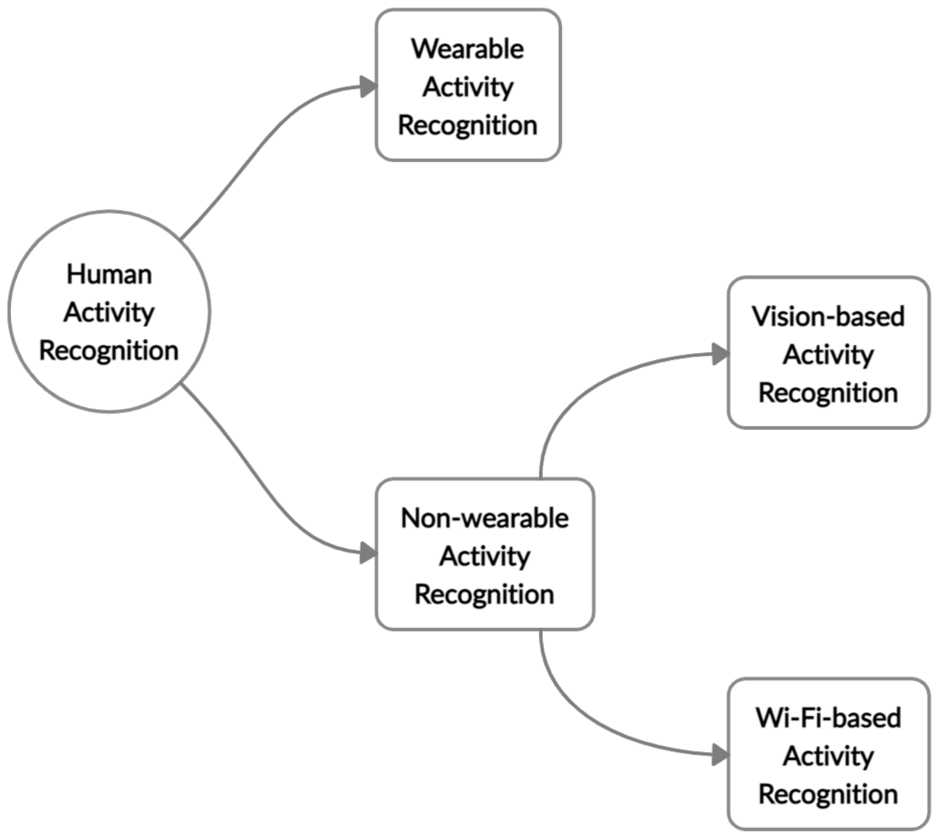
1.1. Related Work
1.1.1. Wearable Activity Recognition
1.1.2. Non-Wearable Activity Recognition Approaches
1.2. Background
2. Materials and Methods
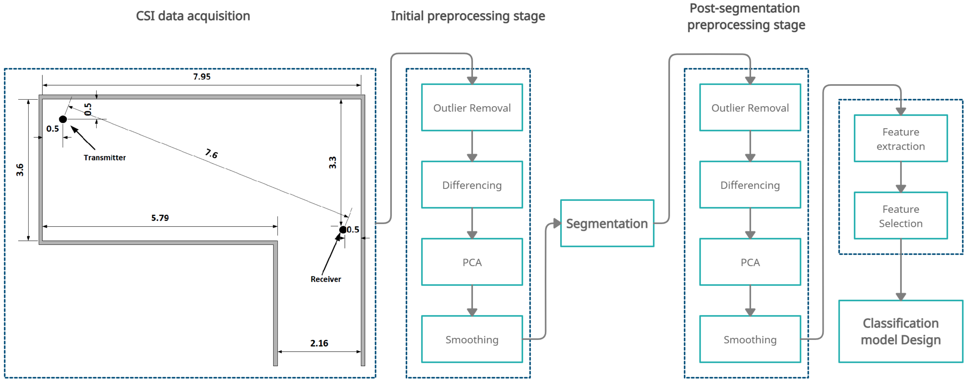
2.1. Experimental Setup
2.2. Environment Description
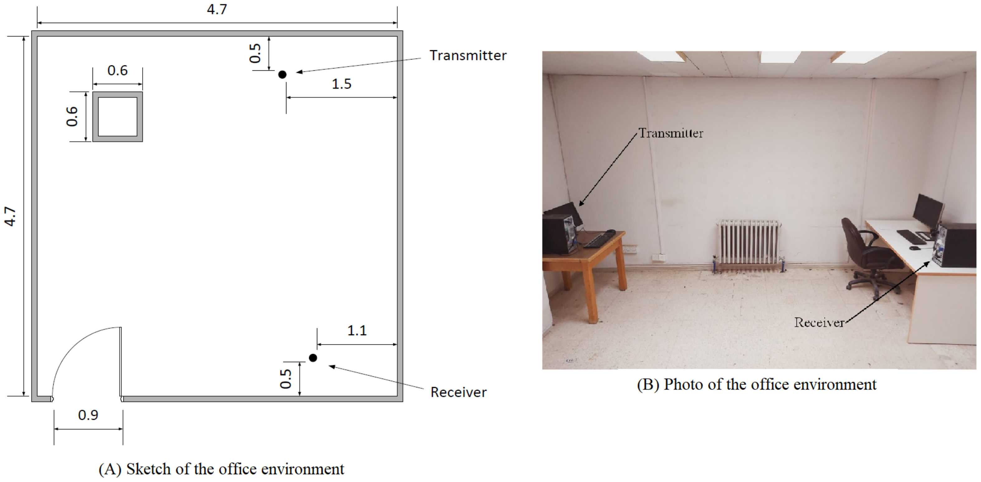
2.2.1. The Office Environment
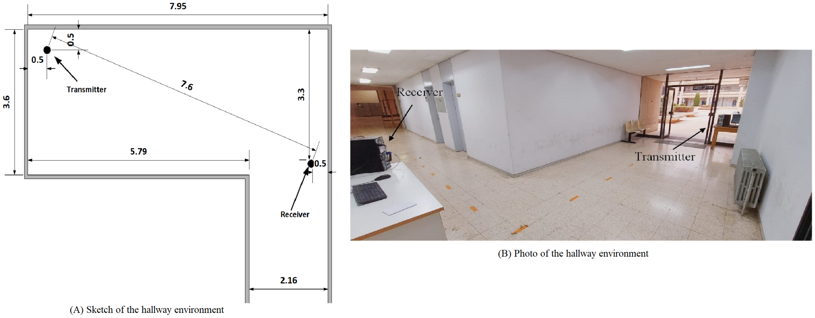
2.2.2. The Hallway Environment
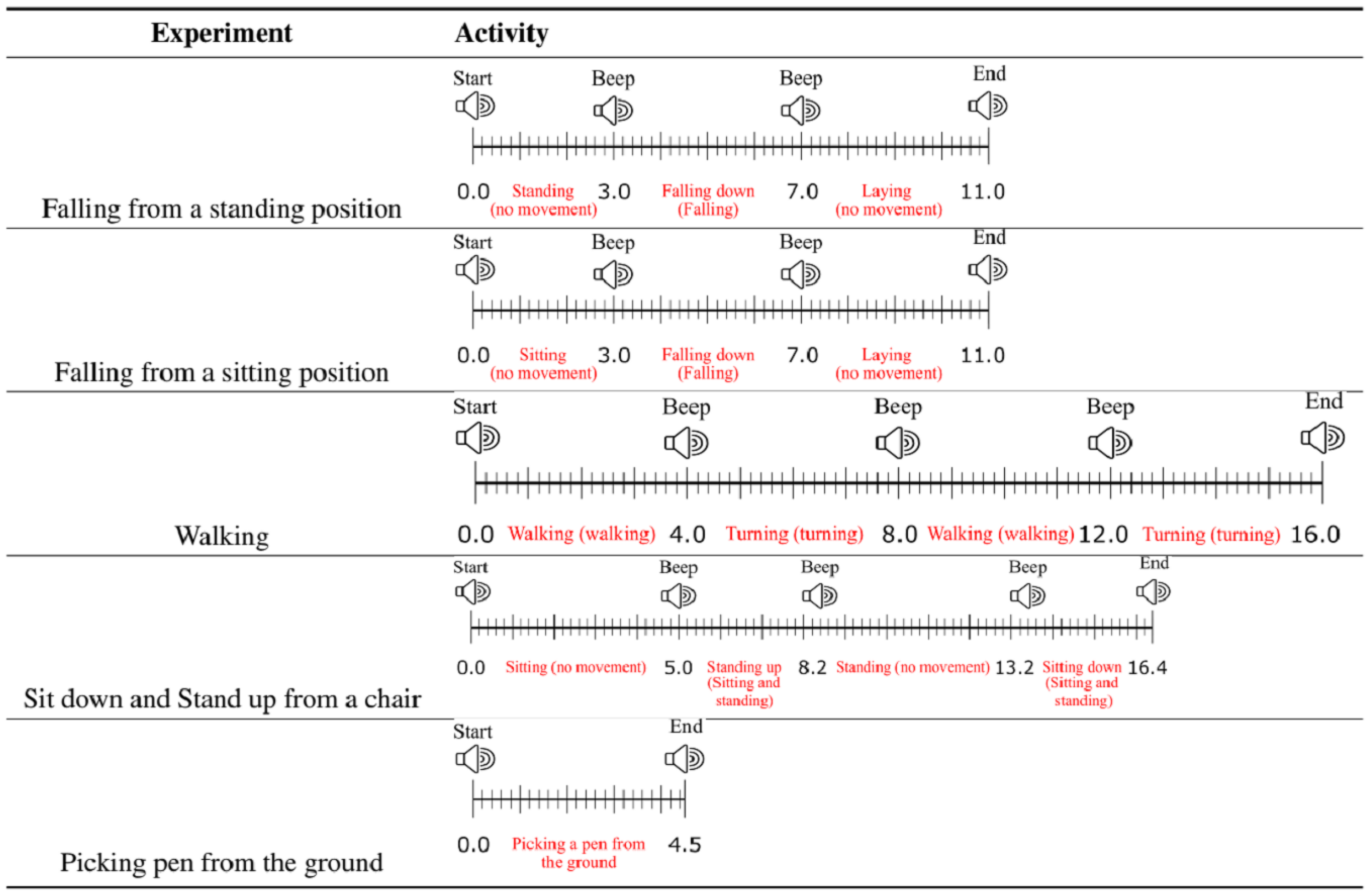
2.3. Activity Description and Data Collection
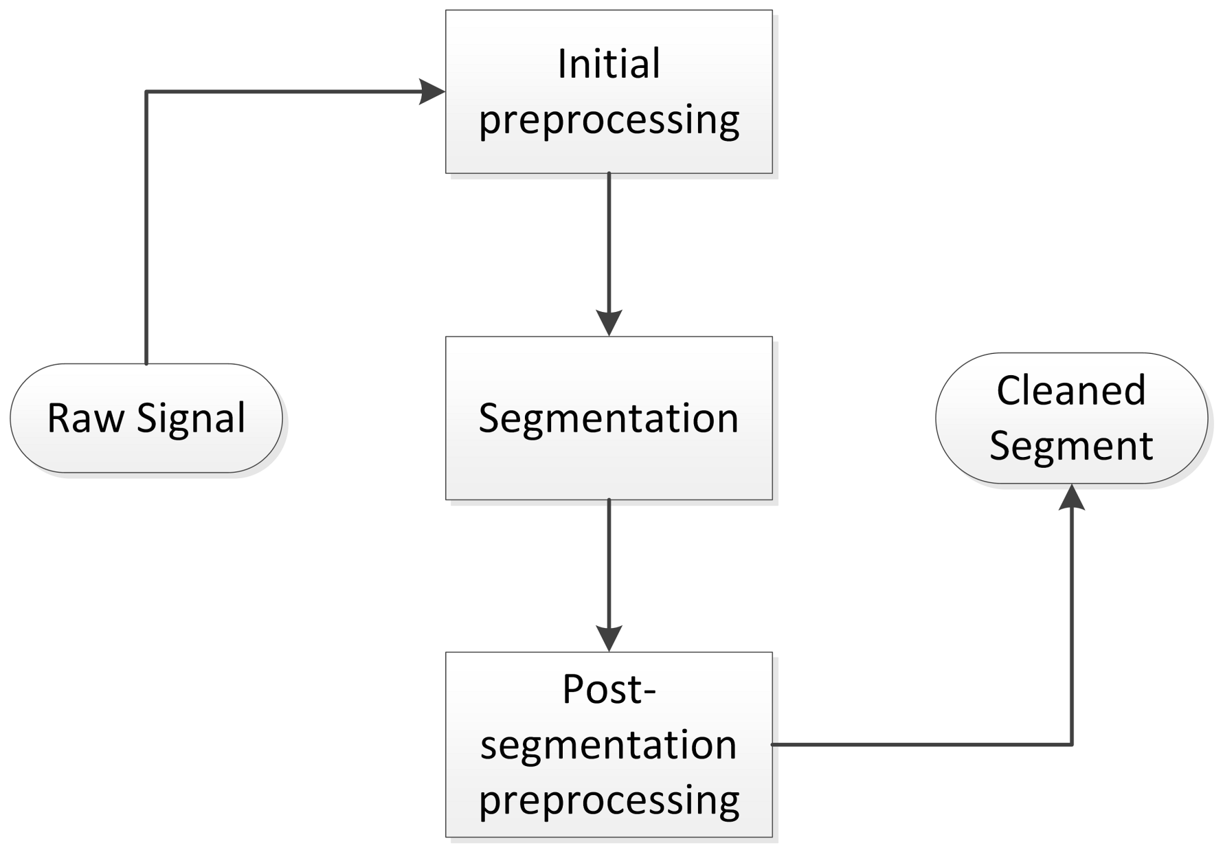
2.4. Data Pre-Processing
2.4.1. Initial Preprocessing Stage
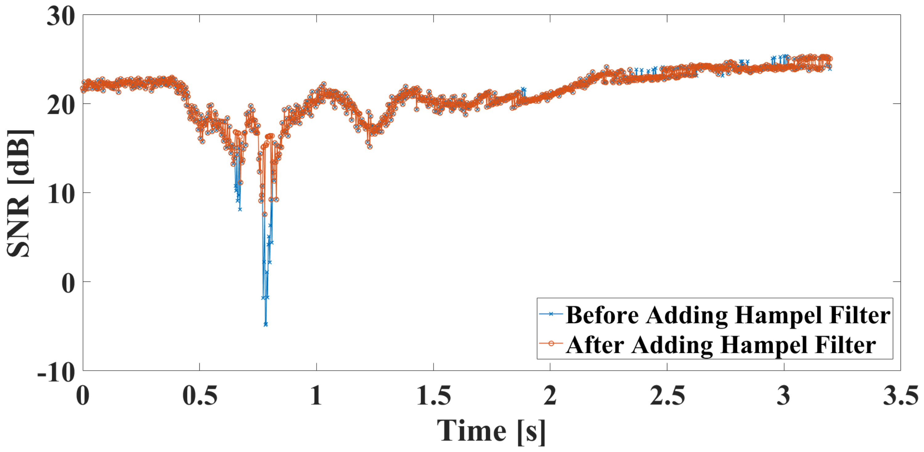
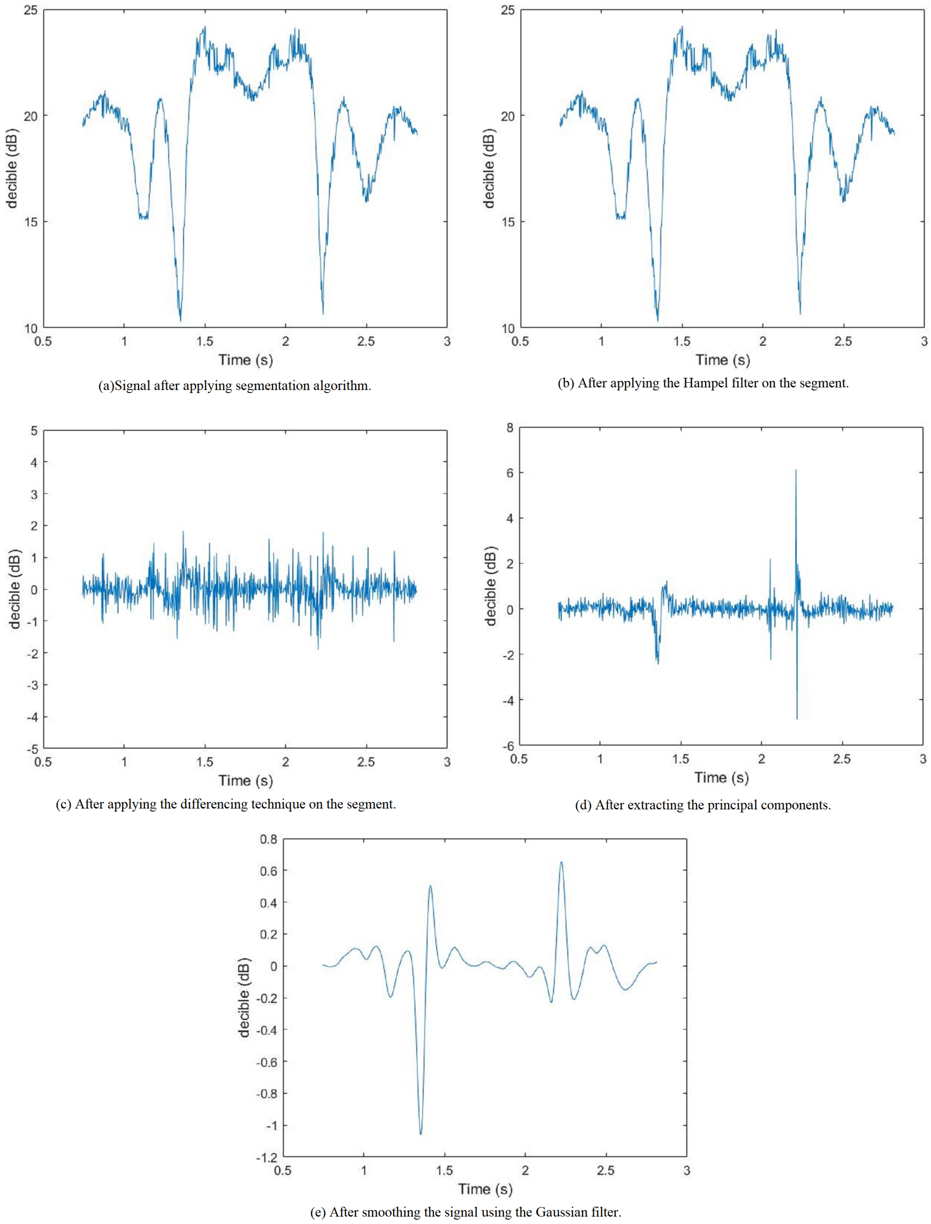
- Outliers Removal: This technique is used to remove any value that can be considered as an outlier. Outlier values can occur for several reasons: the noise present in the environment incorrect hardware reading, and the sudden change in the environment are possible reasons for such outliers. To exclude these outliers, the Hampel filter [42] was used. The Hampel filter utilizes a sliding window that scans the CSI signals and removes any reading that is more than three times the standard deviation () by replacing that value with the mean of the values within the sliding window. An example of a processed signal using the Hampel filter is shown in Figure 8.
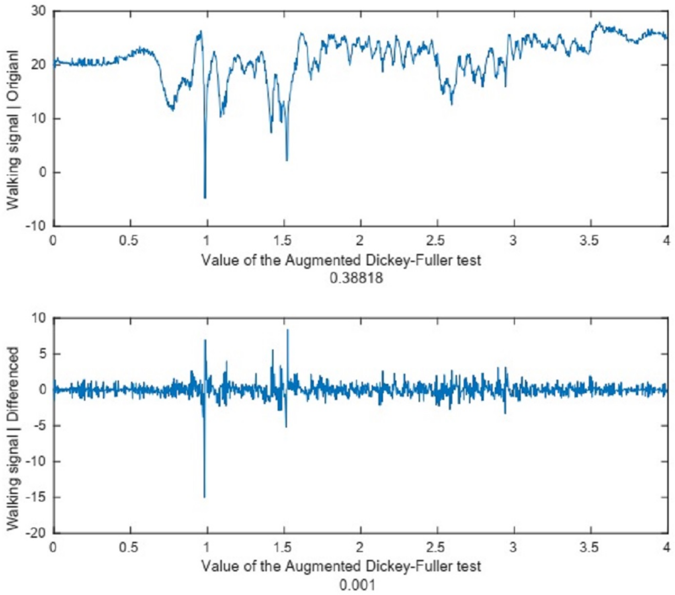
- Converting to Stationary signal: A stationary signal is a term used to describe a signal with constant or slowly changing statistical properties as discussed in [43]. In this work, the signals we are dealing with are all non-stationary signals [44]. The term non-stationary signal refers to a signal with statistical values (mean, median, variance) that are changing over time. To transform the non-stationary signal into a stationary signal, the differencing procedure can be applied by subtracting each value of the time-series signal from the one before it as follows [45]:where represents a reading at time t, represents the previous data reading, and represents the new reading that will replace .To determine if this step is necessary or not, we performed the Augmented Dickey-Fuller (ADF) test [46]. The ADF test determines if the signal at hand is stationary or not by testing the null hypothesis (), which refers to a non-stationary signal. To determine if the signal is stationary, we look for a p-value less than or equal to 0.05. An example of the performed ADF test is provided in the “Before Segmentation Processing” Section.
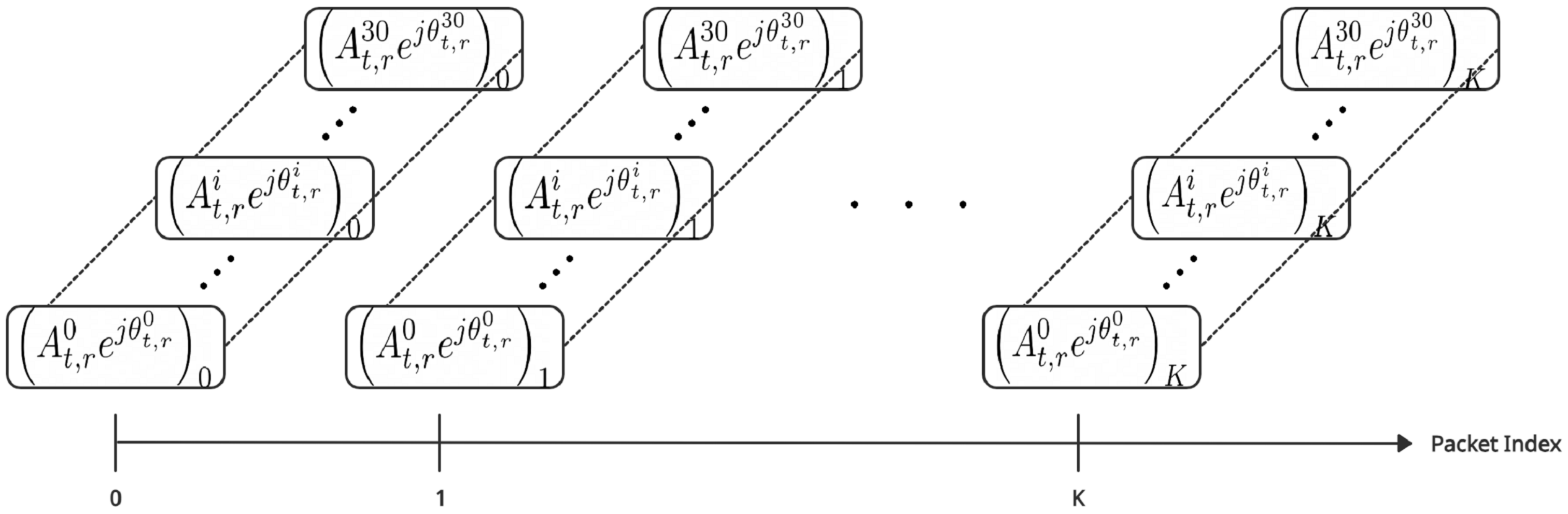
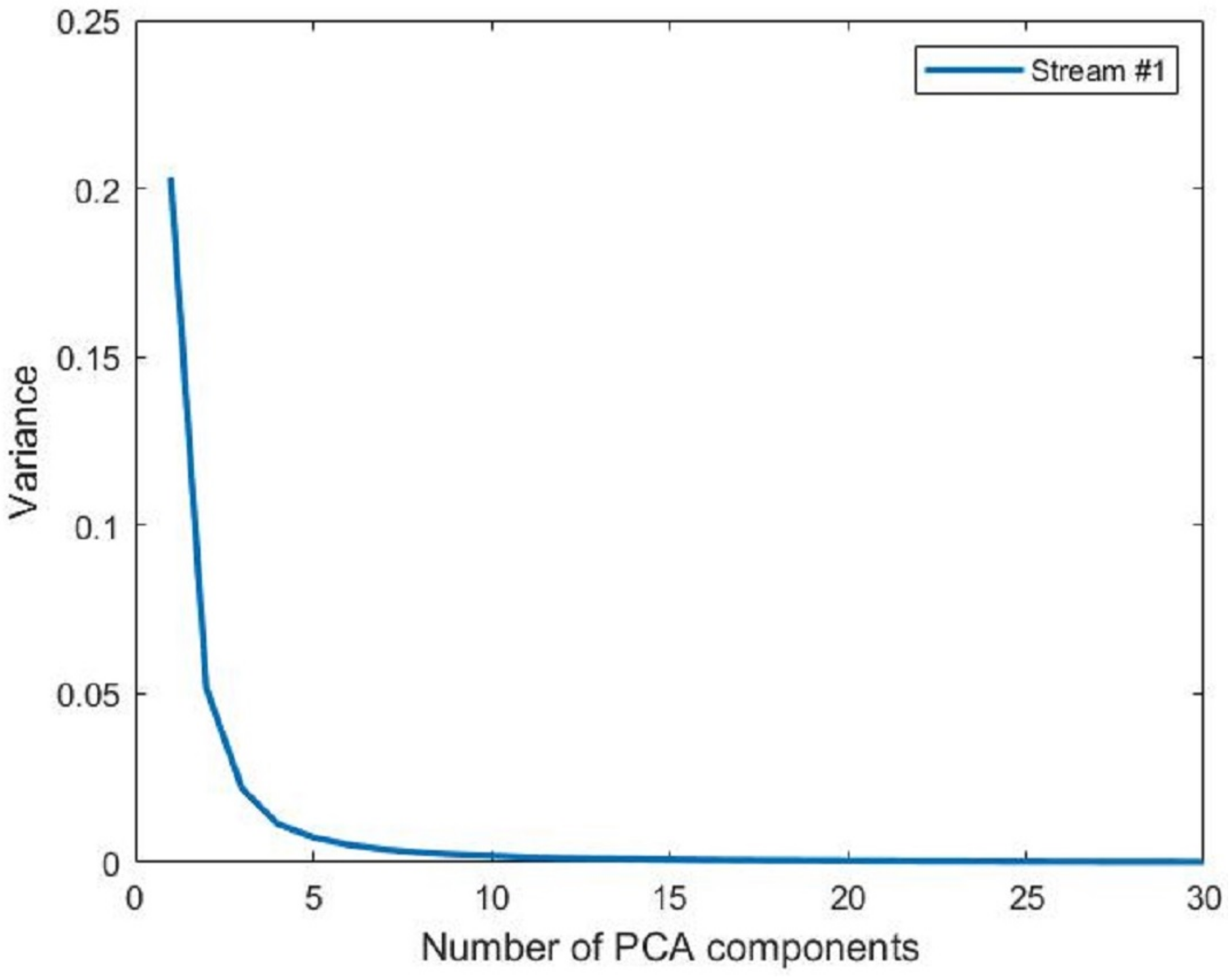
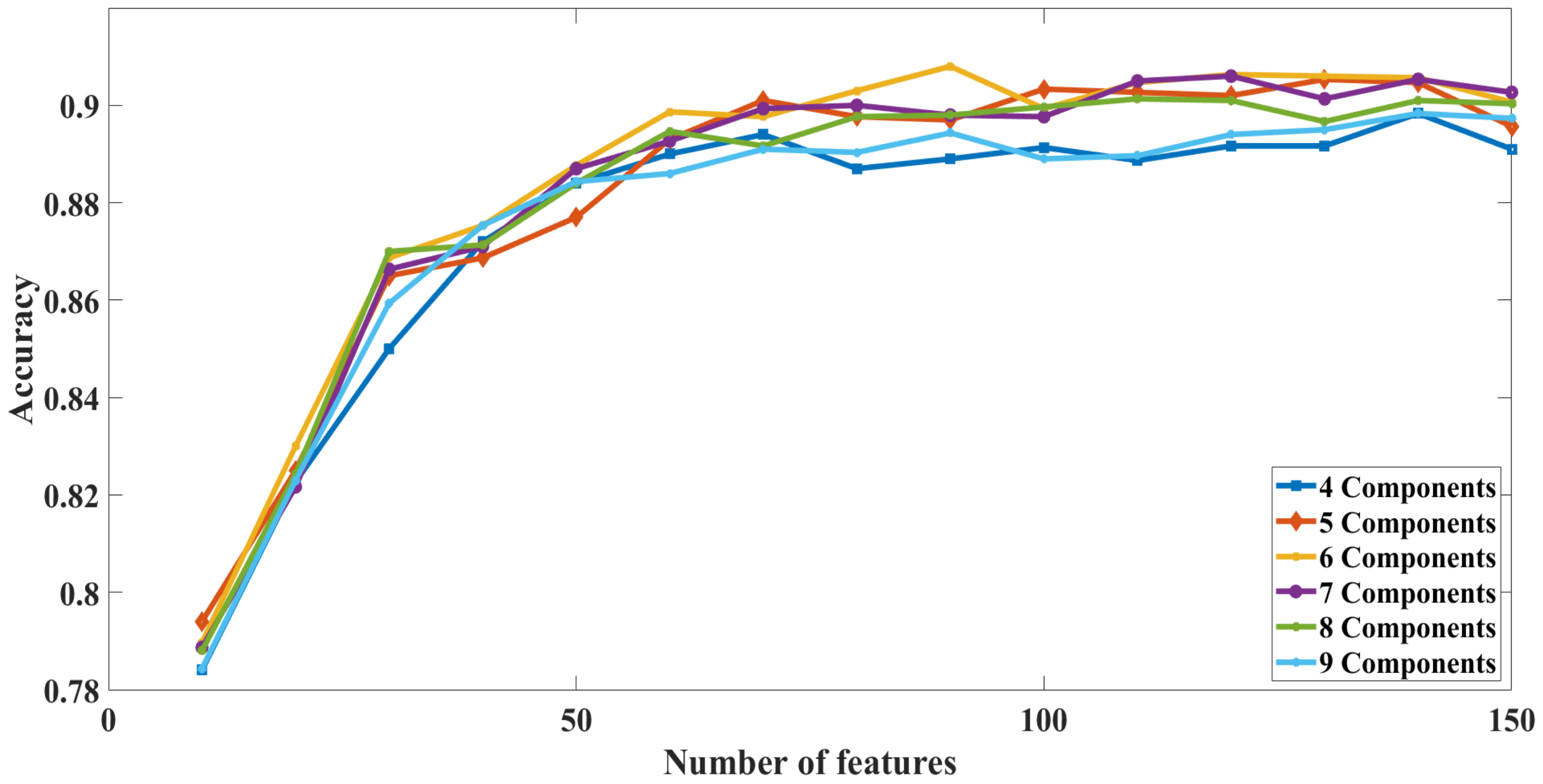
- Data Reduction: Each receiving antenna records 30 CSI-subcarriers in each of the communication channels. The use of all 30 subcarriers will create a strain on the system. To reduce the number of signals to be analyzed and at the same time to retain the valuable information in these signals, we use the Principal Component Analysis (PCA) [47], which is considered a dimensionality reduction method. To determine the number of principal components to be selected, the following two metrics were considered: (1) The data variance in the selected principal components; (2) The errors in the segmentation process. A detailed description of each metrics is provided in the “Before Segmentation Processing” section.
- Signal Smoothing: For each of the principal components we selected in the previous stage, we need to reduce the noise in that signal through a smoothing technique. One of the most known techniques to remove such noise, especially in the area of image processing, is known as Gaussian filtering [48]. The basic approach to smooth a signal is by defining a Gaussian window with the point we want to smooth in the middle of the window. To generate the smoothed point, each actual data point has a related Gaussian weight (the summation for the weights must be equal to 1). These Gaussian weights are then multiplied by the actual data values, and the summation of the multiplication results is assumed to be the new value after smoothing.
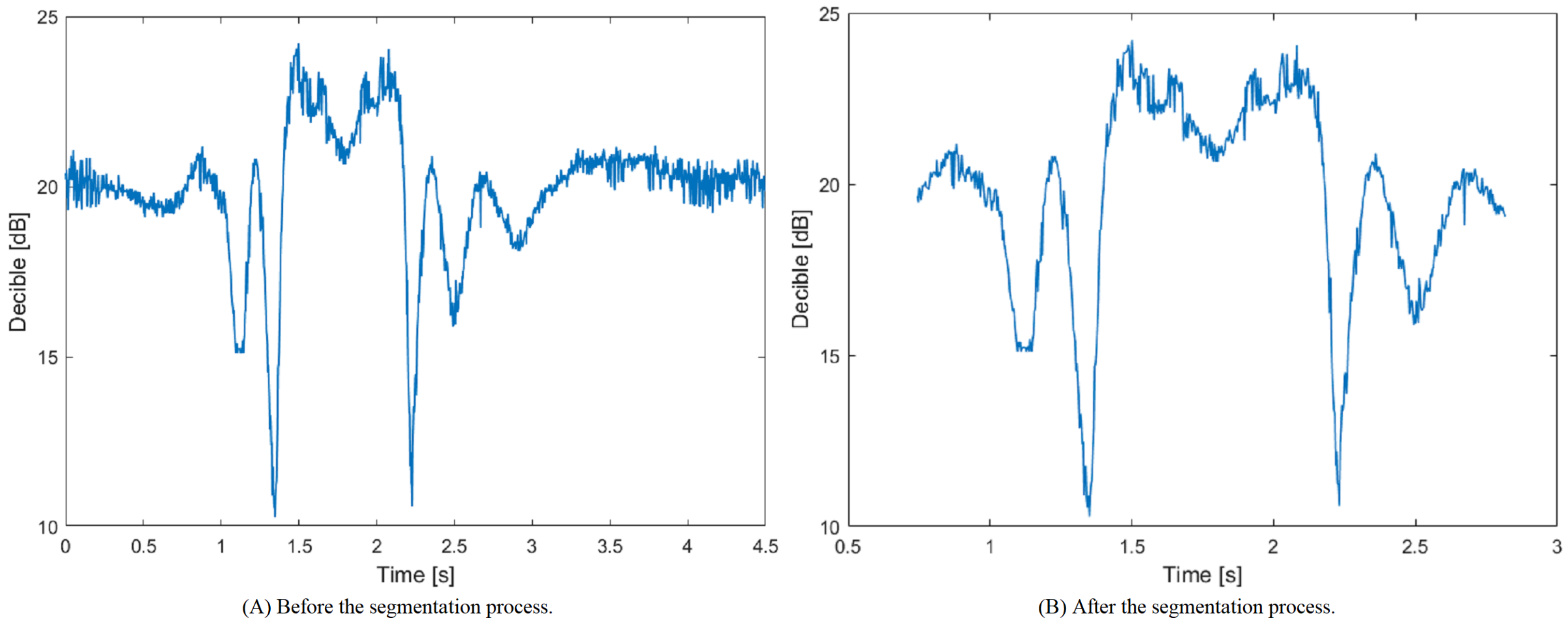
2.4.2. The Segmentation Stage
2.4.3. The Post-Segmentation Preprocessing Stage
- The first interval represents the interval until the subject begins the activity. During this time interval, we expect the subject to remain stationary;
- the second interval represents the segment in which the activity occurred; and
- the third interval represents the interval from the end of the activity until the subject is instructed to finish the activity. Similar to the first interval, the subject is expected to remain stationary during the third interval.
2.4.4. Feature Extraction
2.4.5. Feature Selection
2.4.6. Classification Model
3. Results
3.1. Data Preparation
3.1.1. Initial Preprocessing Stage
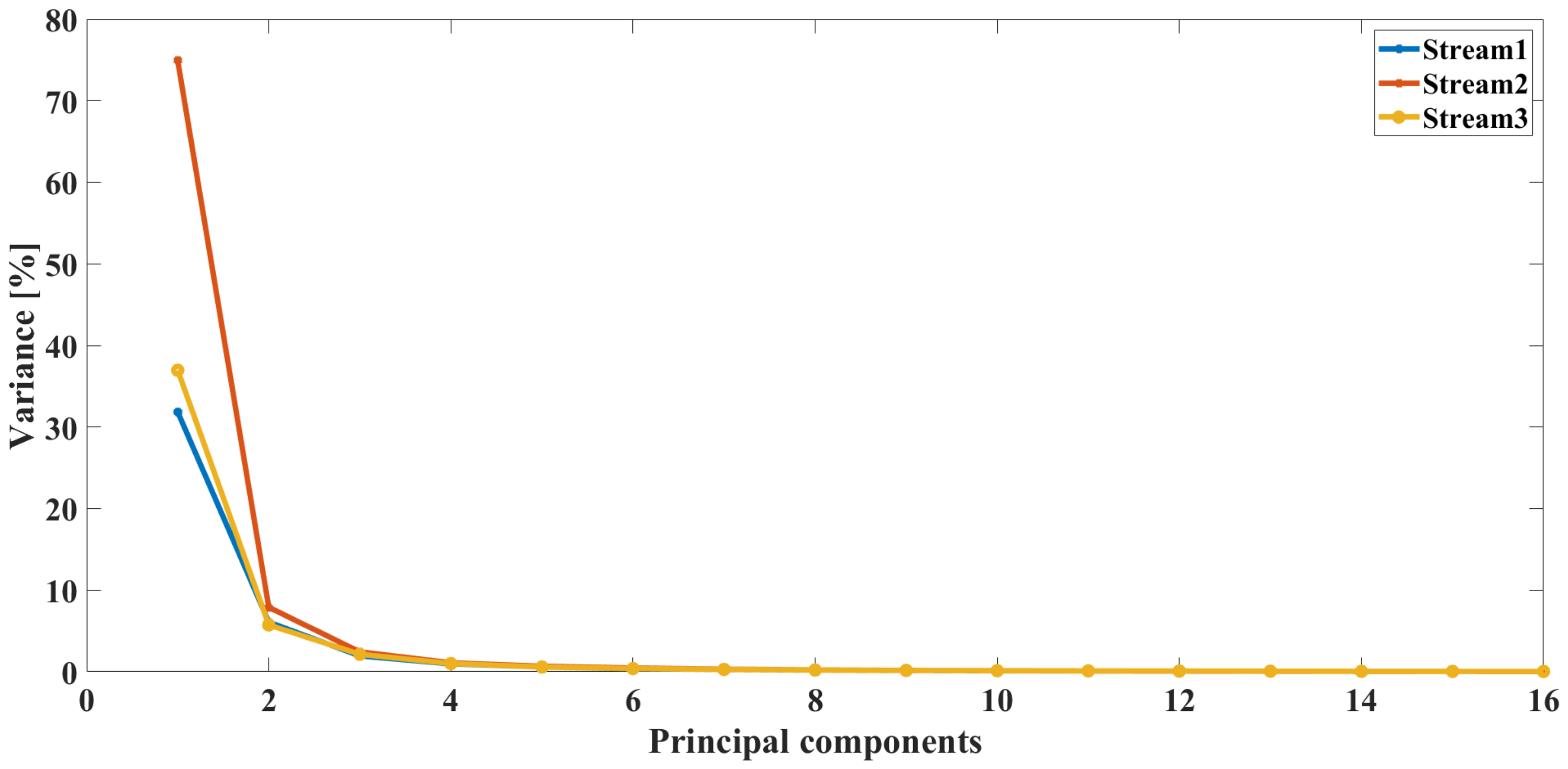
- The variance in the principal components. For this metric, we calculated the variance of the data in each of the principal components. Figure 11 shows the variance contained in each of the principal components generated from the first stream of the office environment. It shows no meaning in using all the principal components since there is no data variance in the components above the 10th component. We found out that 98% of the data variance is contained in the first eight principal components.
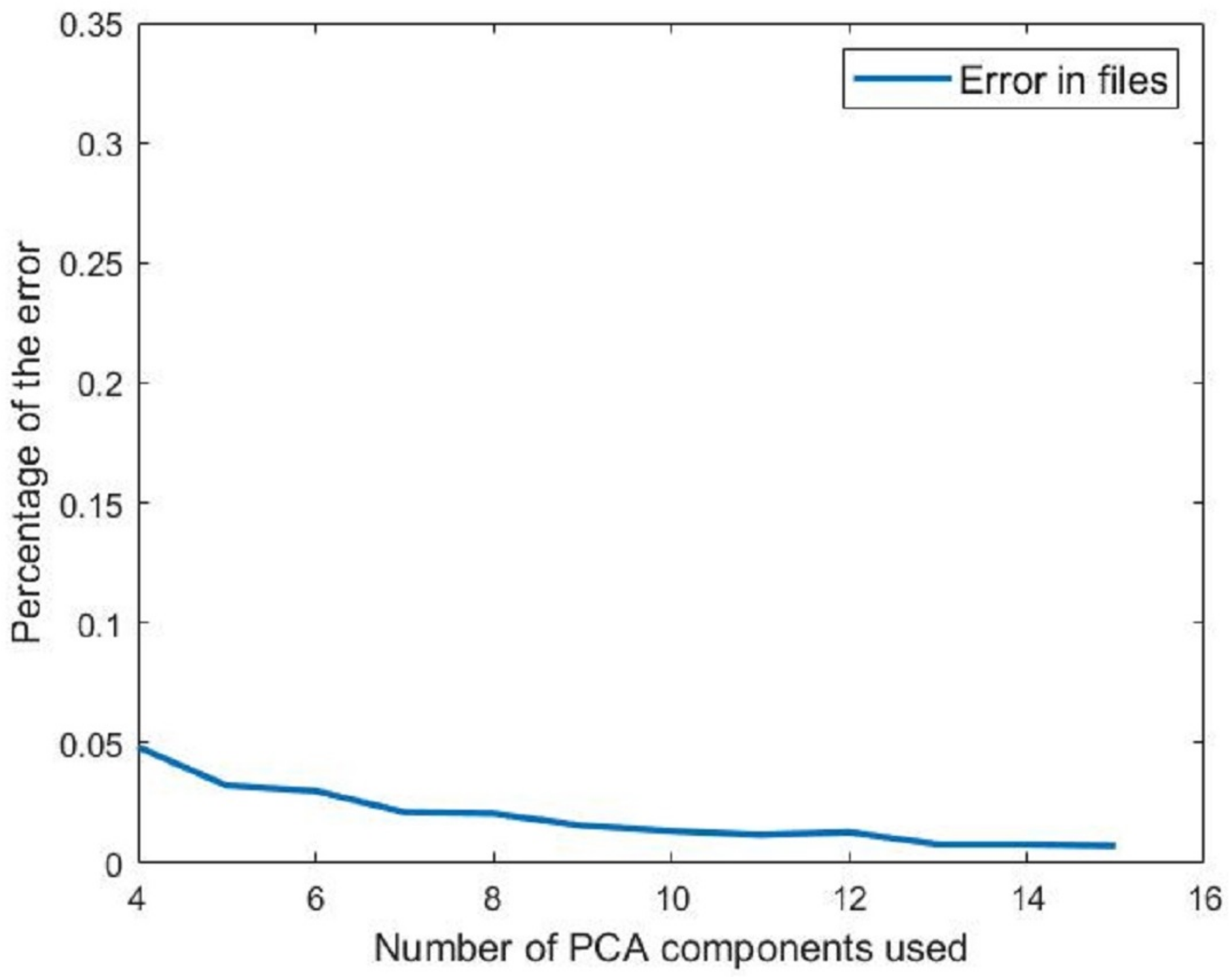
- The error in activity segmentation. For this metric, we performed the segmentation procedure using various principal component combinations. We started with four components and stopped when we reached 15 components since most of the data are contained in the earliest components. The segmentation algorithm may lead to a segmentation error if it cannot determine the segment’s starting or ending points. This latter condition is used as a metric to determine how many principal components to use. Figure 12 shows the percentage of recorded activities that the segmentation algorithm was unable to extract a segment from. If we selected eight principal components, as the first evidence suggested, only 1% of the activities will not be segmented successfully. Such errors will be handled after the segmentation procedure as described in the “segmentation” Section.
3.1.2. Segmentation
- In the first case, the segmentation algorithm works correctly, and it was able to identify the start and the end of the activity within each of the communication streams. Thus, no further action is needed, and the starting and ending points are used to extract the segment;
- The second case happens when two streams are segmented successfully, while the third stream is not segmented. In this case, we take the average of the starting points from the two successful streams and the average of the ending points from the two successful streams and use them as the starting and ending points for the third unsuccessful stream;
- The third case occurs when only one stream is segmented successfully, while no segments were detected for the other two streams. In such a case, we assume that the segments for the two streams are the same as the segment for the stream we successfully found the segment in it; and
- The last case comes about when the segmentation algorithm does not successfully extract the activity segment in any of the streams. The index that represents the beginning of the segment can then be computed as follows:where S is the index of the segment beginning, H is the point associated with the highest value of the signal, and L is the point associated with the lowest value of the signal.On the other hand, the calculations for the segment endpoint are expressed as follows:where E is the index of the segment end and A represents the index of the end of the signal. In other words, the segment end index is the midpoint between the end of the signal and the furthest occurrence of either the highest-peak or the lowest-peak values in that signal.
3.1.3. Post-Segmentation Preprocessing Stage
3.2. Feature Extraction and Selection
3.3. Classification Results
3.3.1. Results of the First Evaluation Scenario
3.3.2. Results of the Second Evaluation Scenario
3.3.3. Results of the Third Evaluation Scenario
3.3.4. Results of the Fourth Evaluation Scenario
3.3.5. Results of the Fifth Evaluation Scenario
4. Discussion
4.1. Performance Comparison
4.2. Limitations and Future Work
5. Conclusions
Author Contributions
Funding
Institutional Review Board Statement
Informed Consent Statement
Data Availability Statement
Conflicts of Interest
References
- Husen, M.N.; Lee, S. Indoor human localization with orientation using WiFi fingerprinting. In Proceedings of the 8th International Conference on Ubiquitous Information Management and Communication, Siem Reap, Cambodia, 9–11 January 2014; pp. 1–6. [Google Scholar]
- Fu, Z.; Xu, J.; Zhu, Z.; Liu, A.X.; Sun, X. Writing in the air with WiFi signals for virtual reality devices. IEEE Trans. Mob. Comput. 2018, 18, 473–484. [Google Scholar] [CrossRef]
- Jordao, A.; Torres, L.A.B.; Schwartz, W.R. Novel approaches to human activity recognition based on accelerometer data. Signal Image Video Process. 2018, 12, 1387–1394. [Google Scholar] [CrossRef]
- Hussain, T.; Maqbool, H.F.; Iqbal, N.; Khan, M.; Dehghani-Sanij, A.A. Computational model for the recognition of lower limb movement using wearable gyroscope sensor. Int. J. Sens. Netw. 2019, 30, 35–45. [Google Scholar] [CrossRef]
- Jain, A.; Kanhangad, V. Human activity classification in smartphones using accelerometer and gyroscope sensors. IEEE Sens. J. 2017, 18, 1169–1177. [Google Scholar] [CrossRef]
- Jalal, A.; Kamal, S.; Azurdia-Meza, C.A. Depth maps-based human segmentation and action recognition using full-body plus body color cues via recognizer engine. J. Electr. Eng. Technol. 2019, 14, 455–461. [Google Scholar] [CrossRef]
- Vemulapalli, R.; Arrate, F.; Chellappa, R. Human action recognition by representing 3d skeletons as points in a lie group. In Proceedings of the IEEE Conference on Computer Vision and Pattern Recognition, Columbus, OH, USA, 23–28 June 2014; pp. 588–595. [Google Scholar]
- Mohamed, S.E. Why the Accuracy of the Received Signal Strengths as a Positioning Technique was not accurate? Int. J. Wirel. Mob. Netw. (IJWMN) 2011, 3, 69–82. [Google Scholar] [CrossRef]
- Wang, X.; Yang, C.; Mao, S. ResBeat: Resilient breathing beats monitoring with realtime bimodal CSI data. In Proceedings of the GLOBECOM 2017—2017 IEEE Global Communications Conference, Singapore, 4–8 December 2017; pp. 1–6. [Google Scholar]
- Xu, Y.; Yang, W.; Chen, M.; Chen, S.; Huang, L. Attention-Based Gait Recognition and Walking Direction Estimation in Wi-Fi Networks. IEEE Trans. Mob. Comput. 2020, 21, 465–479. [Google Scholar] [CrossRef]
- Khalifa, S.; Lan, G.; Hassan, M.; Seneviratne, A.; Das, S.K. Harke: Human activity recognition from kinetic energy harvesting data in wearable devices. IEEE Trans. Mob. Comput. 2017, 17, 1353–1368. [Google Scholar] [CrossRef]
- Altun, K.; Barshan, B.; Tunçel, O. Comparative study on classifying human activities with miniature inertial and magnetic sensors. Pattern Recognit. 2010, 43, 3605–3620. [Google Scholar] [CrossRef]
- Zubair, M.; Song, K.; Yoon, C. Human activity recognition using wearable accelerometer sensors. In Proceedings of the 2016 IEEE International Conference on Consumer Electronics-Asia (ICCE-Asia), Seoul, Korea, 26–28 October 2016; pp. 1–5. [Google Scholar]
- Ugulino, W.; Cardador, D.; Vega, K.; Velloso, E.; Milidiú, R.; Fuks, H. Wearable computing: Accelerometers’ data classification of body postures and movements. In Brazilian Symposium on Artificial Intelligence; Springer: Berlin, Germany, 2012; pp. 52–61. [Google Scholar]
- Badawi, A.A.; Al-Kabbany, A.; Shaban, H. Multimodal human activity recognition from wearable inertial sensors using machine learning. In Proceedings of the 2018 IEEE-EMBS Conference on Biomedical Engineering and Sciences (IECBES), Sarawak, Malaysia, 3–6 December 2018; pp. 402–407. [Google Scholar]
- Lu, Y.; Wei, Y.; Liu, L.; Zhong, J.; Sun, L.; Liu, Y. Towards unsupervised physical activity recognition using smartphone accelerometers. Multimed. Tools Appl. 2017, 76, 10701–10719. [Google Scholar] [CrossRef]
- Janidarmian, M.; Roshan Fekr, A.; Radecka, K.; Zilic, Z. A comprehensive analysis on wearable acceleration sensors in human activity recognition. Sensors 2017, 17, 529. [Google Scholar] [CrossRef] [PubMed]
- Deep, S.; Zheng, X. Leveraging CNN and transfer learning for vision-based human activity recognition. In Proceedings of the 2019 29th International Telecommunication Networks and Applications Conference (ITNAC), Auckland, New Zealand, 27–29 November 2019; pp. 1–4. [Google Scholar]
- Jobanputra, C.; Bavishi, J.; Doshi, N. Human Activity Recognition: A Survey. Procedia Comput. Sci. 2019, 155, 698–703. [Google Scholar] [CrossRef]
- Ji, X.; Cheng, J.; Feng, W.; Tao, D. Skeleton embedded motion body partition for human action recognition using depth sequences. Signal Process. 2018, 143, 56–68. [Google Scholar] [CrossRef]
- Wang, J.; Liu, Z.; Wu, Y.; Yuan, J. Mining actionlet ensemble for action recognition with depth cameras. In Proceedings of the 2012 IEEE Conference on Computer Vision and Pattern Recognition, Providence, RI, USA, 16–21 June 2012; pp. 1290–1297. [Google Scholar]
- Oreifej, O.; Liu, Z. Hon4d: Histogram of oriented 4d normals for activity recognition from depth sequences. In Proceedings of the IEEE Conference on Computer Vision and Pattern Recognition, Portland, OR, USA, 23–28 June 2013; pp. 716–723. [Google Scholar]
- Li, W.; Zhang, Z.; Liu, Z. Action recognition based on a bag of 3d points. In Proceedings of the 2010 IEEE Computer Society Conference on Computer Vision and Pattern Recognition-Workshops, San Francisco, CA, USA, 13–18 June 2010; pp. 9–14. [Google Scholar]
- Xia, L.; Chen, C.C.; Aggarwal, J.K. View invariant human action recognition using histograms of 3d joints. In Proceedings of the 2012 IEEE Computer Society Conference on Computer Vision and Pattern Recognition Workshops, Providence, RI, USA, 16–21 June 2012; pp. 20–27. [Google Scholar]
- Gu, Y.; Liu, T.; Li, J.; Ren, F.; Liu, Z.; Wang, X.; Li, P. Emosense: Data-driven emotion sensing via off-the-shelf wifi devices. In Proceedings of the 2018 IEEE International Conference on Communications (ICC), Kansas City, MO, USA, 20–24 May 2018; pp. 1–6. [Google Scholar]
- Wang, X.; Yang, C.; Mao, S. PhaseBeat: Exploiting CSI phase data for vital sign monitoring with commodity WiFi devices. In Proceedings of the 2017 IEEE 37th International Conference on Distributed Computing Systems (ICDCS), Atlanta, GA, USA, 5–8 June 2017; pp. 1230–1239. [Google Scholar]
- Gu, Y.; Zhang, X.; Liu, Z.; Ren, F. WiFi-based Real-time Breathing and Heart Rate Monitoring during Sleep. arXiv 2019, arXiv:1908.05108. [Google Scholar]
- Alazrai, R.; Hababeh, M.; Alsaify, B.A.; Ali, M.Z.; Daoud, M.I. An End-to-End Deep Learning Framework for Recognizing Human-to-Human Interactions Using Wi-Fi Signals. IEEE Access 2020, 8, 197695–197710. [Google Scholar] [CrossRef]
- Alazrai, R.; Awad, A.; Alsaify, B.; Hababeh, M.; Daoud, M.I. A dataset for Wi-Fi-based human-to-human interaction recognition. Data Brief 2020, 31, 105668. [Google Scholar] [CrossRef]
- Cheng, L.; Wang, J. Walls Have No Ears: A Non-Intrusive WiFi-Based User Identification System for Mobile Devices. IEEE/ACM Trans. Netw. (TON) 2019, 27, 245–257. [Google Scholar] [CrossRef]
- Jakkala, K.; Bhuya, A.; Sun, Z.; Wang, P.; Cheng, Z. Deep CSI Learning for Gait Biometric Sensing and Recognition. arXiv 2019, arXiv:1902.02300. [Google Scholar]
- Wang, W.; Liu, A.X.; Shahzad, M.; Ling, K.; Lu, S. Device-free human activity recognition using commercial WiFi devices. IEEE J. Sel. Areas Commun. 2017, 35, 1118–1131. [Google Scholar] [CrossRef]
- Ding, J.; Wang, Y. WiFi CSI-Based Human Activity Recognition Using Deep Recurrent Neural Network. IEEE Access 2019, 7, 174257–174269. [Google Scholar] [CrossRef]
- Chen, Z.; Zhang, L.; Jiang, C.; Cao, Z.; Cui, W. WiFi CSI based passive human activity recognition using attention based BLSTM. IEEE Trans. Mob. Comput. 2018, 18, 2714–2724. [Google Scholar] [CrossRef]
- Yousefi, S.; Narui, H.; Dayal, S.; Ermon, S.; Valaee, S. A survey on behavior recognition using wifi channel state information. IEEE Commun. Mag. 2017, 55, 98–104. [Google Scholar] [CrossRef]
- Lagashkin, R. Human Localization and Activity Classification by Machine Learning on Wi-Fi Channel State Information. Master’s Thesis, School of Electrical Engineering, Aalto University, Espoo, Finland, 2020. [Google Scholar]
- Nee, R.V.; Prasad, R. OFDM for Wireless Multimedia Communications; Artech House, Inc.: London, UK, 2000. [Google Scholar]
- Marzetta, T.L.; Hochwald, B.M. Fast transfer of channel state information in wireless systems. IEEE Trans. Signal Process. 2006, 54, 1268–1278. [Google Scholar] [CrossRef]
- Tulino, A.M.; Lozano, A.; Verdú, S. Impact of antenna correlation on the capacity of multiantenna channels. IEEE Trans. Inf. Theory 2005, 51, 2491–2509. [Google Scholar] [CrossRef] [Green Version]
- Radhakrishnan, S.; Chinthamani, S.; Cheng, K. The blackford northbridge chipset for the intel 5000. IEEE Micro 2007, 27, 22–33. [Google Scholar] [CrossRef]
- Alsaify, B.A.; Almazari, M.M.; Alazrai, R.; Daoud, M.I. A dataset for Wi-Fi-based human activity recognition in line-of-sight and nonline-of-sight indoor environments. Data Brief 2020, 33, 106534. [Google Scholar] [CrossRef] [PubMed]
- Pearson, R.K.; Neuvo, Y.; Astola, J.; Gabbouj, M. Generalized hampel filters. EURASIP J. Adv. Signal Process. 2016, 2016, 87. [Google Scholar] [CrossRef]
- Nason, G.P. Statistics in Volcanology. Special Publications of IAVCEI; Stationary and Non-Stationary Time Series; Geological Society of London: London, UK, 2006; Volume 1. [Google Scholar]
- Chowdhury, T.Z. Using Wi-Fi Channel State Information (CSI) for Human Activity Recognition and Fall Detection. Ph.D. Thesis, University of British Columbia, Vancouver, BC, USA, 2018. [Google Scholar]
- Levendis, J.D. Non-stationarity and ARIMA (p, d, q) Processes. In Time Series Econometrics; Springer: Berlin, Germany, 2018; pp. 101–122. [Google Scholar]
- Fuller, W.A. Introduction to Statistical Time Series; John Wiley & Sons: Hoboken, NJ, USA, 2009; Volume 428. [Google Scholar]
- Wold, S.; Esbensen, K.; Geladi, P. Principal component analysis. Chemom. Intell. Lab. Syst. 1987, 2, 37–52. [Google Scholar] [CrossRef]
- Deng, G.; Cahill, L. An adaptive Gaussian filter for noise reduction and edge detection. In Proceedings of the 1993 IEEE Conference Record Nuclear Science Symposium and Medical Imaging Conference, San Francisco, CA, USA, 31 October–6 November 1993; pp. 1615–1619. [Google Scholar]
- Lavielle, M. Using penalized contrasts for the change-point problem. Signal Process. 2005, 85, 1501–1510. [Google Scholar] [CrossRef] [Green Version]
- Killick, R.; Fearnhead, P.; Eckley, I.A. Optimal detection of changepoints with a linear computational cost. J. Am. Stat. Assoc. 2012, 107, 1590–1598. [Google Scholar] [CrossRef]
- O’Shaughnessy, D. Linear predictive coding. IEEE Potentials 1988, 7, 29–32. [Google Scholar] [CrossRef]
- Itakura, F. Line spectrum representation of linear predictor coefficients of speech signals. J. Acoust. Soc. Am. 1975, 57, S35. [Google Scholar] [CrossRef] [Green Version]
- Fligner, M.A.; Killeen, T.J. Distribution-free two-sample tests for scale. J. Am. Stat. Assoc. 1976, 71, 210–213. [Google Scholar] [CrossRef]
- Rey, D.; Neuhäuser, M. Wilcoxon-signed-rank test. In International Encyclopedia of Statistical Science; Springer: Berlin/Heidelberg, Germany, 2011; pp. 1658–1659. [Google Scholar]
- Ansari, A.R.; Bradley, R.A. Rank-Sum Tests for Dispersions. Ann. Math. Stat. 1960, 31, 1174–1189. [Google Scholar] [CrossRef]
- Chow, K.; Denning, K.C. A simple multiple variance ratio test. J. Econom. 1993, 58, 385–401. [Google Scholar] [CrossRef]
- Hood, M., III; Kidd, Q.; Morris, I.L. Two sides of the same coin? Employing Granger causality tests in a time series cross-section framework. Political Anal. 2008, 16, 324–344. [Google Scholar] [CrossRef]
- Engle, R.F. Autoregressive conditional heteroscedasticity with estimates of the variance of United Kingdom inflation. Econom. J. Econom. Soc. 1982, 987–1007. [Google Scholar] [CrossRef]
- Otero, J.; Smith, J. Testing for cointegration: Power versus frequency of observation—Further Monte Carlo results. Econ. Lett. 2000, 67, 5–9. [Google Scholar] [CrossRef]
- Boashash, B. Estimating and interpreting the instantaneous frequency of a signal. I. Fundamentals. Proc. IEEE 1992, 80, 520–538. [Google Scholar] [CrossRef]
- Agostini, G.; Longari, M.; Pollastri, E. Musical instrument timbres classification with spectral features. EURASIP J. Adv. Signal Process. 2003, 2003, 1–10. [Google Scholar] [CrossRef] [Green Version]
- Peng, H.; Long, F.; Ding, C. Feature selection based on mutual information: Criteria of max-dependency, max-relevance, and min-redundancy. IEEE Trans. Pattern Anal. Mach. Intell. 2005, 27, 1226–1238. [Google Scholar] [CrossRef] [PubMed]
- Palipana, S.; Rojas, D.; Agrawal, P.; Pesch, D. FallDeFi: Ubiquitous fall detection using commodity Wi-Fi devices. Proc. ACM Interact. Mob. Wearable Ubiquitous Technol. 2018, 1, 1–25. [Google Scholar] [CrossRef]
- Wang, Y.; Wu, K.; Ni, L.M. Wifall: Device-free fall detection by wireless networks. IEEE Trans. Mob. Comput. 2016, 16, 581–594. [Google Scholar] [CrossRef]
- Hsieh, C.H.; Chen, J.Y.; Kuo, C.M.; Wang, P. End-to-End Deep Learning-Based Human Activity Recognition Using Channel State Information. J. Internet Technol. 2021, 22, 271–281. [Google Scholar]
- Nakamura, T.; Bouazizi, M.; Yamamoto, K.; Ohtsuki, T. Wi-Fi-CSI-based Fall Detection by Spectrogram Analysis with CNN. In Proceedings of the GLOBECOM 2020—2020 IEEE Global Communications Conference, Taipei, Taiwan, 7–11 December 2020; pp. 1–6. [Google Scholar]
- Ding, J.; Wang, Y. A WiFi-based Smart Home Fall Detection System using Recurrent Neural Network. IEEE Trans. Consum. Electron. 2020, 66, 308–317. [Google Scholar] [CrossRef]
- Wang, D.; Yang, J.; Cui, W.; Xie, L.; Sun, S. Multimodal CSI-based Human Activity Recognition using GANs. IEEE Internet Things J. 2021, 8, 17345–17355. [Google Scholar] [CrossRef]


| Setting | Value |
|---|---|
| Frequency | 2.4 GHz |
| Channel Number | 3 |
| Transmission Mode | Injection |
| Channel Width | 20 MHz |
| Sampling Rate | 320 Packets/second |
| Packet Size | 1 Byte |
| Modulation Type | MCS0 |
| Data Rate | 6 Mbps |
| Encoding Technique | BPSK |
| Coding Rate | 1/2 |
| Spatial Streams | SIMO |
| Architecture | 1 transmitter and 3 Receivers |
| Activity Label | Activity Name | Description |
|---|---|---|
| A1 | No movement | This activity comprise of standing, sitting, or laying on the ground. |
| A2 | Falling | This activity comprise of falling from a standing position or falling from a chair. |
| A3 | Walking | Walking between the transmitter and the receiver. |
| A4 | Sitting down on a chair or standing up from a chair | This activity comprise of sitting on a chair or standing up from a chair. |
| A5 | Turning | This activity comprise of turning at the transmitter or at the receiver. |
| A6 | Pick up a pen from the ground | Pick up a pen from the ground. |
| Set of Features | Feature | Description |
|---|---|---|
| Time series features | Mean | Several mean values were collected for: signal elements, linear weighted signal, power values in the signal, linear weighted power values, difference in adjacent elements, absolute difference in adjacent elements, power of difference in adjacent elements, and the absolute difference of differences. |
| Skewness | Signal skewness | |
| Kurtosis | Signal kurtosis | |
| MAD | Signal mean absolute deviation | |
| Crossing rate | for 2, 1, 0, −1, −2 values | |
| RSSQ | Root sum of squares | |
| MAX | Maximum element in the signal | |
| MIN | Minimum element in the signal | |
| MAX-MIN | Difference between the max and min | |
| Quartile values | The first, second (also known as median), and the third quartile | |
| IQR | Inter quartile range (Q3–Q1) | |
| Normalized count of samples | For both the samples higher and lower than the mean of the signal. | |
| Element index | index of the first occurrence of the max and min signal elements | |
| cross-cumulants | second, third, and fourth order | |
| Number of peaks | based on a prominence value of 0.1 and 0.2 | |
| ARMA model parameters | Values for the AR, MA, and the model’s constant | |
| SNR | SNR | Signal to noise ratio |
| Frequency series features | Median frequency | The signal’s median angular frequency |
| Mean frequency | The mean angular frequency of; the entire signal, the first 10% of the signal, the next 10% of the signal, …, the last 10% of the signal | |
| Bandwidth | The occupied bandwidth of the signal | |
| Power bandwidth | Compute the bandwidth of the part that is 3-dB from the peak value | |
| Linear predictor coefficients | LPC | The second, third, and fourth coefficients |
| Line spectral frequencies | LSF | Obtained from the prediction polynomial with coefficients obtained from the LPC |
| Distribution tests | Anderson–Darling test | The test result at a 0.05 level and the p-value |
| chi-square test | The test result at a 0.05 level and the p-value | |
| Durbin–Watson test | The p-value | |
| Jarque–Bera test | The test result at a 0.05 level and the p-value | |
| Kolmogorov–Smirnov test | The test result at a 0.05 level and the p-value | |
| Lilliefors composite test | The test result at a 0.05 level and the p-value | |
| Runs test for randomness | The test result at a 0.05 level | |
| Location tests | Wilcoxon rank sum test for equal medians | The test result at a 0.05 level and the p-value |
| Wilcoxon rank sum test for zero medians | The test result at a 0.05 level and the p-value | |
| Sign test for zero medians | The test result at a 0.05 level and the p-value | |
| One-sample and paired-sample t-test | The test result at a 0.05 level and the p-value | |
| two-sample t-test | The test result at a 0.05 level and the p-value | |
| Dispersion tests | Ansari–Bradley two-sample test | The test result at a 0.05 level and the p-value |
| two-sample F test | The test result at a 0.05 level and the p-value | |
| Stationary tests | Augmented Dickey–Fuller test | The test result at a 0.05 level and the p-value |
| KPSS test | The test result at a 0.05 level and the p-value | |
| Leybourne–McCabe test | The test result at a 0.05 level and the p-value | |
| Phillips–Perron test | The test result at a 0.05 level and the p-value | |
| Variance ratio test | The test result at a 0.05 level and the p-value | |
| Paired integration/stationarity tests | The test result at a 0.05 level and the p-value for both the signal and the signal differences. | |
| Correlation | Auto-correlation | Extract the time-series features from the auto-correlation sample signal |
| Partial auto-correlation | Extract the time-series features from the partial auto-correlation sample signal | |
| Cross-correlation | Extract the time-series features from the cross-correlation between the first and second half of the signal | |
| Linear-correlation | Linear-correlation between the first and second halves of the signal | |
| Ljung-Box Q-test | The test result at a 0.05 level and the p-value | |
| Belsley collinearity diagnostics test | Strength of collinearity in the first and second halves of the signal | |
| Causation test | Granger causality tests | The test result at a 0.05 level and the p-value |
| Heteroscedasticity | Engle test | The test result at a 0.05 level and the p-value |
| Cointegration | Engle–Granger cointegration test | The test result at a 0.05 level and the p-value |
| Johansen cointegration test | The test result at a 0.05 level and the p-value for the first and second halves of the signal | |
| Instantaneous frequency | Instantaneous frequency | Extract the time-series features from the temporal derivative of the oscillation phase divided by |
| Spectral entropy | Spectral entropy | Extract the time-series features from the spectral entropy of the signal |
| Audio features | Spectral Centroid | Extract the time-series features from the spectral centroid of the signal |
| Spectral Crest | Extract the time-series features from the spectral crest of the signal | |
| Spectral Decrease | Extract the time-series features from the spectral decrease of the signal | |
| Spectral Entropy | Extract the time-series features from the spectral entropy of the signal | |
| Spectral Flatness | Extract the time-series features from the spectral flatness of the signal | |
| Spectral Flux | Extract the time-series features from the spectral flux of the signal | |
| Spectral Kurtosis | Extract the time-series features from the spectral kurtosis of the signal | |
| Spectral Rolloff | Extract the time-series features from the spectral rolloff of the signal | |
| Spectral Skewness | Extract the time-series features from the spectral skewness of the signal | |
| Spectral Slop | Extract the time-series features from the spectral slop of the signal | |
| Spectral Spread | Extract the time-series features from the spectral spread of the signal | |
| MEL Spectrum | Extract the time-series features from the MEL spectrum of the signal | |
| Estimation of the fundamental frequency | Extract the time-series features from the fundamental frequency of the signal | |
| Signal loudness | Total loudness of the signal |
| Set of Features | Number of Features Used for the Office Environment | Number of Features Used for the Hallway Environment | Number of Features Used When Both Environments Are Mixed |
|---|---|---|---|
| Time series features | 17 | 13 | 26 |
| SNR | 1 | 1 | 1 |
| Frequency features | 12 | 11 | 14 |
| Statistical Tests | 26 | 20 | 33 |
| Correlation features | 31 | 19 | 45 |
| Causation test | 2 | 1 | 2 |
| Residual Heteroscedasticity | 0 | 0 | 0 |
| Cointegration features | 3 | 2 | 3 |
| Instantaneous frequency | 17 | 9 | 23 |
| Spectral Entropy | 18 | 10 | 23 |
| Audio features | 123 | 64 | 240 |
| Total Number of features | 250 | 150 | 410 |
| Metric | Equation |
|---|---|
| True-Positive Rate (TPR) | |
| False-Positive Rate (FPR) | |
| Precision | |
| F1 Score |
| Predicted Activity | |||||||
|---|---|---|---|---|---|---|---|
| Performed Activity | A1 | A2 | A3 | A4 | A5 | A6 | |
| A1 | 3456 | 24 | 3 | 33 | 78 | 6 | |
| A2 | 18 | 1056 | 0 | 39 | 54 | 33 | |
| A3 | 0 | 6 | 1194 | 0 | 0 | 0 | |
| A4 | 9 | 90 | 0 | 996 | 51 | 54 | |
| A5 | 30 | 42 | 0 | 99 | 1020 | 9 | |
| A6 | 9 | 39 | 0 | 54 | 6 | 492 | |
| Activity | A1 | A2 | A3 | A4 | A5 | A6 |
|---|---|---|---|---|---|---|
| True Positive Rate | 96.00% | 88.00% | 99.50% | 83.00% | 85.00% | 82.00% |
| False Positive Rate | 01.37% | 02.73% | 00.04% | 03.02% | 02.56% | 01.30% |
| Precision | 98.13% | 84. 01% | 99.75% | 81.57% | 84.37% | 82.83% |
| F1 Score | 97.05% | 85.96% | 99.62% | 82.28% | 84.68% | 82.41% |
| Predicted Activity | |||||||
|---|---|---|---|---|---|---|---|
| Performed Activity | A1 | A2 | A3 | A4 | A5 | A6 | |
| A1 | 3411 | 27 | 9 | 42 | 84 | 27 | |
| A2 | 45 | 1053 | 0 | 30 | 69 | 3 | |
| A3 | 6 | 36 | 1158 | 0 | 0 | 0 | |
| A4 | 42 | 69 | 0 | 936 | 93 | 60 | |
| A5 | 102 | 102 | 0 | 63 | 906 | 27 | |
| A6 | 54 | 69 | 0 | 111 | 42 | 324 | |
| Activity | A1 | A2 | A3 | A4 | A5 | A6 |
|---|---|---|---|---|---|---|
| True Positive Rate | 94.75% | 87.75% | 96.50% | 78.00% | 75.50% | 54.00% |
| False Positive Rate | 05.38% | 04.31% | 00.14% | 03.47% | 04.02% | 01.54% |
| Precision | 93.20% | 77.65% | 99.23% | 79.19% | 75.88% | 73.47% |
| F1 Score | 93.97% | 82.39% | 97.85% | 78.59% | 75.69% | 62.25% |
| Predicted Activity | |||||||
|---|---|---|---|---|---|---|---|
| Performed Activity | A1 | A2 | A3 | A4 | A5 | A6 | |
| A1 | 6951 | 57 | 6 | 54 | 108 | 24 | |
| A2 | 81 | 2094 | 0 | 87 | 120 | 18 | |
| A3 | 3 | 39 | 2358 | 0 | 0 | 0 | |
| A4 | 84 | 150 | 0 | 1974 | 123 | 69 | |
| A5 | 153 | 183 | 0 | 135 | 1908 | 21 | |
| A6 | 78 | 144 | 0 | 216 | 60 | 702 | |
| Activity | A1 | A2 | A3 | A4 | A5 | A6 |
|---|---|---|---|---|---|---|
| True Positive Rate | 96.54% | 87.25% | 98.25% | 82.25% | 79.50% | 58.50% |
| False Positive Rate | 04.23% | 03.96% | 00.04% | 03.39% | 02.84% | 00.86% |
| Precision | 94.57% | 78.52% | 99.75% | 80.05% | 82.28% | 84.17% |
| F1 Score | 95.55% | 82.65% | 98.99% | 81.13% | 80.86% | 69.03% |
| Predicted Activity | |||||||
|---|---|---|---|---|---|---|---|
| Performed Activity | A1 | A2 | A3 | A4 | A5 | A6 | |
| A1 | 3501 | 30 | 12 | 0 | 39 | 18 | |
| A2 | 96 | 924 | 0 | 9 | 153 | 18 | |
| A3 | 3 | 111 | 1077 | 3 | 0 | 6 | |
| A4 | 165 | 183 | 3 | 516 | 183 | 150 | |
| A5 | 159 | 51 | 0 | 18 | 951 | 21 | |
| A6 | 72 | 75 | 0 | 84 | 144 | 225 | |
| Activity | A1 | A2 | A3 | A4 | A5 | A6 |
|---|---|---|---|---|---|---|
| True Positive Rate | 97.25% | 77.00% | 89.75% | 43.00% | 79.25% | 37.50% |
| False Positive Rate | 11.82% | 06.70% | 00.24% | 01.68% | 07.68% | 02.97% |
| Precision | 87.61% | 67.25% | 98.63% | 81.90% | 64.69% | 51.37% |
| F1 Score | 92.18% | 71.79% | 93.98% | 56.39% | 71.24% | 43.35% |
| Predicted Activity | |||||||
|---|---|---|---|---|---|---|---|
| Performed Activity | A1 | A2 | A3 | A4 | A5 | A6 | |
| A1 | 3375 | 45 | 6 | 54 | 99 | 21 | |
| A2 | 36 | 894 | 15 | 90 | 90 | 75 | |
| A3 | 0 | 0 | 1200 | 0 | 0 | 0 | |
| A4 | 0 | 75 | 3 | 1020 | 48 | 54 | |
| A5 | 6 | 84 | 0 | 96 | 990 | 24 | |
| A6 | 3 | 63 | 0 | 159 | 3 | 372 | |
| Activity | A1 | A2 | A3 | A4 | A5 | A6 |
|---|---|---|---|---|---|---|
| True Positive Rate | 93.75% | 74.50% | 100.00% | 85.00% | 82.50% | 62.00% |
| False Positive Rate | 01.00% | 03.70% | 00.36% | 05.52% | 03.38% | 02.27% |
| Precision | 98.68% | 77.00% | 98.04% | 71.88% | 80.49% | 68.13% |
| F1 Score | 96.15% | 75.73% | 99.01% | 77.89% | 81.48% | 64.92% |
| Method | Number of Subjects | Number of Environments | Number of Activities | Data Type | Classifier | Overall Activity Detection Accuracy | Fall Detection Accuracy |
|---|---|---|---|---|---|---|---|
| [66] | Not Specified | 2 | 10 | CSI | CNN | Not specified | 90% |
| [67] | 10 | 3 | 6 | CSI | RNN | 90% | 93% |
| [63] | 3 | 3 | 10 | CSI | SVM | Not specified | 93% |
| [64] | 8 | 3 | 4 | CSI | SVM | Not specified | 90% |
| [65] | 7 | 1 | 11 | CSI | CNN-SVM | 90.90% | Not specified |
| [68] | 10 | 2 | 6 | CSI | CNN | 91.2% | Not specified |
| proposed approach | 20 | 2 | 6 | CSI | SVM | 91.27% | 96.16% |
Publisher’s Note: MDPI stays neutral with regard to jurisdictional claims in published maps and institutional affiliations. |
© 2022 by the authors. Licensee MDPI, Basel, Switzerland. This article is an open access article distributed under the terms and conditions of the Creative Commons Attribution (CC BY) license (https://creativecommons.org/licenses/by/4.0/).
Share and Cite
Alsaify, B.A.; Almazari, M.M.; Alazrai, R.; Alouneh, S.; Daoud, M.I. A CSI-Based Multi-Environment Human Activity Recognition Framework. Appl. Sci. 2022, 12, 930. https://doi.org/10.3390/app12020930
Alsaify BA, Almazari MM, Alazrai R, Alouneh S, Daoud MI. A CSI-Based Multi-Environment Human Activity Recognition Framework. Applied Sciences. 2022; 12(2):930. https://doi.org/10.3390/app12020930
Chicago/Turabian StyleAlsaify, Baha A., Mahmoud M. Almazari, Rami Alazrai, Sahel Alouneh, and Mohammad I. Daoud. 2022. "A CSI-Based Multi-Environment Human Activity Recognition Framework" Applied Sciences 12, no. 2: 930. https://doi.org/10.3390/app12020930
APA StyleAlsaify, B. A., Almazari, M. M., Alazrai, R., Alouneh, S., & Daoud, M. I. (2022). A CSI-Based Multi-Environment Human Activity Recognition Framework. Applied Sciences, 12(2), 930. https://doi.org/10.3390/app12020930