Article

Project and Development of a Reinforcement Learning Based Control Algorithm for Hybrid Electric Vehicles

1
Politecnico di Torino, Department of Energetics, Interdepartmental Center for Automotive Research and Sustainable Mobility (CARS@PoliTO), Corso Duca Degli Abruzzi 24, 10129 Turin, Italy
2
Addfor Industriale Srl, P.zza Solferino 7, 10121 Turin, Italy
3
Politecnico di Torino, Department of Mathematical Sciences, Corso Duca Degli Abruzzi 24, 10129 Turin, Italy
*
Author to whom correspondence should be addressed.
Appl. Sci. 2022, 12(2), 812; https://doi.org/10.3390/app12020812
Submission received: 24 December 2021 / Revised: 10 January 2022 / Accepted: 11 January 2022 / Published: 13 January 2022
(This article belongs to the Special Issue Advanced Technology for Low-Emission Mobility)

Abstract

:
Hybrid electric vehicles are, nowadays, considered as one of the most promising technologies for reducing on-road greenhouse gases and pollutant emissions. Such a goal can be accomplished by developing an intelligent energy management system which could lead the powertrain to exploit its maximum energetic performances under real-world driving conditions. According to the latest research in the field of control algorithms for hybrid electric vehicles, Reinforcement Learning has emerged between several Artificial Intelligence approaches as it has proved to retain the capability of producing near-optimal solutions to the control problem even in real-time conditions. Nevertheless, an accurate design of both agent and environment is needed for this class of algorithms. Within this paper, a detailed plan for the complete project and development of an energy management system based on Q-learning for hybrid powertrains is discussed. An integrated modular software framework for co-simulation has been developed and it is thoroughly described. Finally, results have been presented about a massive testing of the agent aimed at assessing for the change in its performance when different training parameters are considered.

1. Introduction

Hybrid electric vehicles (HEVs) are, nowadays, representing one of the most exploited technologies to be adopted for reducing the emissions produced by on-road vehicles [1]. In HEVs, the conventional powertrains featured by an internal combustion engine (ICE) are integrated with one or more motor-generators (MGs) and batteries. Thanks to this configuration, the propulsion system can rely upon both an electric (MGs and battery) and a conventional/thermal (ICE) path. Multiple classifications can be accounted for by referring to the possible architectural solutions of hybrid powertrains [2,3]. First, a vehicle with the capability of being recharged from the external grid is typically referred to as a plug-in HEV (PHEV); on the contrary, a full HEV (FHEV) is considered as a HEV without the possibility of exploiting a recharge from the grid [3]. Then, micro (mHEVs), mild (MHEVs) and FHEVs can be classified according to the progressively increasing degree-of-hybridization (DoH) [4], which is representative of the share of power produced by the electric components over the maximum power of the powertrain as a whole. Finally, the number of MGs, their locations as well as the mechanical connections realized in the powertrain are used to define the driveline architecture (i.e., series, parallel, power-split, multi-mode) [5]. Within the present paper, (P)HEV will be used to identify the entire family of hybrid electric powertrains, including each of the abovementioned versions.
As far as the control of the main power and energy components involved in hybrid powertrains is concerned, an energy management system (EMS) is used to define the sequence of operating modes to be realized during a specific trip [6,7]. The EMS is typically representative of a control logic which aims at achieving a specific optimization goal, such as minimizing the fuel consumption (FC) of the ICE, constraining the battery state of charge (SoC), maximizing the components efficiencies, etc. Such an operation can turn into a very complex control problem when it deals with real-time driving conditions. To this end, several research activities in the literature have focused on the development and application of approaches for the real-time control of (P)HEV. In [8], an exhaustive chronological review of the most famous real-time capable control methods for (P)HEVs is reported. Starting from the 1990s, more and more sophisticated techniques have been developed, from very simple rule-based EMSs [8], passing through equivalent consumption minimization strategies (ECMS) [9,10] and dynamic programming (DP) [11] related optimizers, until the latest findings of model predictive control (MPC) [12] and learning algorithms [13,14]. Among the latter, Reinforcement Learning (RL) has started to be effectively exploited for control problems from 2015 onwards [8,15]; hence, it can be considered as an up-to-date approach. RL algorithms are one of the possible Machine Learning (ML) approaches which can be trained to learn a specific task. According to RL, an agent is trained to learn an optimal control policy for a specific environment by means of an iterative smart trial-and-error method [16]. Among the possible RL agents, Q-learning is considered one of the benchmark off-policy tabular algorithms to be employed for solving control problems in discretized environments. Other techniques are also present in the literature and typically refer to different environments (i.e., miscellaneous discrete-continuous or completely continuous), such as deep Q-network (DQN) [17], double DQN (DDQN) [18] or deep deterministic policy gradient (DDPG) [19]. The analysis of these advanced methods is beyond the scope of the present paper and is considered a future research step.
Two of the leading implementations of a Q-learning for real-time control of a HEV have been presented in [20] and [21], in which a transition probability matrix (TPM) has been used to provide the agent with some statistics about the driving mission (DM) to be experienced with a series and a parallel HEV, respectively. In [22], a Q-learning algorithm is applied to the real-time control problem of a range-extender HEV (REHEV) without any a priori information about the DM. Its capability of learning a control policy that reduces the cumulative FC is demonstrated. Similar considerations about Q-learning are made in [23] about the performance of the control agent when applied to a power-split HEV architecture. In this case, a comparison between the best performances achieved at the end of the learning process and those produced by a benchmark DP is carried out. In [24], a wider set of experiments has been carried out testing a Q-learning for a parallel HEV with ICE and MG mounted on two different axles. Specifically, a change in the states and actions is performed about the number and the type of considered variables; moreover, the learning experience of the agent is discussed; finally, a sensitivity analysis over a constant-through-episodes value of the agent exploration rate. Regardless of the different applications and tests conducted over the Q-learning, [20,21,22,23,24] do not involve a detailed testing plan of the controller aimed at stressing its performances when applied to the optimal control of a hybrid powertrain on real-world driving environments. In fact, a reliable utilization of ML-based techniques has to be achieved by means of detailed analyses focused on the assessment of the agent response when modifications are introduced into its most influencing parameters. Unexpected rather than counter-intuitive behaviors could be theoretically realized, and the results obtained over different driving environments could be overturned.
The aim of the present paper is to show the results produced by an extensive test plan of a Q-learning agent for the real-time control of a parallel HEV based on experimental data. Here, the environment and the vehicle model (referred to as “simulator”) have not been nested inside a single framework, whereas they have been separated from the agent. In the literature, the software architecture developed for implementing RL-based is not specified. On the contrary, an integrated modular software framework has been developed in the present research to separately manage the dynamics of the agent, the environment and the simulator. Thanks to this approach, a particular analysis of a single module can be performed without including modification to other portions of the entire software. According to this framework, several considerations have been made about the development and application of a Q-learning agent for hybrid vehicles real-time control. The most relevant clarifications made about the theory of a RL tabular approach when applied to the control of hybrid powertrains are hereafter listed:
  • The distinction between state and observation space in case of application to (P)HEVs;
  • The distinction between training and testing episodes;
  • The definition of the most meaningful metrics and signals employed for analyzing the behavior of a Q-learning agent when applied to (P)HEVs;
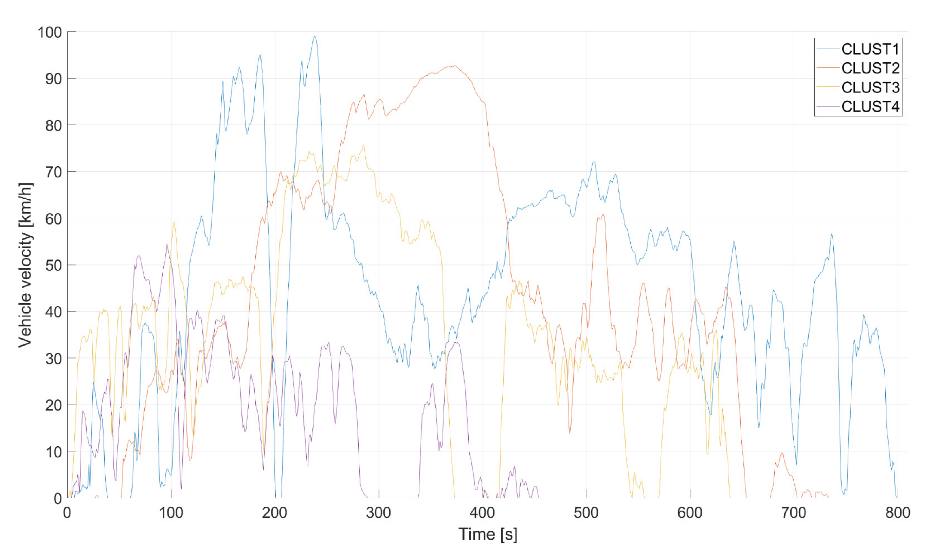
  • The identification of a test set of for the interpretation of the results obtained with the RL agent.
Once the theoretical framework has been discussed, the main results obtained when modifications are applied to the configuration of the Q-learning agent when tested on multiple experimentally derived DMs are reported. The main outcomes of the study can hence be resumed in what follows:
  • The assessment of the effect produced by a modification of the discount factor on its capability of defining an admissible control policy for different DMs;
  • The identification of the best fitting discount factor in case of a reward function focused on battery SoC sustaining as well as FC minimization;
  • The assessment of the combined effect produced by changing the reward function along with the discount factor;
  • The assessment of the effect produced by a change in the value of the learning rate;
  • The demonstration of the RL agent response to a change in the exploration strategy.
The paper is organized in such a way that RL for HEVs is introduced, recalling the fundamentals of mathematical formulation and the Q-learning specific algorithmic structure, then the software framework developed for the purpose of the present research is presented and, finally, the results of the entire study are presented.

2. Reinforcement Learning for Hybrid Electric Vehicles

Optimizing the energy management of a (P)HEV under real-time driving conditions is considered as one of the highest barriers to be overcome if consistent reductions in the overall emissions are targeted. In fact, the driving environment can change continuously throughout a given mission according to changes in the traffic, road conditions, weather conditions, driving behavior, etc. Moreover, FHEV and PHEV architectures are typically subject to different control policies due to the substantial differences in the powertrain. Therefore, the definition of an optimal control strategy in such a variable scenario can become a very complicated problem to deal with and several assumptions have to frequently be included in the analysis.
The general formulation of the problem accounts for an objective function J to be optimized under a control policy π and a set of boundary conditions. Within this paper, the problem to be solved refers to the minimization of the fuel consumption while achieving charge-sustaining (CS) of the battery.
According to [25], the mathematical formulation for the control problem of the FHEV considered in this paper can be represented by:
π * = min π f   J = min π f 0 T m ˙ f with   S o C T = S o C 0 V v t = V r t   for   t = 1 , 2 , , T
where π * is the optimal control policy (i.e., one control policy π among the feasible control policies f with the capability of minimizing the function J), m ˙ f is the actual FC, T is the final time step of the DM, S o C 0 and S o C T are the battery SoCs at the initial and terminal time steps of the DM, respectively, and V v t and V r t are the vehicle velocity and the DM velocity request at t-th time step, respectively. The FC minimization of the FHEV has hence been targeted including two boundary conditions: battery CS and compliance of the vehicle velocity with respect to the DM velocity request. As far as the battery charge level is concerned, the control problem has been set up considering that a charge-depleting strategy (i.e., S o C T < S o C 0 ) would need to refill the amount of charge (i.e., energy) in the battery during future DMs. Such a condition would lead to an additional future fuel consumption related to the charge depleting of the first DM. To this end, recalling that FHEVs do not include a battery recharge from the grid, a reliable comparison of the energetic performance realized by several FHEV architectures can be produced under CS conditions. As a second constraint, bounding the vehicle velocity to the velocity request of the DM ensures the control agent to learn action chains that could not drive the vehicle to higher or lower velocities with respect to the reference trajectory. Such an approach can be defined as “backward-facing”, because the driver response to a velocity input is not modeled, whereas a reference velocity has to be followed starting from the wheels and moving backwardly to the power and energy components.
According to the literature about optimization of HEV control, DP has proved to be capable of solving complex control problems under off-line conditions [26,27,28]. Thanks to the knowledge of the entire velocity trajectory throughout a given mission, the DP can be used to identify the optimal control policy in a completely discretized environment. Nevertheless, two main drawbacks are typically addressed by this approach when real-world conditions are considered [29]:
  • The entire trajectory of the vehicle velocity is not a priori known under real-time conditions;
  • The DP mesh discretization level could be too fine for the on-board electronics to solve a control problem under real-world unpredictable driving scenarios, i.e., the DP cannot be implemented in the electronic control unit (ECU) under real-time conditions.
Evolving from DP to RL could potentially represent a solution to these two problems. In the following sections, an insightful discussion about the possibilities of RL is presented. Moreover, the results of specific experiments are presented, aimed at thoroughly analyzing the behavior of RL under different training and testing conditions.

2.1. From Dynamic Programming to Reinforcement Learning

Among ML decision-making techniques, RL represents the family of algorithms featured by an agent interacting with an environment to reach a desired goal [16]. A feedback signal named “reward” is passed to the agent at each time step of a training episode as an index of the effectiveness of the action taken.
The agent–environment interaction can be formalized through a Markov decision process (MDP). A classic formulation of an MDP is completely described by a tuple < S ˇ , A ˇ , r, P, γ > where S ˇ is the state space (i.e., set of states); A ˇ is the action space (i.e., set of control actions available to the agent); r: S ˇ × A ˇ R is the reward function; P: S ˇ × S ˇ × A ˇ → [0, 1] is the state-action transition probability function; γ is the discount factor, a scalar value which expresses the agent’s preference of gaining a future reward with respect to an immediate reward. Moreover, consistent with the experiments presented in the following sections, a further assumption of S ˇ and A ˇ being finite (and discrete) can be made.
The RL workflow can be easily explained starting from the MDP tuple. At each time step t , the agent receives a set of information about the current state of the environment, denoted as s t . According to its control policy π , the agent chooses an action a t . In response to the selected action a t , the environment evolves its state from s t into s t + 1 based on the transition probability P. The reward feedback signal r t is hence released. An iteration of the learning procedure is then summarized by the tuple < s t , a t , r t , s t + 1 >. Once the procedure for a time step is completed, the system moves to the following time step t + 1 and the operations are repeated iteratively until a terminal state is reached:
e T = s 0 , a 0 , r 0 , s 1 , a 1 , r 1 , , s T 1 , a T 1 , r T 1 ,   s T
where e represents the trajectory of the agent–environment interactions within an episode while T represents the terminal time step. The training process can hence be satisfied by completing multiple episodes.
The MDP formalism requires the states to satisfy the Markovian property: the transition from s t to s t + 1 depends only on s t and a t and not on the complete trajectory from s 0 to s t [16]. Therefore, the transition probability function depends only on s t , a , s t + 1 :
P S t + 1 = s t + 1   |   S t = s t , A t = a t = P S t + 1 = s   |   S t = s t ,   ,   S 0 = s 0 ,   A t = a t
Both DP and RL are iterative solutions of the Bellman optimality equation [16]. The main difference between the DP optimization and RL lies in the knowledge of the transition probability function P. DP assumes the knowledge of P, so a direct solution of the optimal policy can be obtained offline, without interacting with the environment. Instead, no a priori knowledge about the environment is assumed in RL; therefore, the P function is neglected from the optimization.
As a final comment from an engineering perspective, the agent cannot always observe the entire state of the system as a significant number of signals might not be available during real-world conditions. Considering the problem of HEVs real-time control, the sensory input provided to the agent could not constitute the complete view of the environment (i.e., vehicle conditions, actual and future traffic, driver behavior, weather, etc.). In these cases, the agent–environment interactions cannot be modeled through Equation (2) and a distinction between state and “observation” needs to be introduced. The state s t , which satisfies the Markovian property of Equation (2), collects all the signals that represents the environment, whereas the observation o t is a subset of s t constituted by the set of signals which can be passed to the agent [16]. In other words, the observation should be designed to best approximate the Markovian property about the system state. Even though a theory about Partially Observable MDP [30] has been developed in literature which accounts for the violation of the Markov property for o t , the assumption of this paper is that o t satisfies the Markovian property.

2.2. Discounted Return and Discount Factor

The objective function of an RL agent is stated in terms of the “discounted return” G t at each time step [16]:
G t = R t + γ R t + 1 + γ 2 R t + 2 + = k = 0 γ k R t + k
In which γ ϵ [0, 1]. If γ = 0 leads the agent to a single-step optimization, γ = 1 involves the optimization of all the episode’s steps. In other words, lower γ push the agent to prefer an immediate reward, whereas higher γ would significantly increase the complexity of the problem faced by the agent. The choice of gamma determines the optimization horizon. A thorough discussion of the performance of an RL-based EMS for HEVs considering different discount factors is not typically made in the literature. As examples, no details about the value of the discount factor are provided to the reader in [20,21,22,23,24], whereas γ = 0.6 is selected in [22], apparently without a precise motivation. So, to close this gap, the response of the RL agent to different discount factors is discussed in the following sections by means of a specific test plan.

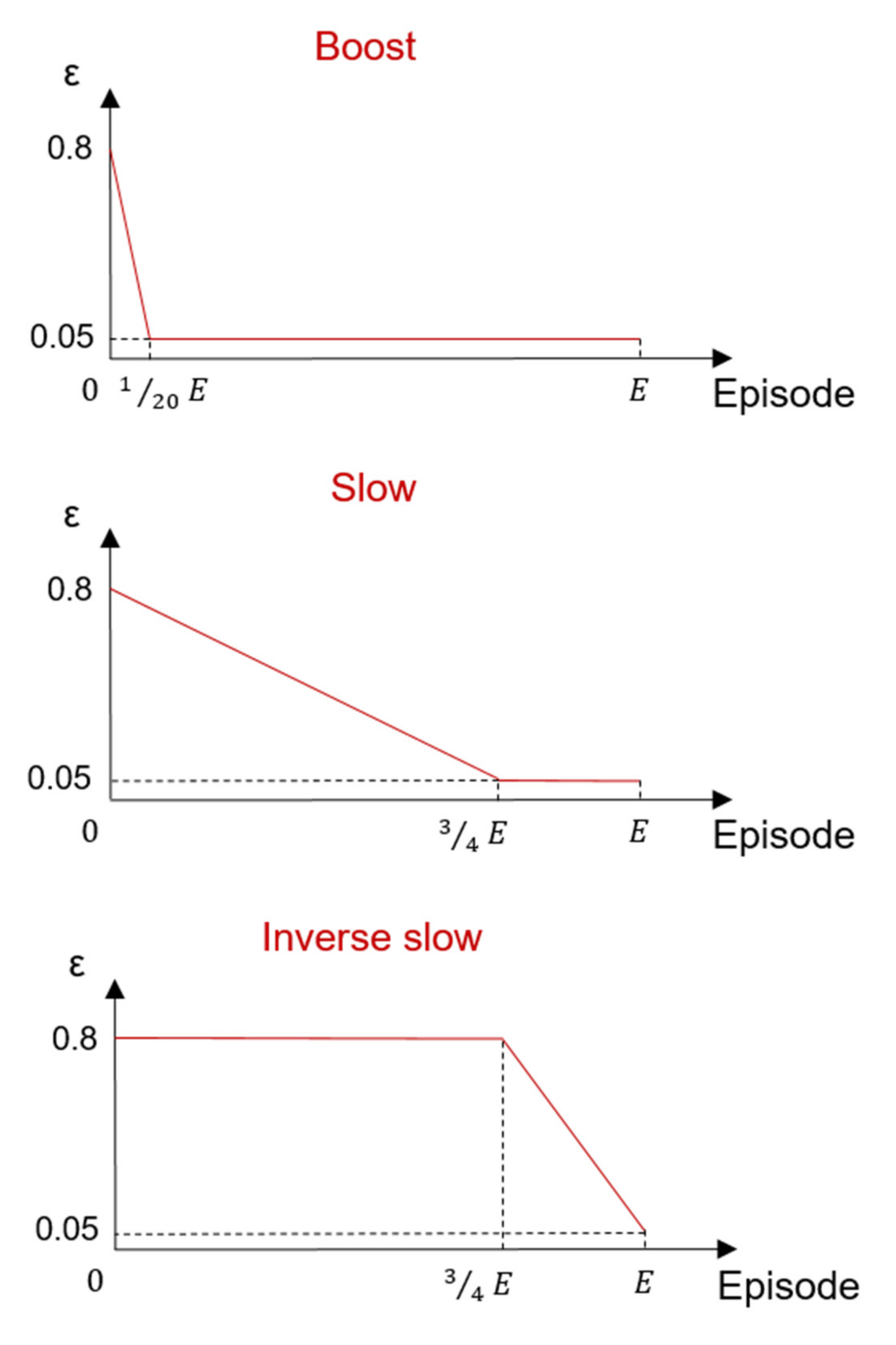
2.3. Exploration–Exploitation

No a priori knowledge about the environment is possessed by the RL agent. A critical challenge of RL is hence referred to as the trade-off between exploration and exploitation (“exploration-exploitation dilemma”) [16]. Exploitation refers to the agent’s decision of selecting the most effective action in a specific time step. Exploration is instead the condition of the agent to choose a random action among the set of feasible actions.
In the initial phases of the training process, the agent is typically asked to explore the environment and make experience. When the agent has acquired some knowledge about the environment, a trade-off between exploration and exploitation is imposed. In fact, the agent has to be pushed to define new ways to avoid being stuck in control strategies possibly conducting to local optima. One common solution refers to the usage of a “ε-greedy” method [16]. Consistent with this method, the agent mainly acts greedily (i.e., exploitation is way preferred to exploration) but maintains a small probability ε to select a random action.
The choice of the exploration strategy could be crucial on the RL-based EMS for HEV decision process. In the present paper, three different exploration laws have been employed and are charted in Figure 1 with respect to the training episodes. The speed of the exploration rate ε falling from a high initial value (0.8) to a very low final value (0.05) has been considered to properly label the exploration strategy. Specifically, the agent is allowed to explore the environment with a progressively decaying probability of selecting a random action in the first 5% and 75% of the training episodes in “boost” and “slow”. On the contrary, a fixed exploration rate until 75% of the training process followed by an increasing percentage of exploitation is considered in the “inverse slow” strategy.
The exploration component of the RL policy can mislead the evaluation of the actual performance of an RL algorithm. This is caused by the stochasticity of the exploration which causes the agent to modify the action to be applied. Therefore, the proposed methodology for an exhaustive project of an RL agent for HEVs distinguishes between training and testing episodes. During training episodes, the agent is allowed to use the exploration strategy to collect the transition useful to gain more information about the environment. Instead, during testing episodes, the exploration is not permitted, and the agent can only choose greedy actions within the episode.
This said, two final considerations can be made about testing episodes. First, at the end of the training process, a testing episode has to be performed to check on the real performances of the trained RL agent. Second, despite the difference in the exploration strategy, the agent could be tested with a user-defined frequency so as to track the learning progress of the agent. In the following sections, the usage of testing episodes will be presented both for in-training and out-of-training phases.

2.4. Reward Function and Shaping

The effectiveness of a generic action taken by the agent can be expressed by means of the reward feedback signal. The identification of a proper definition for the reward function has to be made based upon the specific case study. In the present paper, the problem of minimizing the FC of a HEV under real-time conditions is targeted considering two boundary conditions, namely battery CS and compliance with the DM velocity profile. Within this framework, three different reward functions have been identified. The number and typology of variables included in the reward functions have been defined considering the HEV control problem and the necessity of producing different reward orientations. The reward functions have been expressed as:
R = R 1 = k 1 + k 2 · S o C S o C * 2 + k 3 · F C R 2 = k 1 + k 3 · F C + k 4 · F C e q T R 3 = k 1 + k 3 · F C + k 5 · F C e q
In which k 1 5 are numerical coefficients to be tuned, S o C * is a reference battery SoC value, S o C is the actual battery SoC value and F C e q is the equivalent FC calculated as:
F C e q = S o C S o C * · E b , w H i · η ¯ I C E
where E b , w is the battery energy content related to the admitted battery SoC window, H i is the lower heating value of the fuel considered for the specific ICE application and η ¯ I C E is a fixed average ICE efficiency value. Consistent with the World harmonized Lightduty Test Procedure (WLTP), the equivalent FC has been calculated only in case of S o C < S o C * . In (5), the difference between F C e q T and F C e q is that F C e q T is calculated only at the final time step T , whereas F C e q is calculated at each time step (in case of S o C < S o C * ).
For the sake of clarity, R1 is a battery SoC-oriented reward function, whereas R2 and R3 are progressively more FC oriented. To this end, the coefficients k 1 5 have been tuned so as to satisfy these assumptions made for the reward functions. Additional parameters as well as a procedure for the fine-tuning of the numerical coefficients could be considered for the optimization of the reward functions. Nevertheless, the aim of the present paper is to present and discuss a complete project of RL along with an exhaustive test plan for the problem of HEVs control. The research of the optimal performances obtained for a specific HEV application is beyond the scope of the paper. Therefore, the selection of the different reward functions presented in (5) has been considered as a reliable step for the assessment of the response generated by the RL-based EMS under very different conditions even without research of the optimal results. Considering the three different reward functions of (5), a reward shaping analysis is presented for HEVs in the following sections.

2.5. Q-Learning Algorithm

The core part of the RL agent is constituted by the algorithmic structure as well as by the transition (step) function used to stimulate the learning process. The Q-learning algorithm is one of the first and most studied RL algorithms proposed in the literature [31]. It is based on the idea of the maximization of a q-value q π ( s | a ) . The estimate of the optimal q-value is obtained iteratively by means of the Temporal Difference (TD) principle that provides updates for every time step using the received reward [16]. The idea of the Temporal Difference (TD) method is based on the TD-Target: R t + 1 + γ Q S t + 1 ,   A t + 1 which represents a slightly better approximation of the q-value for each of the state-action pairs. For each time step, the TD algorithm updates the approximation of the q-value in the direction of the TD-Target. The update is computed by the minimization of the TD-Error, which is represented by the difference between the new estimate and the old one: TD-Target Q S t ,   A t . The entity of the update is controlled by the learning rate α .
The mathematical formulation for the TD-update is:
Q s t ,   a t Q s t , a t + α R t + 1 + γ Q s t + 1 ,   a t + 1 Q s t ,   a t
Starting from the TD update, Q-learning computes the target of the q-value approximation computing the estimation max q-value starting from the state of the next time step s t + 1 , where the max is computed among the action available to the agent at time step t . In other words, the q-value estimates involve the choice of the greedy action on the next state, that is, an estimate of q * . In the Q-learning algorithm, the mathematical formulation becomes:
Q s t ,   a t Q s t , a t + α R t + 1 + γ   m a x a A ( s t + 1 ) Q s t + 1 ,   a Q s t ,   a t
In addition, the Q-learning stores the q-value estimate for each state–action pair in a matrix named Q-table. Given a state s t , the Q-table gives the priority over the choice of the actions at time step t , the greedy action being the one with greatest q-value a r g m a x a   A s t   Q ( s t ,   a ). The policy π of the Q-learning agent is the ε-greedy policy with respect to the q-values of the state s t . Considering that not the entire set of actions could be available to the agent at each time step in a real driving scenario, some actions are known to be unfeasible in a state s t ; therefore, they can be excluded from the actions among which are computing the q-values, both for the update and for the policy π . In particular, the set of actions A ( s t ) among which the agent can choose at time-step t depends on the state s t of the environment at the same time step.

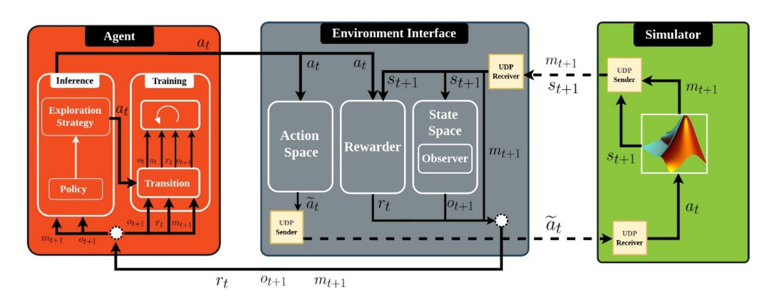
3. An Integrated Modular Software Framework for Hybrid Electric Vehicles

This paper proposes a testbed to design an RL-based control strategy for a passenger car HEV. The implementation of the proposed testbed has required the development of a software platform. In this section, an integrated modular software framework (IMSF) used to conduct extensive and reproducible experiments for the design of a RL-based control strategy evaluation is described. The IMSF is compatible with the OpenAI gym Python library [32].
The tool realized to produce such results is characterized by four distinct elements: a Simulator, an Environment, a Communication Interface and an Agent. The elements composing the complete software framework are illustrated in Figure 2. The framework is designed to be general purpose and modular. The modules of the Agent and of the Environment are written using the Python 3.8.5 programming language [33]. The HEV simulator is written using MATLAB®. The Communication Interface allows the exchange of information between the Simulator and the Environment by means of the UDP communication protocol, written in MATLAB and in Python. The IMSF is designed to be complete and general, that is, to manage the training of any RL Agent in every simulated Environment. Each module is thoroughly described in the following sections. For the IMSF, the reproducibility is guaranteed by complete configurable modules. The configuration of each experiment can be stored in a separated database to reproduce the obtained results. The modularity is guaranteed by having the interfaces being the same for all the module instances, e.g., all the possible agents, simulators, reward function and so on.

3.1. Simulator

The pre-transmission parallel HEV architecture reported in Figure 3 has been modeled and employed as a Simulator of the software framework. The layout refers to the driveline of a hybridized front-wheels driven passenger car equipped with a conventional downsized ICE and a 6-gears transmission. A kinematic backward approach has been used to compute the power requested to the different stages of the powertrain (from wheels to the power components) according to [34,35,36]. The final drive (FD) and the torque coupling device (TCD) have been modeled as fixed speed ratios; clutches have been included in the powertrain to allow the HEV for exploiting its macro-operating modes during traction conditions. Specifically, a pure thermal mode can be realized by engaging the clutch C1 while disengaging the clutch C2 so that the ICE can be used as a stand-alone component. A pure electric mode can be realized by engaging clutch C2 while disengaging clutch C2 so that the MG (and the battery) can be used as a stand-alone component. A power-split mode can be realized by engaging both clutches C1 and C2 and demanding power to both the propellers. Finally, a battery charging mode can be obtained by engaging both clutches C1 and C2 while using the MG as generator with the capability of transferring a given share of power to the battery even during traction. Evidently, the ICE is demanded to produce a higher power with respect to the power requested by the road. Efficiencies have been considered for each powertrain component, including FD, multi-gears transmission (TR), torque-coupling device (TCD) and AC/DC converter. Each of these, except TR, has been simply modeled as a fixed efficiency to be paid both during traction and braking phases. About TR, a different efficiency has been considered for each gear. Moreover, experimentally derived two-dimensional look-up tables have been used to estimate the fuel consumption and the motor efficiency of the ICE and the MG, respectively. Finally, the battery performances have been accounted for by a fast-running low-throughput Rint model in which the effect of environmental temperature, battery temperature and aging process have been ignored [29]. For the sake of clarity, moving to a more detailed battery model would have led to a relevant increase in the computational time needed by the software calculations while not changing the focus of the present study. In fact, even with a change in the numerical results obtained by the RL control algorithm, any step would have changed in the approach. Extending the study of the RL performance when coupled with detailed physical models will be considered a future step.
The Simulator receives the Agent’s physical action a t ˜ for the current time step (please refer to next section for the definition of physical action) and it generates the new state s t + 1 . During this process, it also produces the action feasibility mask m t + 1 , which represents the set of actions allowed to the Agent at each time step t . Assuming a discrete action space, the action feasibility mask can be represented as a boolean vector that excludes from the action space the actions physically impossible from the state just generated. The feasible actions have been represented by 1 whereas unfeasible actions have been represented by 0. The latter could be obtained based on two specific conditions: the power requested by the road is not realizable or the battery SoC window has been exceeded.

3.2. Environment Component

The Environment is a module that works as a bridge between the Agent and the Simulator. It has been built based on the OpenAI gym standard. Three main submodules highlight: Action Space (AS), State Space (SS) and Rewarder (REW). Each of them is hereafter detailed.
AS represents the module responsible for handling the action proposed by the Agent and hence executed in the Simulator. Physical and logical action can be distinguished, a t ˜ and a t , respectively. The physical action a t ˜ is the actual action applied to the HEV powertrain according to the control policy in a single time step. In the present research, the operating mode of the HEV (i.e., pure thermal, pure electric, power-split or battery charging) as well as the gear inserted in the transmission have been considered as the set of plausible physical actions. The logical action a t is a logical representation of the physical action a t ˜ for the Agent. In the Environment, the AS submodule is hence devoted to map the physical action a t ˜ into the logical one a t and send the feasibility mask m t received from the Simulator to the Agent. If needed, the AS can also handle both discrete and continuous actions.
The second submodule is the SS. As explained in Section 2.1, the Agent does not receive the full state as input but only an observation that contains partial information of the true state. SS is responsible for the conversion of a state s t produced by the simulator into an observation o t for the Agent. The process that leads to the generation of the observation is divided into two main steps. An Observer is first asked to filter the state to maintain only the realistically available information in a real-life context. Then, the Agent can receive the observation in a discrete or continuous space. If in the discrete space, the filtered state is further processed by means of a discretization; otherwise, if in continuous space, the filtered state is standardized to a [0, 1] range.
The third submodule is REW, which is responsible for computing the reward r t based on the couple of state and action. The calculated reward r t is hence sent to the Agent as feedback for the taken action a t .

3.3. Agent Component

The last module of the IMSF is represented by the Agent, which is responsible for identifying the optimal policy π * . The Agent is hence capable of choosing the logical action a t for every received observation o t based on the specific exploration–exploitation trade-off explained in Section 2.3. As for the Environment, three submodules are included in the Agent: Policy, Exploration Strategy and the Training.
The Policy submodule is devoted to calculating the selection priority of each logical action available at a given time step.
The result of Policy is sent to Exploration Strategy that is asked to output the exploration rate given a specific exploration strategy. At each time step, it takes the Policy priority values as inputs along with the action feasibility mask m t and it outputs a choice between the feasible actions according to the priority. In particular, if the exploration strategy is the greedy strategy, the action chosen would result in the one among the feasible actions having the maximum priority.
Finally, the Training submodule collects a transition and updates the internal decision model of the Agent according to a specific algorithm. During the training episodes, the Agent chooses the action according to the chosen exploration and updates the internal decision model. During the testing episodes, Exploration Strategy chooses the greedy action according to the feasibility mask and no update of the decision model is made.

3.4. Communication Interface
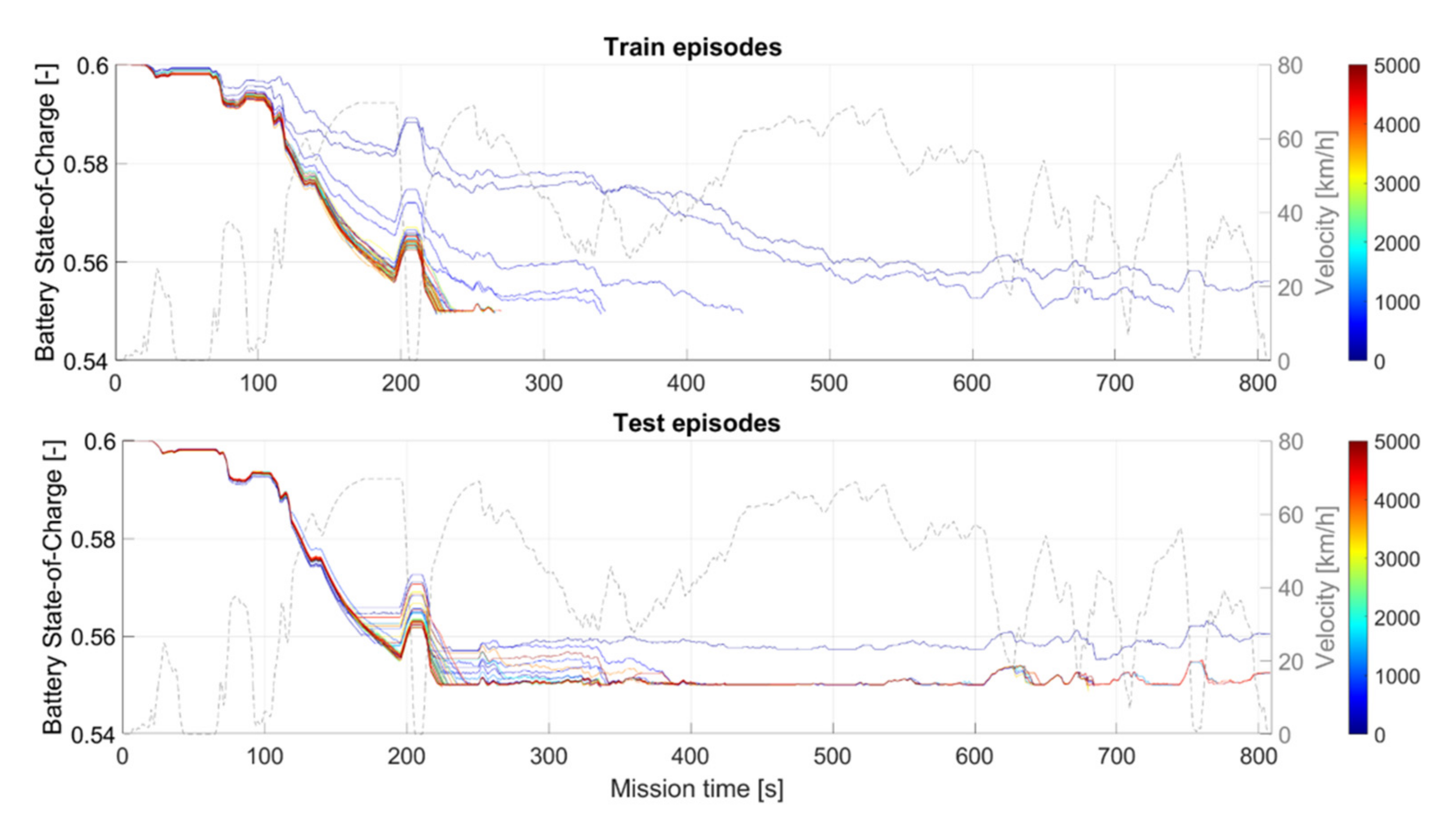
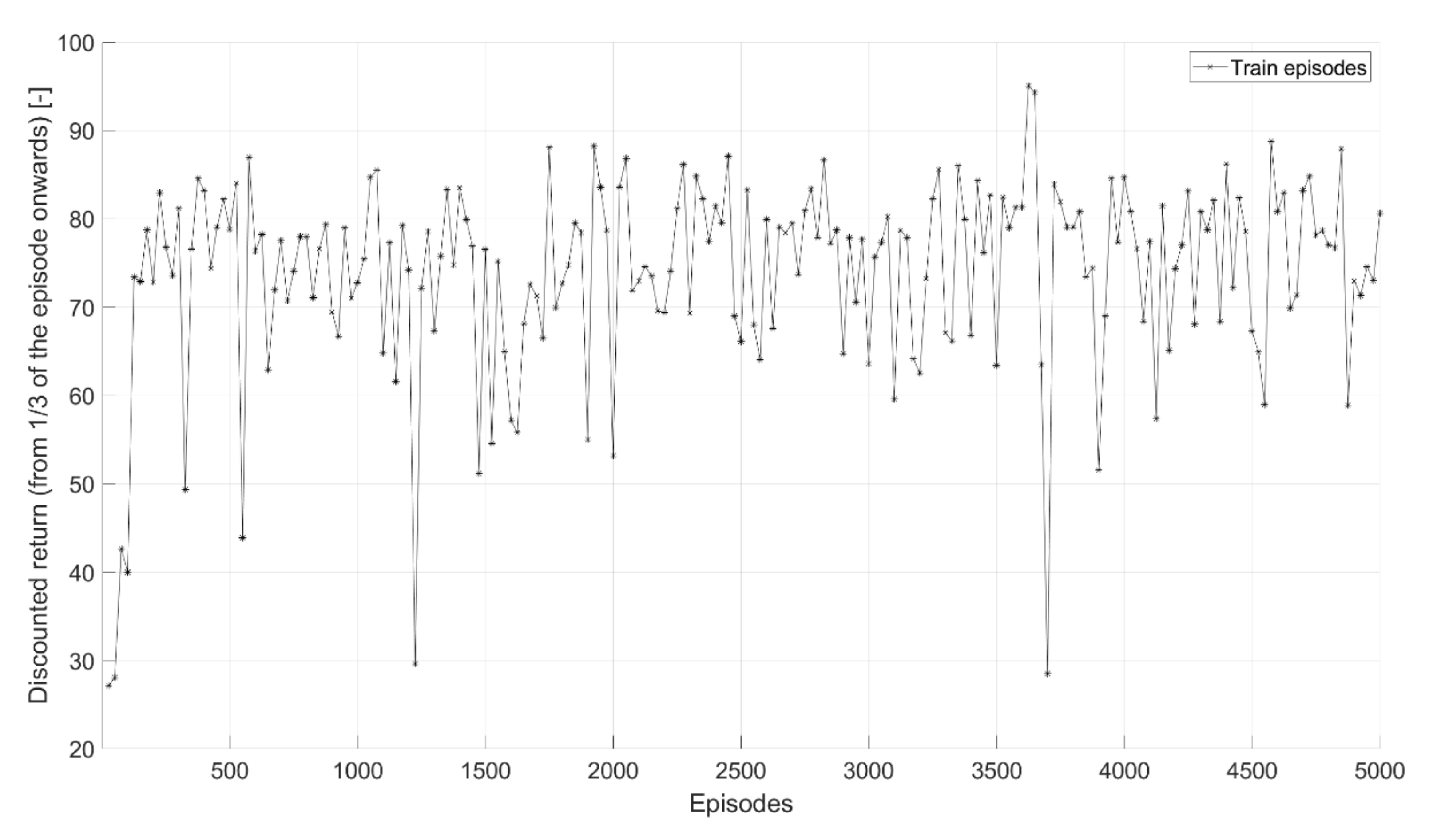
The communication interface module allows the co-simulation between two different parts of IMSF that are written in different programming languages. In our framework, the communication interface allows the synchronization between the Environment written in Python and the simulator written in MATLAB. The synchronization between the two processes is realized through a message-passing system built over a UDP communication protocol in a local network.
In order to communicate through the UDP protocol, at each step, all the data are collected, stacked into a list, and encoded into bytes format before being sent. The same process, in reverse order, is computed when the data are received.

4. Results

The design of a RL-based agent for the control of HEVs requires the analysis of a set of meaningful experiments aimed at assessing the change in the performance of the algorithm when consistent changes are applied to its configuration. Therefore, the identification of an exhaustive test plan of the agent has to be carried out. In the present section, the results obtained by a thorough analysis of the Q-learning response when used as control agent for a HEV are analyzed relating to the variation of the most influencing parameters defined in Section 2.
The main characteristics of the considered parallel HEV (Figure 3) are listed in Table 1. The conventional driveline has been integrated with a 70 kW MG and a 74 kW–6.1 kWh battery. The peak power of the MG has been considered both for traction and regenerative braking phases since a symmetrical operating map has been involved in the analyses. About the energy storage system, a sizing operation has been performed so that the peak power achieved by the battery could fulfill the power requirements of the MG, both during traction and regenerative braking conditions.
The HEV performances have been evaluated on four different experimentally derived DMs [37], identified as CLUST1, CLUST2, CLUST3 and CLUST4.
In Figure 4, Figure 5, Figure 6 and Figure 7, some of the main characteristics of each DM are compared, specifically the vehicle velocity as a function of time, the vehicle as a function of distance traveled, maximum vehicle acceleration and velocity and average vehicle acceleration and velocity. The selection of the DMs has been based upon the necessity of testing the RL control agent for HEVs in a driving environment characterized by a miscellaneous set of driving conditions. As far as the vehicle velocity profiles are concerned, the longest DM among the four is CLUST1, whereas CLUST2, CLUST3 and CLUST4 are progressively shorter. Moreover, CLUST1 is featured by the highest maximum and average velocities. On the contrary, the shortest DM (CLUST4) involves the most demanding average acceleration during traction, as it can be seen from the very spiky velocity trajectory charted in Figure 5. The maximum acceleration during traction is achieved on CLUST3, whereas the less demanding operations are required on CLUST2.
So as to provide a fair comparison between the performances of the different tested Q-learning configurations, the results obtained by the DP on the same environment have been considered as benchmark in the case of S o C * = 0.6. Moreover, the state and control variables of the DP have been identified based on the observations and the actions of the Q-learning agent (i.e., battery SoC as observation, power flow and gear number as actions), respectively. As for the battery SoC discretization, the same mesh has been applied to the DP computational grid as well as to the Q-table of the Q-learning algorithm according to [29]. Specifically for the present case of study, 501 levels have been considered in a battery SoC window of [0.55–0.65]. As far as the control space is concerned, the set of Q-learning actions has been paired to the set of DP control variables. Specifically, two indexes have been considered for the gear number (GN) and the power flow (PF), resulting in 42 possible actions (6 gears and 7 possible power-splits between ICE and MG). Finally, the objective function of the DP has been set according to the problem formulation of (1), for which the FC has to be minimized while a complete battery charge sustaining (CS) is attained. For the sake of clarity, no optimization of the Q-learning agent for the specific vehicular application is targeted in this study. The results of the Q-learning presented in the following section have hence not been considered as representative of the best performances that could be obtained by an optimized Q-learning version.
According to the main hyper-parameters discussed in Section 2, the results shown in the following sections will mainly focus on:
  • Effect of γ;
  • Reward shaping;
  • Sensitivity to α;
  • Variation of the exploration strategy.
Other parameters have not been included in the test plan since an easier tuning operation could be identified, such as the maximum number of episodes in the experiment. As an example, if any limitation would have existed about computational time, a very large number of episodes could have been set so as to be confident about the possibility of the agent to converge to its best performance. The performance of the algorithm is assessed by means of the battery SoC trajectories realized during and at the end of the training and testing processes, the cumulative fuel consumption, the real fuel consumption and the shape of the discounted return.

4.1. Effect of γ

The performance of the Q-learning agent for the control of a parallel HEV on CLUST1 has been assessed for studying the influence of the value considered for the discount factor. Recalling Section 2.2, reducing the value of the discount factor leads the agent to favor actions based on an immediate reward, whereas future rewards can be accounted only by increasing the value of γ. The real-time control of HEVs requires a balance between the battery SoC CS around S o C * and FC minimization. Therefore, an agent preferring actions based on immediate rewards might not lead to robust solutions. As an extreme experiment, a null value could be assumed to demonstrate an expected inefficient setup of the agent. On the contrary, the value of the discount factor could be increased toward one, predicting better agent performances.
Regarding the whole agent configuration for the analysis over the effect of γ, reward function R1, α = 0.9 and boost exploration strategy have been considered. Moreover, a CS strategy has been considered only when a final battery SoC equal to 60 ± 2.5% (0.6 ± 0.025) is achieved at the end of the DM. Consistently, the final fuel consumed at the end of the DM has been considered only for the experiments featured by battery CS trajectories. In fact, since the final fuel consumption is calculated relying on the estimation of an equivalent fuel consumption (6), the accuracy of the estimation of the equivalent fuel consumption can play a significant role in the results. Therefore, a minimization of the impact of inaccurate estimations of the equivalent fuel consumption is to be pursued. Such an event is clearly obtained when a complete CS trajectory is achieved. On the contrary, if a CS trajectory is not obtained, introducing a threshold in the maximum and minimum battery SoCs could allow for excluding unrealistic calculations of the final fuel consumption.
The discounted return evaluated at the first time step of the CLUST1 is reported in Figure 8 in case of γ = 0. Neglecting the role of γ in (8) leads to the generation of a constant discounted return. The agent is pushed to learn a control policy only based on the actual reward, without accounting for the implication of the chosen action in the future. In Figure 9, the trends of the battery SoC are charted both for training (top chart) and testing (bottom chart) episodes for the first and last episodes of training and testing, respectively. As it can be clearly noted, the agent is not capable of sustaining the battery SoC during the training process, which turns into an unsatisfying result for the testing process. According to such a bad utilization of the electric path, the cumulative fuel consumption does not represent an interesting result and it is hence not considered. The results obtained by applying the same Q-learning configuration for CLUST2, CLUST3 and CLUST4 have shown the same behavior and, therefore, they are not reported for briefness.
Differently from the case of γ = 0, increasing the value of the discount factor enhances the influence of the outcome of future time steps on the agent’s decisional process (Section 2.2). The change in the performance of a Q-learning controller for HEVs has hence been assessed for higher discount factors. Specifically, the discount factor has been set to 0.9, 0.99 and 0.999. In Table 2, the results obtained when a variation of γ is introduced in the agent configuration are reported for each DM. The final battery SoC ( S o C f ) always falls within the CS window except for the case of γ = 0.999 on CLUST3. The latter represents a hard environment to be solved by the algorithm as it is characterized by a short but spiky velocity profile with strong accelerations and decelerations. Consistently, the entire set of actions is not feasible during multiple time steps of the DM. Such conditions can significantly reduce the number of control trajectories to be explored during the training process, affecting the capability of the agent to define robust control policies. For the sake of clarity, an optimization of the Q-learning configuration should have been carried out to provide the control agent with the optimal settings to properly solve the control problem over CLUST3. Nevertheless, discovering unsolved problems is a coherent result with respect to the aim of the present paper. Significant differences arise in the absolute values of both fuel consumption (FC) and real fuel consumption (rFC) achieved with the different γ configurations. The different between FC and rFC consists of an additional FC included at the end of the experiment if S o C T < S o C * .
In other words, rFC is equal to the sum of the FC at the end of the mission and the equivalent fuel consumption F C e q related to the difference in the final battery SoC. In fact, given the different durations and lengths of the four DMs, a very different cumulative FC can be expected at the end of the experiments. Specifically, CLUST1 and CLUST2 are longer DMs and highlight larger fuel utilization, and vice versa for CLUST3 and CLUST4. A lower γ value (0.9) appears to outperform higher values for each driving environment in terms of rFC. On the contrary, a clear trend is not introduced by increasing γ to 0.99 or 0.999 but different behaviors can be obtained for the different DMs. Specifically, the intermediate value (0.99) outperforms higher values only on CLUST2 and CLUST3, whereas the highest tested value leads to a better result on CLUST1 and CLUST4. According to this non-trivial response of the Q-learning, testing the RL agent with multiple values of the discount factor appears to be a fundamental step when the identification of a specific reward function has been made.
The most interesting trends related to the best experiment over CLUST1 (γ = 0.9) are reported in the next charts. The training discounted return evaluated at initial time step, 1/3 and 2/3 of CLUST1 are shown for the entire experiment in Figure 10, Figure 11 and Figure 12, respectively. Differently from the result obtained with a null discount factor, different values can be obtained throughout the experiment. Specifically, the discounted return appears to converge right after the first episodes (90.675) when calculated in the first time step of the driving mission, whereas a larger number of episodes is necessary for the discounted return to reach a stabilization farther in the driving mission. In fact, the discounted return of Figure 11 reaches starts from a very low value (~27), and it requires ~500 episodes to encounter a kind of stabilization; furthermore, a negative discounted return occurs at the beginning of the experiment and ~500 episodes are needed to converge at 2/3 of the mission (Figure 12). As an outcome of this study, the agent appears to be capable of learning the optimal decisions to be taken throughout the entire driving mission. Such a set of results based on the discounted return is fundamental if realistic information about the learning progress of the agent is to be gained. In fact, evaluating the discounted return in a single step of the driving mission does not provide the user with an exhaustive outcome about the capability of the RL agent to select the best actions during the entire mission.
Other meaningful trajectories for the problem of HEVs real-time control are represented by the battery SoC and the cumulative FC realized by the RL agent over the driving mission. In Figure 13 and Figure 14, the trends of the battery SoC evaluated in one of the first and the last episodes over CLUST1 are charted both for training and testing conditions, respectively. Evidently, the agent proves the capability of realizing a CS battery SoC trajectory at the end of the experiment, whereas a very poor control policy is highlighted at the beginning of the experiment. An interesting outcome is also represented by the difference between training and testing episodes. In fact, the final battery SoC of the last testing episode (0.5838) is closer to the reference value (0.6) with respect to the one obtained in the last training episode (0.5760). As far as the cumulative FC is concerned, Figure 15 and Figure 16 highlight the agent capability of maintaining roughly the same FC during training and testing, respectively. This can be considered a consistent result of the training process since the achievement of improved CS trajectories is not affecting the final FC.

4.2. Reward Shaping

Within this section, the results produced by a reward shaping analysis over the Q-learning agent are reported considering the three non-null values of discount factor considered in Table 2. The best performing combination of reward function and discount factor has been identified (and highlighted in grey) for each DM.
In Table 3, the results obtained on each DM for γ = 0.9 are reported considering the final battery SoC ( S o C f ), the measured fuel consumption (FC), the real fuel consumption (rFC) and the relative difference between the real fuel consumption produced by Q-learning and DP ( Δ F C ). As for the analysis about the effect of γ on the agent performance, reward R1, α = 0.9 and boost exploration strategy have been considered for the present analysis. The adoption of the lowest non-null value of γ shows very interesting results when matched with the reward function R1. The agent is capable of completing the experiments on each DM with final battery SoC values within the CS window (>0.58) and promising final fuel consumption with respect to DP for CLUST1. On the contrary, matching γ = 0.9 with R2 does not lead to a good response of the control agent. Regardless a change in the formulation of R2 (i.e., R2a, R2b and R2c), the agent is never capable of exploiting a complete CS, hence invalidating the entire set of experiment. Finally, the results produced by adoption of the reward function R3 fall in between those obtained by R1 and R2. A CS trajectory is achieved for three out of four DMs, with final battery SoC nearer to the reference value (0.6) and real fuel consumptions comparable with those obtained by R1.
In Table 4 and Table 5, the same experiments have been carried out considering γ equal to 0.99 and 0.999, respectively. As it can be seen, the response of the agent when considering R2 is always negative. Indeed, matching R1 and R3 with higher γ values leads to different and interesting results with respect to γ = 0.9. First of all, the final battery SoCs are closer to the reference value for CLUST1, CLUST2 and CLUST4, which is a positive index about the agent capability of learning CS strategies. Second, no significant differences arise about the real fuel consumptions produced on CLUST1, CLUST2 and CLUST3 with respect to those obtained with γ = 0.9. Such a result can be read as the demonstration that consistent Q-learning behaviors can be obtained by using different couples of γ and reward function. Specifically, R1 proves to be more effective on CLUST1 and CLUST3 in case of γ = 0.99, whereas R3 is better for CLUST2 and CLUST4. For γ = 0.999, R3 can outperform R1 on CLUST3 while producing very similar results for CLUST2 and CLUST4.
Recalling Section 2.4, the reward function R1 is SoC oriented while R2 and R3 are FC oriented. Such a consideration is fundamental to justify the difficulty of the agent to solve the problem in case of R2 and R3. In fact, a more complex problem has to be faced when R2 and R3 are considered since a lower priority is given to the battery SoC trajectory. In this case, unfeasibility conditions related to the battery SoC exceeding the limits imposed by the battery SoC window are more likely to be exploited. Therefore, higher discount factors (i.e., larger time horizons for the discounted return) could be considered as they have proved to allow for stronger agents in cases of very complex problems.
Consistent with the results of the reward shaping analysis, a strong interaction between discounted return and reward function has been demonstrated. A non-trivial agent response can be obtained when reward functions with different levels of complexity are coupled with the discount factors and tested on different driving conditions.

4.3. Sensitivity to α

Another important factor to be analyzed when dealing with the assessment of the performance of a Q-learning algorithm is represented by the learning rate α. As for the discount factor, a sweep over three different values has been performed, specifically 0.1, 0.5 and 0.9. For the present analysis, the best combination between reward function and discount factor has been selected: R1 with γ = 0.9. The boost exploration strategy has also been maintained.
In Table 6, the results obtained by the control agent are reported for each DM. As for previous experiments, CLUST3 appears to be the hardest driving environment to be solved when moving from the original combination of R1, γ = 0.9 and α = 0.9. Moreover, unexpected results can be obtained on different DMs when drastically changing the agent configuration. As an example, a very low learning factor can be capable of outperforming even the most common values (e.g., 0.9) on specific DMs. Specifically, the lowest rFC is exploited by Q-learning with α = 0.1 on CLUST2 while a comparable rFC with respect to α = 0.9 is obtained on CLUST1. As far as α = 0.5 is concerned, such a configuration appears to be not optimal in minimizing the FC whereas it is capable of achieving the best CS results for CLUST1, CLUST2 and CLUST4.
Since the learning rate generally determines the speed of the Q-table update, a non-trivial response of the agent has been proved for throughout the present test cases. In fact, substantial variation can be obtained in the behavior of the agent when a reduction in the α value is introduced in the Q-learning setup. Nevertheless, as a general outcome of several research works in the literature, a higher value leads to more robust RL controllers for HEVs.

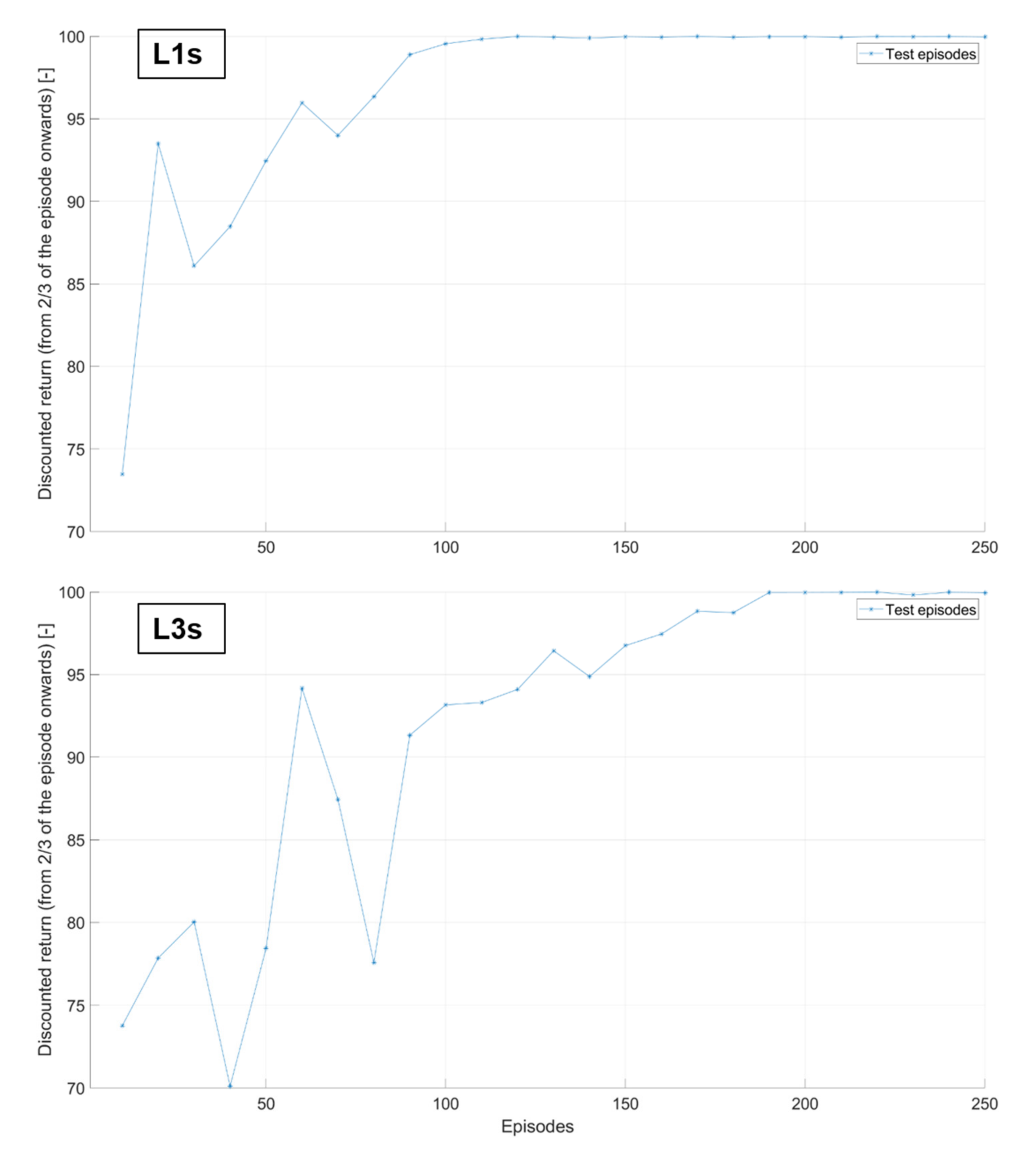
4.4. Variation of the Exploration Strategy

As a final step, the exploration strategy of the agent has been varied according to the strategies shown in Section 2.3. Any of the considered exploration strategies are featured by a linear decay of the exploration rate followed or preceded by a constant trace. Specifically, “boost” and “slow” are characterized by two decays with different slopes followed by a horizontal phase with ε = 0.05. On the contrary, a horizontal phase with ε = 0.8 is maintained for the majority of the experiment and then followed by the linear decrease in “inverse slow”. The three exploration strategies will be hereafter referred to as L1, L2 and L3, respectively.
Different from the results shown in the previous sections, a clear trend is highlighted by the results reported in Table 7 considering the entire set of DMs. In fact, L1 appears to be the best performing exploration strategy as it allows the agent to solve any environment (i.e., complete the missions) while minimizing the FC. L2 and L3 are capable of producing more accurate CS trajectories as the final battery SoCs are comparable with those obtained with DP. Nevertheless, the rFC values are worsened with respect to those achieved with L1. Moreover, the velocity trajectory of CLUST3 cannot be fulfilled as both L2 and L3 are not capable of completing the driving missions without falling outside of the battery SoC window (0.55–0.65).
Since L1 is characterized by a very short exploration boost with respect to L2 (and even more with respect to L3), an additional analysis has been performed by assessing for the learning process of the agent during the very first episodes of the experiment. For this purpose, L1 and L3 have been applied, considering very short experiments with “only” 250 episodes on CLUST1, namely L1s and L3s.
A comparison of the discounted returns evaluated at the first time step, 1/3 and 2/3 of the CLUST1 is reported in Figure 17, Figure 18 and Figure 19, respectively. Looking at trends of the discounted return at the beginning of the driving mission, no real difference arises when the exploration strategy is changed since an almost constant value is achieved throughout the entire episode. On the contrary, a significant difference occurs both at 1/3 and 2/3 of the driving mission when L3s replaces L1s. The larger number of episodes with ε > 0.05 creates a lag in the number of episodes needed by the discounted return to reach the convergence. Indeed, the stabilization is achieved faster when a shorter exploration boost is defined and a longer exploitation period is allowed to the agent.
As a confirmation of the trends highlighted by the discounted returns along the driving mission, the effectiveness of a specific RL agent for HEVs has to be confirmed through the results of S o C f and rFC. The latter are reported in Table 8 for both L1s and L3s. The results highlight that the agent is capable of reducing the rFC under L1s (with respect to L3s) even when a much shorter exploration boost is considered. The speed of convergence associated to the discounted return allows the agent for more robust performances. Nevertheless, considering the results of boost with larger experiments (Table 7), enlarging the constant ε region leads the agent toward a progressive adaptation of the final battery SoC in favor of a better rFC.

5. Discussion

The present paper aims at providing the reader with a comprehensive view of a thorough experimental test for a Q-learning algorithm to be implemented as HEV real-time capable EMS. The experiments conducted in the research activity are hence aimed at providing the reader with a complete procedure for a reliable assessment of the performance obtained by a RL algorithm for HEVs.
Two elements have been introduced to evaluate the agent performances. First, the distinction between training and testing episodes. Training episodes are featured by law about the agent exploration rate. On the contrary, the agent exploration strategy is turned off and the greedy action is always selected in testing episodes. Second, the identification of the discounted return during training and testing episodes as the most meaningful signal about the learning process of the RL agent. Contrarily, the sum of the rewards obtained by the agent in the episodes is typically used in the literature. Thanks to the present research, the trend of the discounted return computed in different time steps of training or testing episodes has proved to be a consistent index for the assessment of the RL agent performances.
In addition, the evaluation of the response of a Q-learning agent has been discussed considering a massive testing of the algorithm on different real-world driving conditions. Specifically, four different analyses have been conducted and thoroughly presented in this paper which are commonly neglected in the literature. First, the effect of the discount factor on the decisional process of the agent has been analyzed considering very different discount factors. Starting from the case of a null discount factor, an improved performance of the Q-learning has been appreciated in most of the cases when the discount factor has been set to values toward the unity. Such an outcome has been proved by means of the discounted return trajectory evaluated at three different stages of the episode. Second, a reward shaping analysis has been carried out considering an optimization of the cumulative fuel consumed at the end of the driving mission in presence of a boundary condition about the battery SoC charge sustaining. Such an analysis has been conducted considering different discount factors so as to highlight the non-trivial response of the agent when the training parameters are mixed and tested over different environments. As an outcome, the FC-oriented reward function has proved to be more efficient when higher discount factors are considered with respect to a reward focusing more on the battery SoC CS. This can be addressed to the nature of the HEV control problem. A FC-oriented control strategy can, in fact, fall into unfeasible policies with a high frequency due to the difficulty of maintaining the battery SoC under the admitted SoC window when any information (or information with small relevance) is provided to the agent about the influence of the battery SoC variations on the system. Third, the influence of the learning rate on the performance of the Q-learning agent. Recalling the learning rate to be responsible of the Q-table rate of update, the algorithm has proved to be very sensitive to the variation of its internal learning parameter. In fact, a worsened response of the agent can be obtained when a reduction in the learning rate value is applied. On the contrary, higher values can push the Q-learning algorithm to better performances as already proved in the literature about RL for HEVs. Finally, the role of the exploration strategy has been discussed as the last analysis. Three different exploration strategies have been considered, featured by three different exploration rate decays. The fastest decay followed by a large number of episodes with a very high exploitation rate have proved to outperform other strategies featured by longer exploration rate decays. Such an outcome has been discussed both for extended experiments (with thousands of episodes) and short experiments (with few hundreds of episodes). Despite the change in the experiment duration, the Q-learning agent has achieved a faster convergence of the discounted return evaluated at different stages of the driving mission when a small exploration boost has been considered.
The results presented in the paper can therefore be considered as a demonstration of the broadness and the depth of the tests to be conducted on a Q-learning agent when a reliable comprehension of a RL-based EMS for hybrid powertrains is targeted.

6. Conclusions

In the present paper, a complete project and development of a Q-learning based energy management system for the real-time control of hybrid electric vehicles has been presented. The results of the Reinforcement Learning agent have been discussed considering a pre-transmission hybrid powertrain and real-world driving conditions. First, the general framework of Reinforcement Learning has been presented and insights about the main parameters of the algorithm have been given to the reader. Then, the integrated modular software framework developed within the research activity has been shown together with the three main modules (agent, environment, simulator). Finally, the results obtained by the Q-learning agent when tested considering different training parameters have been presented. Specifically, a discussion of the agent’s performances has been provided to the reader in case of variations to discount factor, reward function, learning rate and exploration strategy. As a major open point, different learning algorithms and/or driving conditions might lead to different results. Therefore, the outcomes of the approach presented in this paper should be verified from scratch in case of changes in the main Reinforcement Learning elements, namely agent and environment.

Author Contributions

Conceptualization, C.M., A.M, L.S.; methodology, C.M., A.M., L.S.; software, C.M., A.M., L.S.; validation, C.M., A.M., L.S.; formal analysis, C.M., A.M., L.S.; investigation, C.M., A.M., L.S.; resources, C.M., A.M., L.S.; data curation, C.M., A.M., L.S.; writing—original draft preparation, C.M., A.M., L.S.; writing—review and editing, C.M., A.M., L.S., E.B., D.M., E.S.; visualization, C.M., A.M., L.S.; supervision, E.B., D.M., E.S.; project administration, E.B., D.M., E.S. All authors have read and agreed to the published version of the manuscript.

Funding

This research received no external funding.

Institutional Review Board Statement

Not applicable.

Informed Consent Statement

Not applicable.

Acknowledgments

Research performed in the framework of the Italian MIUR Award “Dipartimento di Eccellenza 2018–2022” granted to the Department of Mathematical Sciences, Politecnico di Torino, CUP: E11G18000350001. This work has been supported by the SmartData@PoliTO center on Big Data and Data Science.

Conflicts of Interest

The authors declare no conflict of interest.

References

  1. Onori, S.; Serrao, L.; Rizzoni, G. Hybrid Electric Vehicles; Springer: London, UK, 2016. [Google Scholar]
  2. Cardoso, D.S.; Fael, P.O.; Espírito-Santo, A. A review of micro and mild hybrid systems. Energy Rep. 2020, 6, 385–390. [Google Scholar] [CrossRef]
  3. Enang, W.; Bannister, C. Modelling and control of hybrid electric vehicles (A comprehensive review). Renew. Sustain. Energy Rev. 2017, 74, 1210–1239. [Google Scholar] [CrossRef] [Green Version]
  4. Rizzo, G.; Naghinajad, S.; Tiano, F.A.; Marino, M. A survey on through-the-road hybrid electric vehicles. Electronics 2020, 9, 1–22. [Google Scholar] [CrossRef]
  5. Singh, K.V.; Bansal, H.O.; Singh, D. A comprehensive review on hybrid electric vehicles: Architectures and components. J. Mod. Transp. 2019, 27, 77–107. [Google Scholar] [CrossRef] [Green Version]
  6. Torreglosa, J.P.; Garcia-Triviño, P.; Vera, D.; López-García, D.A. Analyzing the improvements of energy management systems for hybrid electric vehicles using a systematic literature review: How far are these controls from rule-based controls used in commercial vehicles? Appl. Sci. 2020, 10, 1–25. [Google Scholar] [CrossRef]
  7. Martinez, C.M.; Hu, X.; Cao, D.; Velenis, E.; Gao, B.; Wellers, M. Energy Management in Plug-in Hybrid Electric Vehicles: Recent Progress and a Connected Vehicles Perspective. IEEE Trans. Veh. Technol. 2017, 66, 4534–4549. [Google Scholar] [CrossRef] [Green Version]
  8. Biswas, A.; Emadi, A. Energy management systems for electrified powertrains: State-of-the-art review and future trends. IEEE Trans. Veh. Technol. 2019, 68, 6453–6467. [Google Scholar] [CrossRef]
  9. Hofman, T.; van Druten, R.M.; Steinbuch, M.; Serrarens, A.F.A. Rule-Based Equivalent Fuel Consumption Minimization Strategies for Hybrid Vehicles; IFAC Proceedings Volumes 2008; IFAC: New York, NY, USA, 2008; Volume 41, ISBN 9783902661005. [Google Scholar] [CrossRef] [Green Version]
  10. Finesso, R.; Spessa, E.; Venditti, M. Robust equivalent consumption-based controllers for a dual-mode diesel parallel HEV. Energy Convers. Manag. 2016, 127, 124–139. [Google Scholar] [CrossRef]
  11. Lin, C.C.; Peng, H.; Grizzle, J.W.; Kang, J.M. Power management strategy for a parallel hybrid electric truck. IEEE Trans Control Syst Technol. IEEE Trans. Control Syst. Technol. 2003, 11, 839–849. [Google Scholar] [CrossRef] [Green Version]
  12. Huang, Y.; Wang, H.; Khajepour, A.; He, H.; Ji, J. Model predictive control power management strategies for HEVs: A review. J. Power Sources 2017, 341, 91–106. [Google Scholar] [CrossRef]
  13. Harold, C.K.D.; Prakash, S.; Hofman, T. Powertrain Control for Hybrid-Electric Vehicles Using Supervised Machine Learning. Vehicles 2020, 2, 267–286. [Google Scholar] [CrossRef]
  14. Finesso, R.; Spessa, E.; Venditti, M. An unsupervised machine-learning technique for the definition of a rule-based control strategy in a complex HEV. SAE Int. J. Altern. Powertrains 2016, 5, 308–327. [Google Scholar] [CrossRef]
  15. Ganesh, A.H.; Xu, B. A review of reinforcement learning based energy management systems for electrified powertrains: Progress, challenge, and potential solution. Renew. Sustain. Energy Rev. 2022, 154, 111833. [Google Scholar] [CrossRef]
  16. Sutton, R.S.; Barto, A.G. Reinforcement Learning: An Introduction; MIT Press: Cambridge, MA, USA, 2018. [Google Scholar]
  17. Zhu, Z.; Liu, Y.; Canova, M. Energy Management of Hybrid Electric Vehicles via Deep Q-Networks. In Proceedings of the 2020 American Control Conference (ACC), Denver, CO, USA, 1–3 July 2020; pp. 3077–3082. [Google Scholar] [CrossRef]
  18. Han, X.; He, H.; Wu, J.; Peng, J.; Li, Y. Energy management based on reinforcement learning with double deep Q-learning for a hybrid electric tracked vehicle. Appl. Energy 2019, 254, 113708. [Google Scholar] [CrossRef]
  19. Li, Y.; He, H.; Khajepour, A.; Wang, H.; Peng, J. Energy management for a power-split hybrid electric bus via deep reinforcement learning with terrain information. Appl. Energy 2019, 255, 113762. [Google Scholar] [CrossRef]
  20. Liu, T.; Zou, Y.; Liu, D.; Sun, F. Reinforcement Learning of Adaptive Energy Management With Transition Probability for a Hybrid Electric Tracked Vehicle. IEEE Trans. Ind. Electron. 2015, 62, 7837–7846. [Google Scholar] [CrossRef]
  21. Liu, T.; Hu, X.; Li, S.E.; Cao, D. Reinforcement Learning Optimized Look-Ahead Energy Management of a Parallel Hybrid Electric Vehicle. IEEE/ASME Trans. Mechatron. 2017, 22, 1497–1507. [Google Scholar] [CrossRef]
  22. Mittal, N.; Pundlikrao Bhagat, A.; Bhide, S.; Acharya, B.; Xu, B.; Paredis, C. Optimization of Energy Management Strategy for Range-Extended Electric Vehicle Using Reinforcement Learning and Neural Network. SAE Tech. Pap. 2020, 2020, 1–12. [Google Scholar] [CrossRef]
  23. Biswas, A.; Anselma, P.G.; Emadi, A. Real-Time Optimal Energy Management of Electrified Powertrains with Reinforcement Learning. In Proceedings of the 2019 IEEE Transportation Electrification Conference and Expo (ITEC), Detroit, MI, USA, 19–21 June 2019. [Google Scholar] [CrossRef]
  24. Xu, B.; Rathod, D.; Zhang, D.; Yebi, A.; Zhang, X.; Li, X.; Filipi, Z. Parametric study on reinforcement learning optimized energy management strategy for a hybrid electric vehicle. Appl. Energy 2020, 259, 114200. [Google Scholar] [CrossRef]
  25. Ehsani, M.; Gao, Y.; Longo, S.; Ebrahimi, K.M. Modern Electric Hybrid Electric and Fuel Cell Vehicles; CRC Press: Boca Raton, FL, USA, 2018. [Google Scholar]
  26. Sundström, O.; Guzzella, L. A generic dynamic programming Matlab function. In Proceedings of the 2009 IEEE Control Applications, (CCA) & Intelligent Control, (ISIC), St. Petersburg, Russia, 8–10 July 2009. [Google Scholar] [CrossRef]
  27. Finesso, R.; Spessa, E.; Venditti, M. Cost-optimized design of a dual-mode diesel parallel hybrid electric vehicle for several driving missions and market scenarios. Appl. Energy 2016, 177, 366–383. [Google Scholar] [CrossRef]
  28. Finesso, R.; Misul, D.; Spessa, E.; Venditti, M. Optimal design of power-split HEVs based on total cost of ownership and CO2 emission minimization. Energies 2018, 11, 1705. [Google Scholar] [CrossRef] [Green Version]
  29. Maino, C.; Misul, D.; Musa, A.; Spessa, E. Optimal mesh discretization of the dynamic programming for hybrid electric vehicles. Appl. Energy 2021, 292, 116920. [Google Scholar] [CrossRef]
  30. Spaan, M.T.J. Partially Observable Markon Decision Processes. In Reinforcement Learning. Adaptation, Learning, and Optimization; Springer: Berlin/Heidelberg, Germany, 2012. [Google Scholar]
  31. Watkins, C.J.C.H. Learning from Delayed Rewards. PhD Thesis, King’s College, London, UK, 1989. [Google Scholar]
  32. Brockman, G.; Cheung, V.; Pettersson, L.; Schneider, J.; Schulman, J.; Tang, J.; Zaremba, W. OpenAI Gym. arXiv 2016, arXiv:1606.01540. [Google Scholar]
  33. Van Rossum, G. The Python Lybrary Reference, Release 3.8.5; Python Software Foundation: Wilmington, DE, USA, 2020. [Google Scholar]
  34. Finesso, R.; Spessa, E.; Venditti, M. Optimization of the layout and control strategy for parallel through-the-road hybrid electric vehicles. SAE Tech. Pap. 2014, 1. [Google Scholar] [CrossRef]
  35. Anselma, P.G.; Belingardi, G.; Falai, A.; Maino, C.; Miretti, F.; Misul, D.; Spessa, E. Comparing parallel hybrid electric vehicle powertrains for real-world driving. In Proceedings of the 2019 AEIT International Conference of Electrical and Electronic Technologies for Automotive (AEIT AUTOMOTIVE), Turin, Italy, 2–4 July 2019. [Google Scholar] [CrossRef]
  36. Maino, C.; Misul, D.; Di Mauro, A.; Spessa, E. A deep neural network based model for the prediction of hybrid electric vehicles carbon dioxide emissions. Energy AI 2021, 5, 100073. [Google Scholar] [CrossRef]
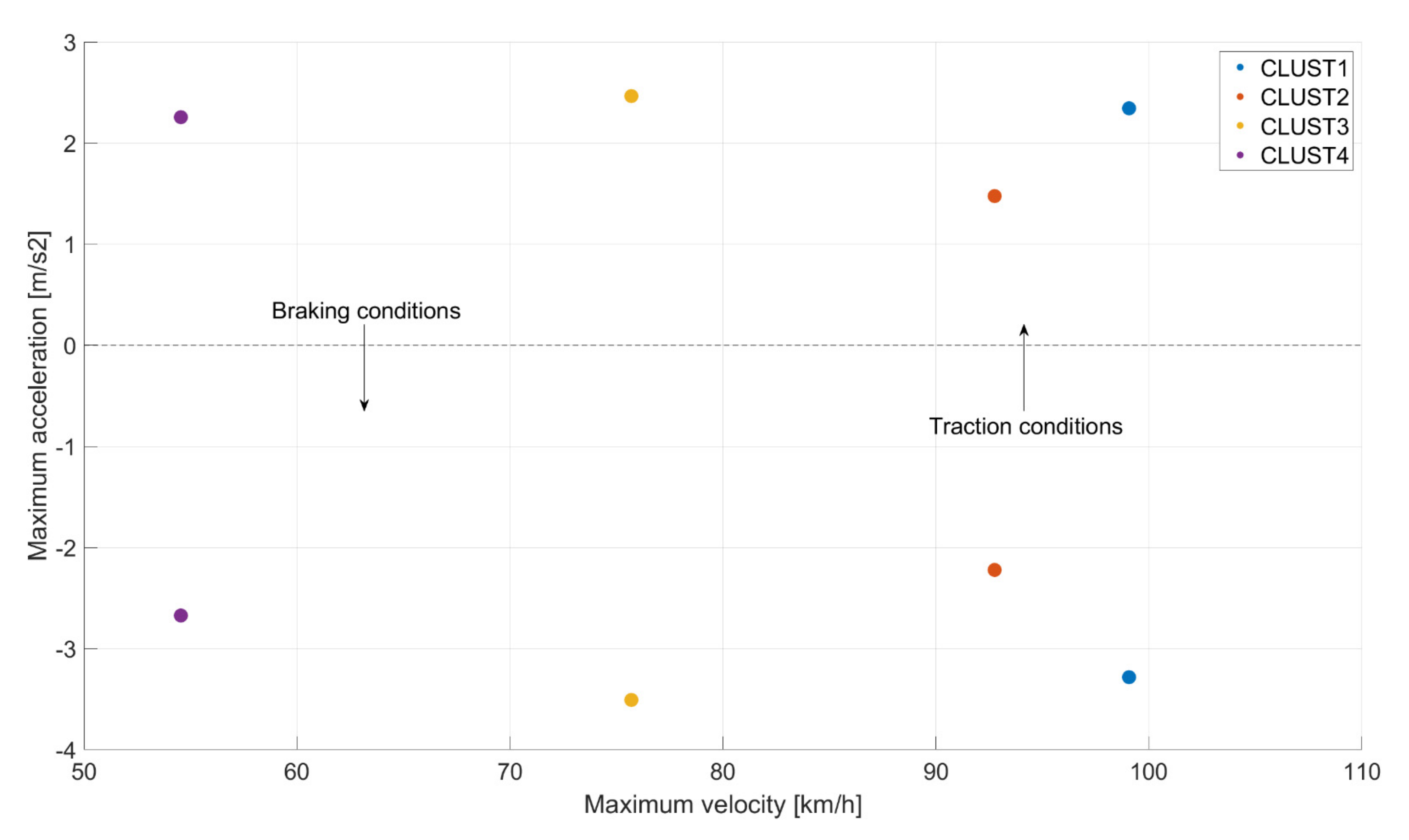
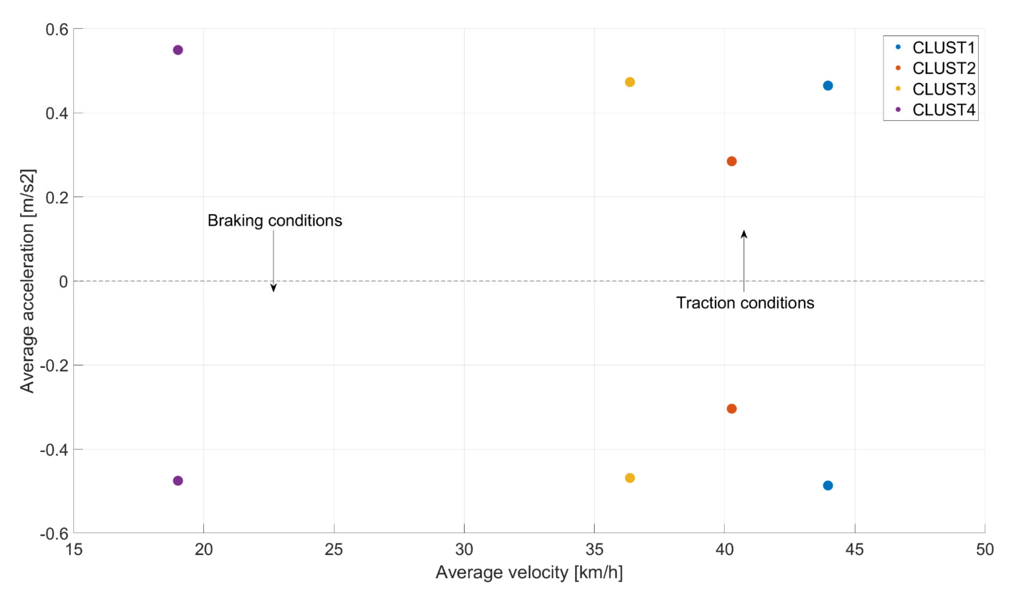
  37. Fusco, G.; Bracci, A.; Caligiuri, T.; Colombaroni, C.; Isaenko, N. Experimental analyses and clustering of travel choice behaviours by floating car big data in a large urban area. IET Intell. Transp. Syst. 2018, 12, 270–278. [Google Scholar] [CrossRef]
Figure 1. Three different exploration strategies for a Reinforcement Learning agent.
Applsci 12 00812 g001
Figure 2. Integrated modular software framework based on Reinforcement Learning for hybrid electric vehicles.
Applsci 12 00812 g002
Figure 3. Powertrain configuration of a parallel pre-transmission hybrid electric vehicle.
Applsci 12 00812 g003
Figure 4. Comparison of the vehicle velocity trajectories as a function of the mission time between CLUST1, CLUST2, CLUST3 and CLUST4.
Applsci 12 00812 g004
Figure 5. Comparison of the vehicle velocity trajectories as a function of the distance covered between CLUST1, CLUST2, CLUST3 and CLUST4.
Applsci 12 00812 g005
Figure 6. Comparison of the maximum accelerations realized in CLUST1, CLUST2, CLUST3 and CLUST4.
Applsci 12 00812 g006
Figure 7. Comparison of the average accelerations realized in CLUST1, CLUST2, CLUST3 and CLUST4.
Applsci 12 00812 g007
Figure 8. Effect of a null discount factor on the discounted return evaluated at the first time step of CLUST1.
Applsci 12 00812 g008
Figure 9. Battery SoC obtained with Q-learning in case of null discount factor during training and testing episodes.
Applsci 12 00812 g009
Figure 10. Discounted return of the training episodes calculated at the initial time step of CLUST1 for γ = 0.9.
Applsci 12 00812 g010
Figure 11. Discounted return of the training episodes calculated at 1/3 of the CLUST1 for γ = 0.9.
Applsci 12 00812 g011
Figure 12. Discounted return of the training episodes calculated at 2/3 of the CLUST1 for γ = 0.9.
Applsci 12 00812 g012
Figure 13. Battery SoC over CLUST1 evaluated throughout the first saved and last training episodes.
Applsci 12 00812 g013
Figure 14. Battery SoC over CLUST1 evaluated throughout the first saved and last testing episodes.
Applsci 12 00812 g014
Figure 15. Cumulative FC over CLUST1 evaluated throughout several training episodes.
Applsci 12 00812 g015
Figure 16. Cumulative FC over CLUST1 evaluated throughout several testing episodes.
Applsci 12 00812 g016
Figure 17. Comparison of the discounted return evaluated at the initial time step of the testing episodes for L1s and L3s.
Applsci 12 00812 g017
Figure 18. Comparison of the discounted return evaluated at 1/3 of the testing episodes for L1s and L3s.
Applsci 12 00812 g018
Figure 19. Comparison of the discounted return evaluated at 2/3 of the testing episodes for L1s and L3s.
Applsci 12 00812 g019
Table 1. Characteristics of the main vehicle and powertrain components.
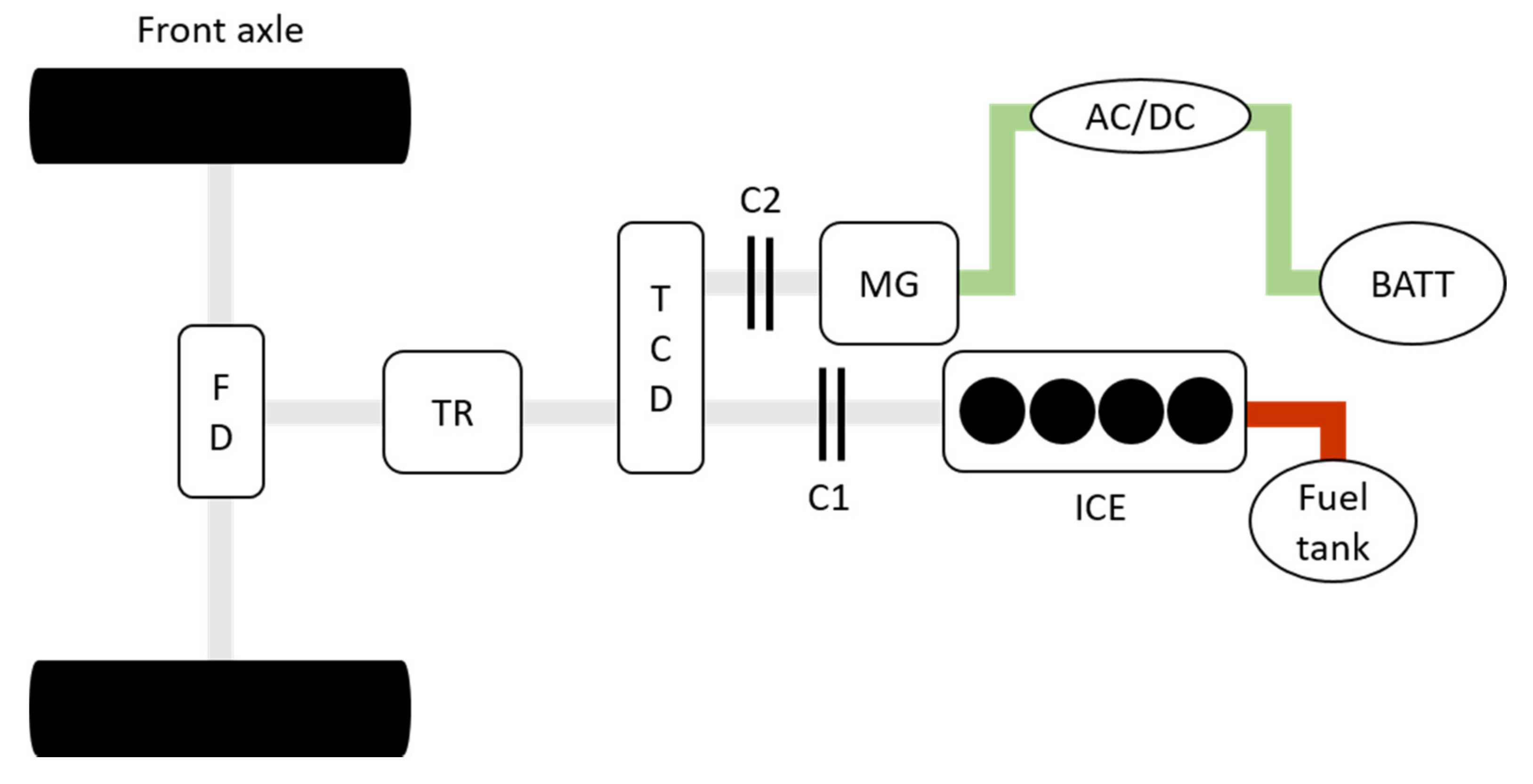
General Specifications
Vehicle classPassenger car
Kerb weight (kg)750
Vehicle mass (w/pwt components)1200
Transmission6-gears
Internal Combustion Engine
Fuel typeGasoline
Maximum power (kW (@ rpm))88 (@ 5500)
Maximum torque (Nm (@ rpm))180 (@ 1750–4000)
Rotational speed range (rpm)0–6250
Motor-generator
Maximum power (kW (@ rpm))70 (@ 6000)
Maximum torque (Nm (@ rpm))154 (@ 0–4000)
Rotational speed range (rpm)0–13500
Battery
Peak power (kW)74
Energy content (kWh)6.1
AC/DC converter efficiency (-)0.95
Table 2. Effect of the discount factor on a Q-learning based energy management system of a hybrid electric vehicle under real-world driving conditions.
DM S o C f   ( - ) FC (g)
DPQl
γ = 0.9
Ql
γ = 0.99
Ql
γ = 0.999
DPQl
γ = 0.9
Ql
γ = 0.99
Ql
γ = 0.999
CLUST10.60000.58380.59390.5904246.6229.91263.20244.47
CLUST20.60000.58260.59620.6000197.2227.19255.38263.46
CLUST30.60000.58170.5754-152.6173.02169.26-
CLUST40.60000.58190.60190.597453.952.07106.5693.81
rFC (g) Δ F C (%)
CLUST1246.6253.21272.02258.27-2.6810.314.73
CLUST2197.2252.28260.9263.46-27.9332.3033.60
CLUST3152.6199.33204.7--30.6234.14-
CLUST453.978.21106.5697.59-45.1097.7081.06
Table 3. Reward shaping analysis considering γ = 0.9.
γDM S o C f   ( - ) FC (g)
DPR1R2aR2bR2cR3DPR1R2aR2bR2cR3
0.9CLUST10.60000.5838---0.5977246.6229.91---259.89
CLUST20.60000.5826---0.6000197.2227.19---282.63
CLUST30.60000.5817----152.6173.02----
CLUST40.60000.5819---0.588453.952.07---66.52
rFC (g) Δ F C (%)
CLUST1246.6253.21---263.13-2.68---6.70
CLUST2197.2252.28---282.63-27.93---43.32
CLUST3152.6199.33-----30.62----
CLUST453.978.21---83.29-45.10---54.53
Table 4. Reward shaping analysis considering γ = 0.99.
γDM S o C f   ( - ) FC (g)
DPR1R2aR2bR2cR3DPR1R2aR2bR2cR3
0.99CLUST10.60000.5939---0.6018246.6263.20---280.80
CLUST20.60000.5962---0.6031197.2255.38---254.28
CLUST30.60000.5754----152.6169.26----
CLUST40.60000.6019---0.598453.9106.56---88.48
rFC (g) Δ F C (%)
CLUST1246.6272.02---280.83-10.31---13.88
CLUST2197.2260.9---254.28-32.30---28.95
CLUST3152.6204.7-----34.14----
CLUST453.9106.56---90.86-97.70---68.57
Table 5. Reward shaping analysis considering γ = 0.999.
γDM S o C f   ( - ) FC (g)
DPR1R2aR2bR2cR3DPR1R2aR2bR2cR3
0.999CLUST10.60000.5904---0.6011246.6244.47---293.15
CLUST20.60000.6000---0.6049197.2263.46---266.82
CLUST30.6000----0.5795152.6----185.51
CLUST40.60000.5974---0.598253.993.81---95.23
rFC (g) Δ F C (%)
CLUST1246.6258.27---293.15-4.73---18.88
CLUST2197.2263.46---266.82-33.60---35.30
CLUST3152.6----214.99-----40.88
CLUST453.997.59---97.86-81.06---81.56
Table 6. Results produced by a sensitivity to α considering α = 0.1, α = 0.5 and α = 0.9.
DM S o C f   ( - ) FC (g)
DPQl
α = 0.1
Ql
α = 0.5
Ql
α = 0.9
DPQl
α = 0.1
Ql
α = 0.5
Ql
α = 0.9
CLUST10.60000.57780.60140.5838246.6226.51298.62229.91
CLUST20.60000.58320.60210.5826197.2207.42280.22227.19
CLUST30.6000--0.5817152.6--173.02
CLUST40.6000-0.60030.581953.9-101.8952.07
rFC (g) Δ F C (%)
CLUST1246.6258.65298.62253.21-4.8921.092.68
CLUST2197.2231.65280.22252.28-17.4742.1027.93
CLUST3152.6--199.33---30.62
CLUST453.9-101.8978.21--89.0445.10
Table 7. Effects of a variation of the exploration strategy considering L1, L2 and L3.
DM S o C f   ( - ) FC (g)
DPL1L2L3DPL1L2L3
CLUST10.60000.58380.60200.6017246.6229.91309.01269.35
CLUST20.60000.58260.60200.6022197.2227.19299.63255.55
CLUST30.60000.5817--152.6173.02--
CLUST40.60000.58190.60100.601053.952.0788.0990.33
rFC (g) Δ F C (%)
CLUST1246.6253.21309.01269.35-2.6825.319.23
CLUST2197.2252.28299.63255.55-27.9351.9429.59
CLUST3152.6199.33---30.62--
CLUST453.978.2188.0990.33-45.1063.4367.59
Table 8. Results by L1s and L3s exploration strategies on CLUST1.
DM S o C f   ( - ) FC (g)rFC (g)
L1sL3sL1sL3sL1sL3s
CLUST10.60140.6010267.74286.08267.74286.08
Publisher’s Note: MDPI stays neutral with regard to jurisdictional claims in published maps and institutional affiliations.

