Article

Outpatient Appointment Optimization: A Case Study of a Chemotherapy Service

1
Opta LP S.A.S., 2 Rue Gustave Eiffel, 10430 Rosieres-pres-Troyes, France
2
Computer Sciences and Digital Society Laboratory (LIST3N), Université de Technologie de Troyes, 12 Rue Marie Curie, CS 42060, 10004 Troyes, France
3
Chaire Connected Innovation, Université de Technologie de Troyes, 12 Rue Marie Curie, 10004 Troyes, France
*
Author to whom correspondence should be addressed.
Appl. Sci. 2022, 12(2), 659; https://doi.org/10.3390/app12020659
Submission received: 17 November 2021 / Revised: 3 January 2022 / Accepted: 4 January 2022 / Published: 10 January 2022
(This article belongs to the Section Computing and Artificial Intelligence)

Abstract

:

Featured Application

This study provides a procedure-detailed scientific approach for the outpatient planning problem at the chemotherapy department.

Abstract

In this paper, we study a complex outpatient planning problem in the chemotherapy department. The planning concerns sequences of patients’ treatment sessions subject to exact in-between resting periods (i.e., exact time-lags). The planning is constrained by the hospital infrastructure and the availability of medical staff (i.e., multiple time-varying resources’ availability). In order to maximize the patients’ service quality, the objective of the function considered is to minimize the total wait times, which is equivalent to the criteria for minimizing the total completion time. Our main contribution is a thorough analysis of this problem, using the Hybrid Flow Shop problem as a theoretical framework to study the problem. A novel Mixed Integer Linear Programming (MILP) is introduced. Concerning the resolution methods, priority-based heuristics and an adapted genetic algorithm (GA) are presented. Numerical experiments are conducted on historical data to compare the performances of the approximate resolution methods against the MILP solved by CPLEX. Numerical results confirm the performances of the proposed methods.

1. Introduction

According to Hesaraki [1], there are two treatment settings in hospitals: inpatient care and outpatient care. Inpatient care requires more than one day of hospitalization. Outpatient care concerns patients who are admitted to and leave hospitals on the same day. While inpatient care demands dedicated resources such as a bed or a room with equipment for a single patient, outpatient care allows for reusing the same resources for several patients a day, thus increasing the utility and the flexibility of the hospital infrastructure. A challenge arises with the growing number of patients’ demands: ensuring the service capability of human and infrastructural resources while maintaining the quality of services.
In this work, we study the outpatient planning problem under medical resources. The hybrid flow shop problem is applied as our theoretical framework for the problem studied. The case-study context and data are provided by the service of Outpatient Care of Pneumonology–Hematology–Oncology (Troyes Hospital Center, France).
The main contributions of this work are as follows: (1) a most detailed procedural analysis, to the best of our knowledge, of a chemotherapy planning problem; (2) a novel mixed-integer linear programming model that takes into account the exact time-lag and time-varying resource constraints; (3) adapted heuristics and a genetic algorithm allowing for parallel computation to reduce time computation proposed to efficiently solve the problem studied.
This paper is organized as follows: Section 2 provides a detailed description of the problem following by a complexity analysis. Next, Section 3 gives the overview of the outpatient scheduling/planning, especially the chemotherapy. The Mixed Integer Linear Programming (MILP) model from our previous work [2] is detailed in Section 4. Section 5 is dedicated to resolution methods: eight priority-based heuristics and a genetic algorithm. Section 6 specifies the test protocol and the numerical results to gauge the performances of different approaches. Finally, Section 7 concludes this paper with our remarks and states our future works.

2. Problem Description

This section provides a detailed description of the problem followed by a classification of the problem and a complexity analysis.

2.1. Outpatient Scheduling Problem

The outpatient scheduling at the chemotherapy service includes two subproblems, according to Condotta and Shakhlevich [3]. In the first problem, in which the time horizon is considered by the number of days, the scheduler must decide the starting time of a sequence of treatment sessions (as known as appointments) and rest days in-between (Figure 1). The second planning problem has the time horizon limited by a day and consists of a four-stage process requiring multiple resources at each stage (Figure 2).
The first subproblem considers, for each patient, a complete chemotherapy outpatient therapy, which is called the multi-day pattern. The therapy comprises several treatment sessions (i.e., appointments) distanced by predefined resting time windows for healing, as illustrated in Figure 1. These inter-appointment periods are fixed so that the patient’s health recovers for the next session. For the sake of brevity, this sequence is denoted as a cycle of a patient.
The second subproblem handles the scheduling on the day of the appointment, decided by the first subproblem. After being admitted, the patient consults a doctor to check up on her/his current health condition. If the patient is judged to be not healthy enough to receive the treatment, the current session is rescheduled to another day. Otherwise, the patient follows a nurse to an available seat (a bed or an armchair). In parallel, the required chemotherapy drug is prepared at the pharmacy unit. Once the drug is ready, the patient proceeds to receive the treatment under the monitoring of a nurse.
However, in some exceptional cases, the treatment session does not require a consultation in the same day because this consultation can be made in advance. In this case, the consulting time of the patient is considered zero. Furthermore, occasionally, the mixing drug step is permitted to proceed one day in advance so that the waiting time can be reduced. The Gantt diagram in Figure 3 illustrates those operations.
Both subproblems have time-varying resource availability, illustrated as in Figure 4. Since the processing of each stage requires one or multiple resources, the variation in resources implies the maximal number of patients that the service can handle simultaneously. In this problem, four types of resources are considered:
  • Pharmacy: a resource only available during the predefined opening hours. The capacity of the pharmacy is considered unlimited.
  • Doctor: a discrete time-varying resource. A doctor can receive a maximum of one patient at a time.
  • Nurse: a discrete time-varying shared resource. Each nurse can install a patient to a seat or simultaneously monitor at most Ψ patients.
  • Seat: a constant renewable resource. Each patient occupies a seat from the beginning of installation until the end of the session of care.

2.2. Problem Categorization

We denote the problem using the Graham notation α | β | γ [4].
For each session, the patient should go through four stages, as mentioned earlier (Figure 2 and Figure 3), and then, the problem belongs to the family of Flow Shop problems. In addition, according to the capacity of different types of resources, the last stage (monitoring) can be executed for multiple patients in parallel. The problem is classified to be a Hybrid Flow Shop scheduling problem. Since each care session has four operations, we denote α = F H 4 .
The resource constraints are denoted as r e s λ σ ρ according to Blazewicz et al. [5], with new modifications introduced by Weglarz [6]. There are four types of resources required for the execution of jobs ( λ = 4 ). No bound on the resource capacities is known a priori ( σ = · ). The requirement of resources is bounded correspondingly to the stage ( ρ = 1 ): one doctor for consultation, one pharmacy unit for drug mixing, one nurse and one chair for installation, and  1 / Ψ nurse (in terms of capacity Ψ ) and one chair for monitoring. The resource constraints notation is then r e s 4 · 1 .
The final job constraint is the waiting time between two treatment sessions of a patient (Figure 1). An outpatient chemotherapy cycle requires the patient in question to rest a certain number of days before entering the next session. In the literature, this constraint is described as the time-lag constraints, which are denoted as l j j [7,8]. The time-lag is a generalization of the precedence constraint where one job has to wait an amount of time before processing, depending on another job. Due to the technical aspects of the chemotherapy care, we are only interested in the number of days between two consecutive jobs.
The objective of our studied problem is to maximize the quality of service. In this case, we tend to reduce the mean waiting time of the patients, which is equivalent to minimizing the total completion time [9].
In summary, the problem is noted as:
F H 4 | l j j , r e s 4 · 1 | C j

2.3. Problem Complexity

By assuming that the input is only patients with a single session and that consultation and installation time are zero, the considered problem without resources constraints is reduced to the two stages Flow Shop problem, which is NP-hard [10]. Furthermore, the resource variation is usually seen as an element that makes the planning/scheduling problem harder to solve [11]. Our problem thus should be at least NP-hard.

3. Literature Review

Healthcare services have been receiving a growing number of papers covering several major domains in response to many complex problems from the increasing patients’ demands under limited and scarce resources. Multiple reviews [12,13,14,15,16,17,18,19] have shown an extensive view about typical challenges regarding multiple aspects, levels, and criteria.
The hybrid approach of the branch-and-bound algorithm and the constraint programming technique in [20] proposes exact solutions for the generic integrated problem of employee timetabling and job-shop scheduling. The work is then applied to the outpatient chemotherapy scheduling problem, yielding significant results. The work of Condotta and Shakhlevich [3] considers the recovery duration after each session (multi-day time-lag) and the intervention during the monitoring step (intraday time-lag) by resolving two ILP models corresponding to multi-day and intraday subproblems over the rolling horizon. Hahn-Goldberg et al. [21], on the other hand, proposed resolution methods based on Constraint Programming and MIP that yield applicable performance. Liang and Turkcan [22] tackled it using a multi-objective optimization, providing a helpful spreadsheet decision-making solution for strategical clinic management. The branch-and-price algorithm of Legrain et al. [23] founds an application in the nurse rostering problem. Under the assumptions that the pharmacy unit and oncologists are abundant, the MILP model by Hesaraki [1] focuses primarily on the last two stages because efficiently allocating nurses in a day is more critical and complex. Then, the method aggregates the time-lag progressively by applying a rolling horizon and schedule template to construct the long-term planning. Overall, few papers consider the problem with multiple types of resources and time-varying resource availability.
On the other hand, a quick and approximate solution’s applicability in practical cases has attracted the development of heuristic and meta-heuristic. Menting and Menting [24] built several heuristic algorithms to enhance the schedule of affecting resources (nurses and seats) to patients after applying LPT rule combined with First Fit Strategy. The resolution time is less than several seconds, resulting in a good planning tool for the local hospital in daily usage. The review of Marynissen and Demeulemeester [19] lists multiple meta-heuristic approaches for multi-appointment planning and, in particular, chemotherapy scheduling. The latter invokes multiple resources and requires repeating treatment sessions over a long horizon.
As far as we know, there is a lack of work in the literature that studies all four mentioned stages. As indicated in Table 1, while some work considers the multi-day subproblem (time-lag), few include all stages (intra-day subproblem) and required resources. That is the reason why our previous work’s model [2] is the most detailed in terms of care operations so far, according to our knowledge.

4. Mathematical Model

The mathematical models of Hesaraki [1] and Condotta and Shakhlevich [3] deal principally with constant resources, which cannot be adapted to our problem where the resources vary over time. For this reason, we develop another formulation using disjunctive binary variable technique. This modeling approach brings us some benefits. The variation of resources can be wholly taken into account and can be extensible to any number of discrete resources types. Reordering operations can be made without complete modification of resources constraints. Readers are referred to the work of Nguyen et al. [26] for more details.
Let us denote the disjunctive binary variable as follows:
σ i , k , j , h o = 1 if operation o of appointment k of patient i starts at time h on day j 0 otherwise
χ i , k , j , h o = 1 if operation o of appointment k of patient i ends at time h on day j 0 otherwise
The detailed notations to the problem are stated in Table 2. With such a notation, we can describe the fundamental measures of a given treatment session k of patient i mathematically:
  • Each operation o can be started and ended only once:
    j J h H σ i , k , j , h o = 1
    j J h H χ i , k , j , h o = 1
  • The processing time p i , k , j , h o of an operation o must be equal to the difference between the starting time σ i , k , j , h o and the completion time χ i , k , j , h o :
    σ i , k , j , h o = χ i , k , j , h + p i , k o o
  • Given a date j, the completion indicator variable h h χ i , k , j , h o checks whether the operation o is completed by the moment h. Therefore, if an operation o ^ succeeds o, the starting time of o ^ must not exceed o’s completion indicator:
    σ i , k , j , h o ^ h h χ i , k , j , h o
  • Since h H χ i , k , j , h D indicates if the session k happens on day j, one can use the following formula to extract the index of the day when the treatment session happened:
    j i , k = j J \ 0 j × h H χ i , k , j , h D
    One can find the completion time of a process by a similar manner:
    h i , k = j J \ 0 h H h × χ i , k , j , h D
    From (4), (7) and (8), we can rewrite the completion time of a session k by multiplying j i , k the number of passing days by H the number of timeslots per day then adding up with h i , k the elapsed time of the treatment:
    C i , k = H × j i , k 1 + h i , k 1 = H × j J \ 0 j × h H χ i , k , j , h D j J \ 0 h H χ i , k , j , h D + + j J \ 0 h H h × χ i , k , j , h D j J \ 0 h H χ i , k , j , h D = H × j J \ 0 h H j 1 × χ i , k , j , h D + j J \ 0 h H h 1 × χ i , k , j , h D = j J \ 0 h H H × j 1 + h 1 χ i , k , j , h D
  • Given a date j, the resource usage at the time h is determined by the execution of operation o, which is calculated by the sum of the difference of the starting time indicator variable σ i , k , j , h o and the completion time indicator variable σ i , k , j , h o from time 0 to h: h h σ i , k , j , h o χ i , k , j , h o .
From these formulas, we obtain the MILP model as follows:
Minimize i P k Θ i j J \ { 0 } h H H × j 1 + h 1 × χ i , k , j , h D Subject to :
j J h H σ i , k , j , h o = j J h H χ i , k , j , h o = 1 i P , k Θ i , o O
χ i , k , j , h + p i , k o o = σ i , k , j , h o i P , k Θ i , o O , j J , h H
h H σ i , k , j , h o = h H χ i , k , j , h o i P , k Θ i , o O , j J
h H σ i , k , j , h A = h H σ i , k , j , h B = h H σ i , k , j , h D i P , k Θ i , j J
σ i , k , 0 , h o = χ i , k , 0 , h o = 0 i P , k Θ i , o { A , B , D } , h H
σ i , k , j , h B h h χ i , k , j , h A i P , k Θ i , j J , h H
j J : j e i , k C j j h H σ i , k , j , h C h H σ i , k , j , h A i P , k Θ i , j J , h H
1 e i , k C σ i , k , j , h C h h χ i , k , j , h A i P , k Θ i , j J , h H
σ i , k , j , h D h h χ i , k , j , h B i P , k Θ i , j J , h H
σ i , k , j , h D j J : j e i , k C j < j h H χ i , k , j , h C + h h χ i , k , j , h C i P , k Θ i , j J , h H
h H σ i , k + 1 , j + Δ k + 1 i , h A = h H σ i , k , j , h A i P , k 1 , , n i 1 , j J : j + Δ k + 1 i J
M i P k Θ i h h σ i , k , j , h B χ i , k , j , h D j J , h H
D j , h i P k Θ i h h σ i , k , j , h A χ i , k , j , h A j J , h H
I j , h i P k Θ i h h σ i , k , j , h B χ i , k , j , h B + σ i , k , j , h D χ i , k , j , h D / Ψ j J , h H
F j , h h h σ i , k , j , h C χ i , k , j , h C i P , k Θ i , j J , h H
Since we aim to reduce the total waiting time of the patient in the hospital, the objective function is the total completion time minimization (10), expressed by Equation (9). We summarize here the explication of each group of constraints:
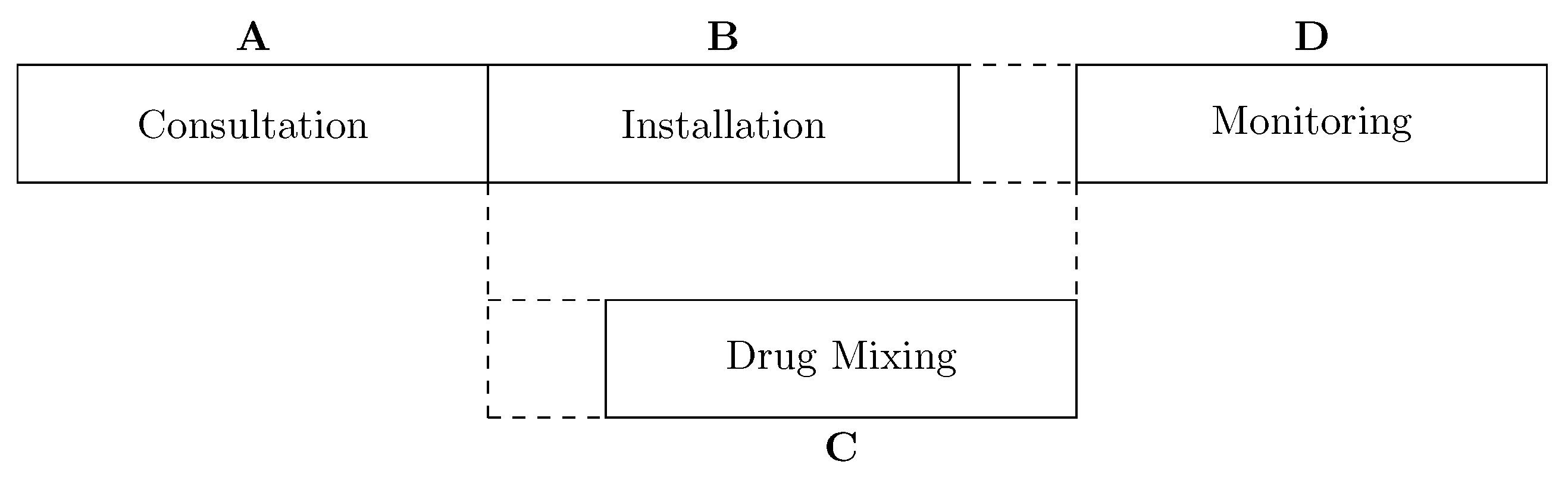
  • Operations: (11) obligates any operation to start and end exactly once on the horizon, according to (3). (12) makes each operation non-preemptive, which means that, once an operation starts, it must be processed without interruption. Equation (13) makes their start and end dates the same (outpatient regime). For each session, three stages (consultation, installation, and administration) are on a same day (14). However, since day 0 is a dummy day to allow for mixing the drug in advance, if possible, for day 1, these three steps are prohibited on day 0 (15).
    According to the order of operations, the installation never precedes consultation (16). The mixing, if a priori preparation is authorized ( e i , k C = 1 ), can proceed at most one day before the day of treatment session (17); otherwise, it follows the end of consultation (18). Finally, monitoring starts when the patient has been fully installed (19) and the drug is available (20).
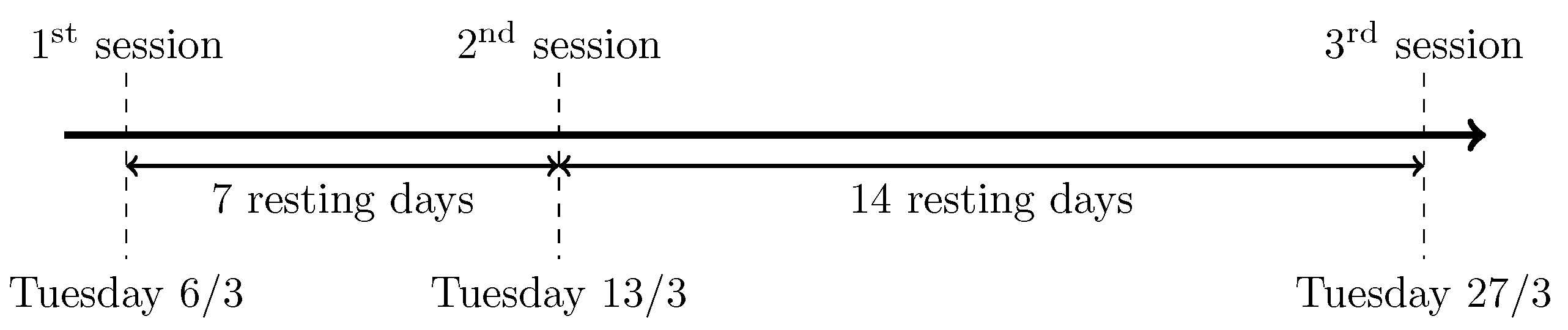
  • Appointments: Each patient has a set of appointments in which the time-lags have been decided beforehand in terms of days (21).
  • Seats: A patient occupies one seat from the beginning of installation until finishing the monitoring (22).
  • Doctors: One doctor takes in one patient at a time (23).
  • Nurses: A nurse can either install a patient into a seat or monitor a group of Ψ patients (24).
  • Pharmacy: Unlimited orders are allowed to process in parallel as long as the mixing procedures are in the pharmacy’s opening time (25).

5. Resolution Methods

Although the MILP model for our problem defined at Section 4 gives exact solutions with the solver CPLEX, the resolution time increases exponentially as the instance size grows. Thus, we seek other approaches with a more reasonable resolution time. We present in this section eight priority rules and a genetic algorithm adapted to the problem.

5.1. Dispatching Rule Heuristics

Due to the time-lag constraint, one must always ensure the exact waiting time between two patient sessions. With First Fit Strategy (FFS) [27], we can find a resource, precedence, and feasible planning for a sequence of appointments of a patient by scheduling as soon as possible while ensuring the time-lag and resources’ availability for the patient. In addition, the time-lag is only applied to the appointments of each patient. Hence, it is sufficient to represent the problem’s instance as an orderly list of patients.
Since the SPT rule is a well-known rule for 1 | | C j [28] by prioritizing the job with lower processing time, we first define the priority value total processing time as the sum of the entire elapsed time for all steps at all appointments.
We also define the ideal total processing time, a variation that takes into account the flexibility of jobs in the ideal case where we process without resource constraints:
I P T i , k : i d e a l t o t a l p r o c e s s i n g t i m e of appointment k of patient i = p i , k A + max p i , k B ; 1 e i , k C p i , k C + p i , k D = p i , k A + max p i , k B ; p i , k C + p i , k D if C is not allowed to preproceed p i , k A + p i , k B + p i , k D otherwise I P T i = k Θ i I P T i , k : i d e a l t o t a l p r o c e s s i n g t i m e of patient i
Finally, note that, if we delay the first session by one day, the time-lag pushes the second session an equal amount, resulting in an increase of two days ( 2 × H time slots) in total on the objective (10). In other words, delaying the first session of patient i by one day increases the objective (10) by at least n i × H . For that reason, we see by intuition that prioritizing long requests reduces the objective substantially. Combining with the idea of MTS (Most Total Successor) [29], we construct hence the RLIPT priority value, as a lexicographical order n i ; I P T i so that the lengthier cycle (greater n i ) is prioritized, tie-broken by the ideal total processing time ( I P T i ) as processing the shorter jobs first might be beneficial. There are thus four possible variations of ordering (all listed for the sake of completeness) RLIPT-DD (both n i ; I P T i in decreasing order), RLIPT-II (both n i ; I P T i in increasing order), RLIPT-DI (decreasing order of n i then increasing order of I P T i ), and RLIPT-ID (increasing order of n i then decreasing order of I P T i ).
In summary, we sort patients’ planning requests in increasing (or decreasing) order of priority values defined formally in Table 3. The heuristics to examine are SPT, LPT, SIPT, LIPT, RLIPT-DD, RLIPT-II, RLIPT-DI, and RLIPT-ID.

5.2. Genetic Algorithm

Meta-heuristics methods received more attention as its performance increased significantly to solve resource-constrained project scheduling for healthcare services [12,18,19,30]. In this problem, since it is straightforward to calculate the planning given a list of patients’ entrance using FFS, we decided to use genetic algorithm to generate numerous lists and to converge toward the best.
The main elements of our GA are as follows:
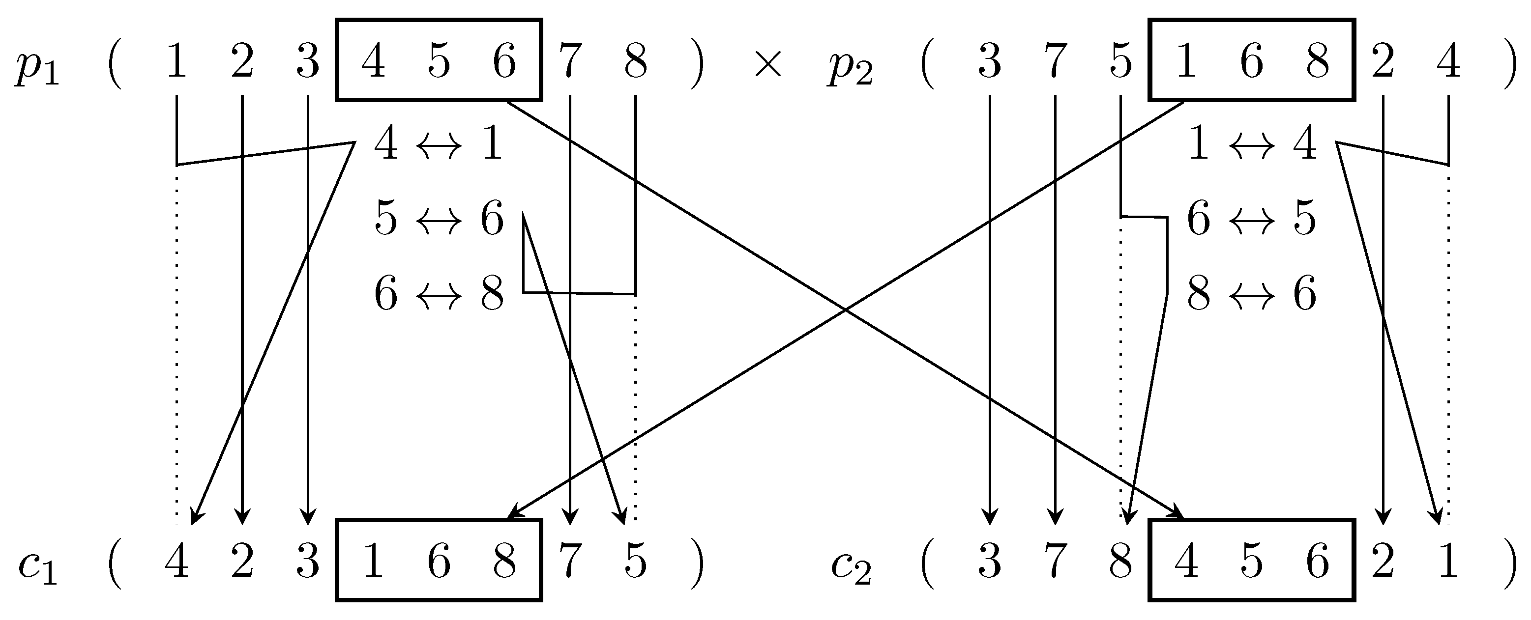
  • Encoding: We encode a chromosome as an ordinal sequence of patients, i.e., a chromosome is a permutation of the list of patients because we try to determine a priority list to schedule with FFS, similar to the priority-based heuristics earlier.
  • Initial population: Given the permutation encoding scheme above, the initial population is created by randomly shuffling N P times the set of patients 1 , 2 , , n .
  • Selection: Tournament Selector (TS) is chosen because of its O ( n ) time complexity and easy parallelization for speeding up calculation in practical use. Furthermore, while a large tournament results in loss of diversity, a binary tournament performance is generally inferior to a three-tournament. Hence, the tournament size is fixed by 3.
    Let us denote F O 0 F O 1 as the fraction of population selected to give offspring.
  • Crossover: Due to the permutation encoding, the order of requests is critical to deduce the planning. Hence, we adopt Partially Mapped Crossover (PMX, Figure 5), first introduced by Grefenstette [31], so that a potentially good local order is transferred from parent to child.
  • Mutation: The offspring are then applied Partial Mutator Shuffle (PSM, known as Swap Mutator, Figure 6) with probability P M [32], so that a new order not in the current research neighborhood may appear.
  • Population management: Denote F S = 1 F O as the fraction of current population that we want to keep for the next generation in order to preserve diversity. The population is kept constant by combining the children ( F O × N P ) and parents ( F S × N P ).
  • Stop condition: The process is terminated after N G successive generations that the objective value of the incumbent has not been changed.
We chose F O , F S = 0.5 , 0.5 for a balance of the intensity and the diversity of the search. The process stops after continuously staying at an objective value for long enough. The preliminary numerical experiments show that the incumbent rarely descends after 100 generations. Therefore, we can make the GA finish earlier by terminating it after a certain number of times, obtaining the same objective value instead of a fixed number of generations in total.

6. Computational Results

This section presents the benchmark based on historical data and then calibrates the proposed genetic algorithm. Finally, the results are shown and discussed.

6.1. Instance Generation

We use the test protocol and instances introduced in our previous work [2]. The dataset is published at [34]. Each instance has two sets of data: resources availability (seats M, doctors D ( j , h ) , nurses I ( j , h ) , pharmacy unit F ( j , h ) ), and planning requests ( Θ 1 , Θ 2 , , Θ n with n number of patients).
The generator’s data is based on the data of Hospital Center of Troyes (CHT) in France (2020). The instances are generated as follows:
  • The number of seats M is 30.
  • Horizon is 4 weeks ( J = 28 ), and each day consists of 22 time slots ( H = 22 ).
  • The maximal number of patients a nurse can monitor simultaneously: Ψ = 6 .
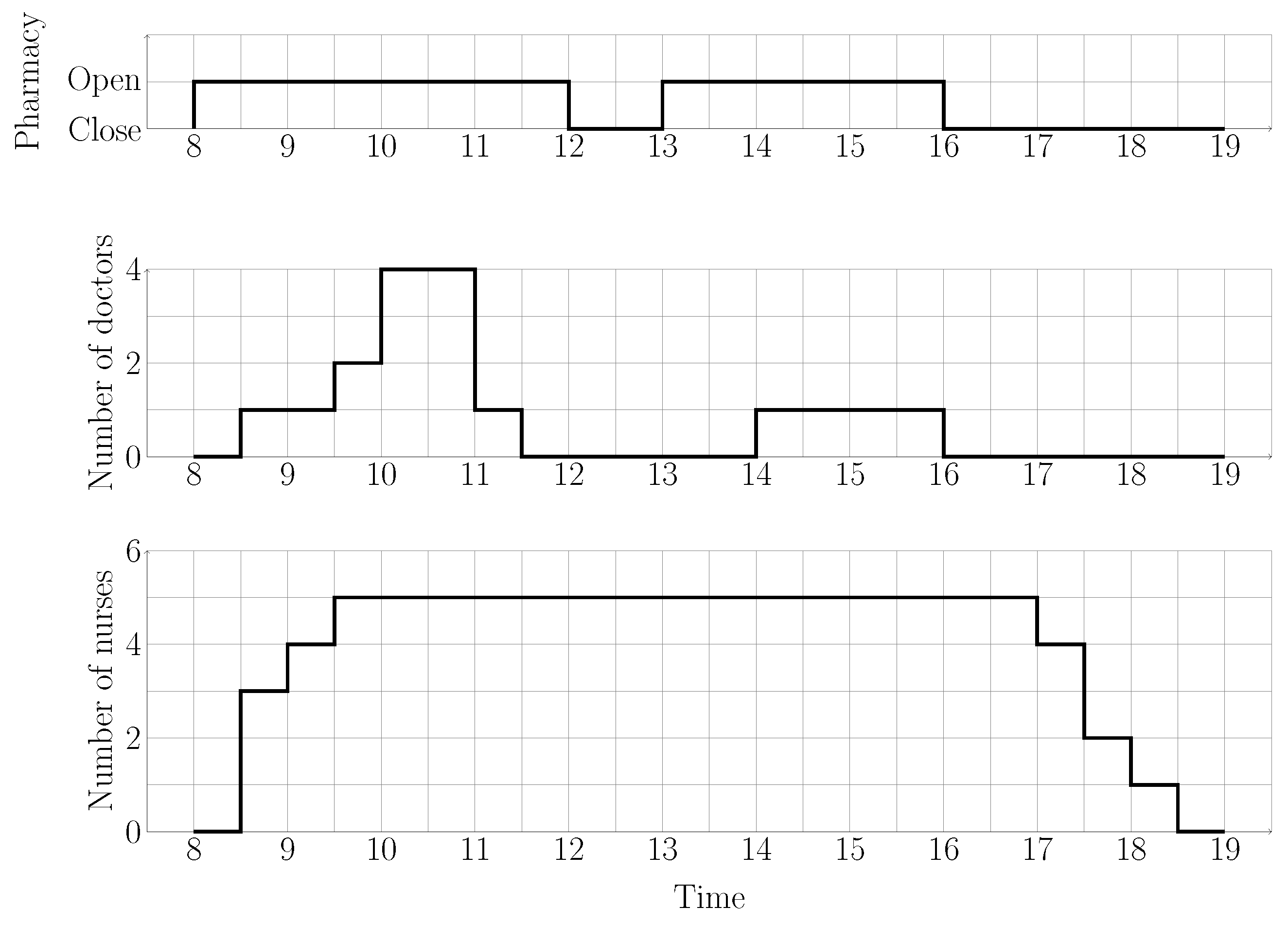
  • Human resources’ presence are generated using a discrete uniform distribution ( unif ), of which the amount is an integer number varying between 0 (unavailable) and the maximum (fully available), noted as unif 0 ; M with M the major bound the resource capacity. Historical data gives us N D = 5 , N I = 6 maximal number of doctors and nurses, respectively. Unlimited resource such as pharmacy could use 1 to represent to up state (open) and 0 for down state (close).
    We divide further the resources’ availability into four different scenarios to represent the reality:
    -
    Uniform: D j , h unif 0 ; N D ; I j , h unif 0 ; N I ; F j , h unif 0 ; 1 .
    -
    Daily: Similar to Uniform, but the distribution is repeated daily.
    -
    Weekly: Similar to Uniform, but the distribution is repeated weekly.
    -
    Weekend: Similar to Uniform but no resource available on weekends, simulating the current working schedule at the service.
  • For each request of indexed i patient, we define the following:
    -
    Number of required sessions Θ i unif 1 ; 3 .
    -
    Time-lag Δ i , k unif 1 ; 3 , except  Δ i , 1 = 0 .
    -
    Consultation time p i , k A unif 0 ; 1 (yes or no).
    -
    Installation time p i , k B = 1 .
    -
    Drug mixing time p i , k C unif 0 ; 3 .
    -
    Authorization of a priori drug mixing e i , k C unif 0 ; 1 (yes or no).
    -
    Treatment time p i , k D unif 0 ; 3 .
  • N a , which is the total number of treatment sessions, takes a value from {15; 30; 60; 90; 120; 150; 180; 210}. In order to avoid service congestion, given the limited resources, we have fixed the maximum number of treatment sessions to 210.
Using the generator implemented by Java 8 with its native random engine, we created ten instances for each scenario each N a , resulting in 320 test instances in total.
All of the numerical tests were executed on the same machine with CPU Intel Core i7–9750H (2.6 GHz∼4.5 GHz), and the time limit and the specific implementation of each method are defined as follows:
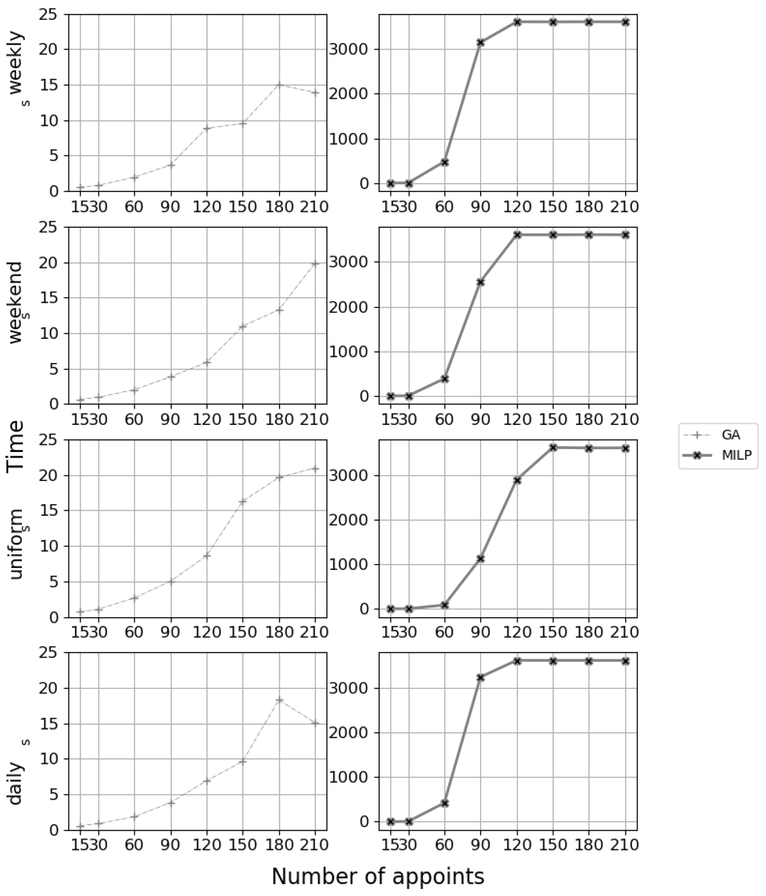
  • Solver CPLEX 12.10 solves the MILP within a time limit of 1 hour by using one CPU thread.
  • Heuristic approaches are implemented purely on Java 8.
  • Genetic algorithm’s implementation based on Jenetic library 5.0 [35].

6.2. Calibration on the Genetic Algorithm
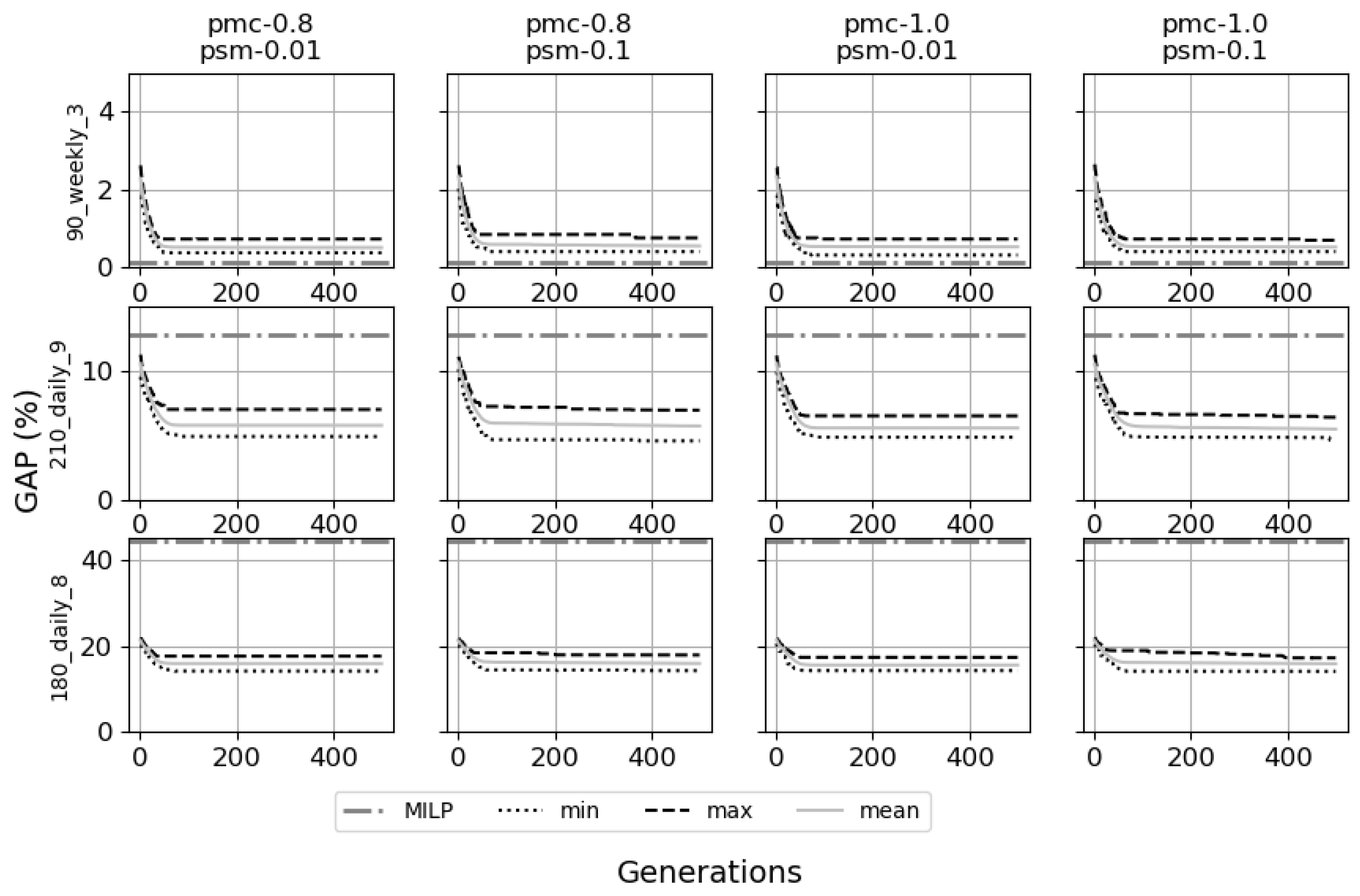
For each generated instance, we assign it to a difficulty level. The estimation of the difficulty level was based on the GAP found by MIP resolution with CPLEX after one hour of resolution. Three test instances were selected to represent the different levels of difficulty:
  • Easy (low GAP): 90 weekly 3 ( G A P = 0.10 % ).
  • Normal (medium GAP): 180 daily 8 ( G A P = 12.74 % ).
  • Hard (high GAP): 210 daily 9 ( G A P = 44.40 % ).
First, N P = 1000 was chosen for a large enough population. We observed the incumbent after 500 generations before picking a suitable number of steady generation N G .
Furthermore, because  P M is usually small and P C is frequently high, we tried the test with P M { 0.01 , 0.1 } and P C { 0.8 , 1.0 } . For each instance and tuple P C ; P M , we ran Algorithm 1 30 times and recorded the best objective value in order to trace the convergence.
In general, as we can see in Figure 7, the genetic algorithm generally converges after 100 generations. Therefore, we chose N G = 100 .
Algorithm 1: Pseudo-code for the genetic algorithm
Applsci 12 00659 i001
Furthermore, the GAP values of multiple runs on the same parameters stay close together, as we can see in Figure 7, and the difference between the best (min GAP) and the worst (max GAP) found objective values is always under 5% after 100 generations. Thus, the GA is converged (i.e., stable) with the corresponding parameters.
We observe a general decrease of final GAP when the mutator probability P M going from 0.01 to 0.1 and the cross-over probability P C increasing from 0.8 to 1.0 (Table 4 and Figure 7). Hence, the choice P C ; P M = 1.0 ; 0.1 is reasonable.

6.3. Numerical Test Results

The relative gap for method m on an instance is calculated using the following formula:
GAP m = objective value found by m Optimal objective value or best LB found by MILP 1 × 100 %
Figure 8 and Table 5 show similar behaviors for the different heuristic methods with small instances ( N a < 90 ). However, when the total number of treatment sessions grows ( N a 90 ), CPLEX cannot find an optimal solution within the limit of 1 hour due to exponentially increased combinations (Figure 9). Additionally, from this point, the performance of solving methods can be grouped into three distinct tiers:
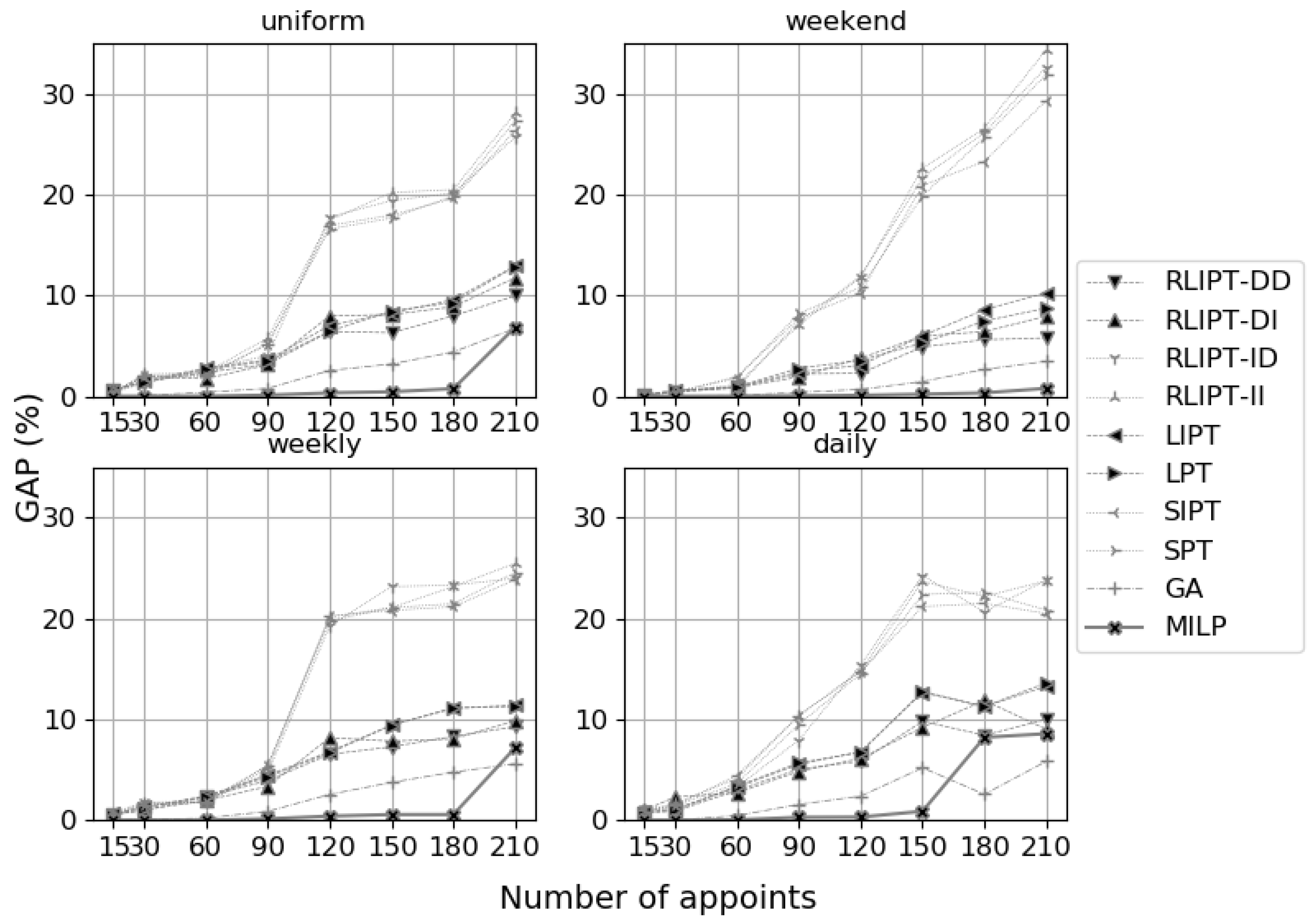
  • Low performance: including RLIPT-ID, RLIPT-II, SIPT, SPT in which the GAP vastly climbed from under 10 % to over 20 % , even 35 % in weekend’s scenario.
  • Medium performance: including RLIPT-DD, RLIPT-DI, LIPT, LPT, in which the GAP increased arguably slower than low group and stayed overall below 15 % .
  • Good performance: including MILP and GA, which in most cases give lower GAPs than the medium group, generally under 10 % .
In general, CPLEX is effective for solving the proposed MILP. Nevertheless, when the problem grows in size and resource availability congestion appears, the GA method yields better performance. Furthermore, GA is better in terms of execution time (Figure 9 and Table 6).
Finally, regarding the heuristics, we can see their GAP is decided by how they prioritized the complicated jobs regarding the heuristics. The low group puts the short jobs at the top of their list, while the medium group plans the long jobs first. Hence, good heuristics should focus on the number of appointments and the total processing time.
On the other hand, almost no difference is observed between RLIPT-DD and RLIPT-DI: the priority lists of both methods put the lengthier jobs’ sequences higher, but the former gives priority to longer processing times. At the same time, the latter arranges for a shorter processing time. In other words, tie-breaking by processing time has little effect. The number of treatment sessions in a sequence is probably critical for better performance, confirming our intuition for the RLIPT priority rule.
Furthermore, considering the ideal case of process, which helps reduce the weight of the processing time of the drug mixing stage, does not improve the results significantly, as seen in (LIPT; LPT), (SIPT; SPT).
Thus, MTS (Most Total Successor), which is the incentive for the RLIPT method, has the best promising performance among the studied heuristics.

7. Conclusions and Future Works

This work proposed a novel mathematical model for planning with time-varying resource constraints and strict time-lags, applied in a real-world outpatient chemotherapy service. The model included all four stages of each care session (consultation, installation, monitoring, and drug mixing), thus providing the most mathematically detailed description of the therapy. The formulation can be reused for more complex constraints such as restricting resource access and unavailability of patients to maximize patients’ satisfaction.
Using an empirical test with real-world data, we demonstrated the efficiency of heuristics and meta-heuristics under the objective function of minimizing total completion time. The Most Total Successor (MTS) rule, which prioritizes lengthier sequences of treatment sessions, should bring about practical use in planning management. On the other hand, the genetic algorithm proves to be an excellent candidate to handle complicated constraints as a alternative for commercial solver. In practice, the heuristic can be useful for quick and simple planning tools, while the GA might be useful for long-term and sustainable planning systems.
Finally, we are moving to an online version of this problem to provide an efficient algorithm that responds to the unpredictable fluctuation of resources and demands while leveraging the system’s maximal operation.

Author Contributions

Data curation, Q.N.H.T.; Formal analysis, Q.N.H.T. and N.Q.N.; Funding acquisition, H.C.; Methodology, N.Q.N.; Project administration, H.C.; Supervision, N.Q.N., H.C. and L.A.; Visualization, Q.N.H.T.; Writing—original draft, Q.N.H.T.; Writing—review & editing, N.Q.N., L.A. and F.Y. All authors have read and agreed to the published version of the manuscript.

Funding

This research received no external funding.

Data Availability Statement

The dataset is available at https://github.com/qnhant5010/CHT-I (accessed on 1 November 2021). All the data have been presented in the manuscript. The codes developed for the current study are available from the corresponding author if requested.

Acknowledgments

This work was supported by the Centre Hospitalier de Troyes (France), particularly the outpatient chemotherapy service.

Conflicts of Interest

The authors declare no conflict of interest.

References

  1. Hesaraki, A.F. Tactical & Operational Models for Scheduling Chemotherapy Appointments. Ph.D. Thesis, Technische Universiteit Eindhoven, Eindhoven, The Netherlands, 2019. [Google Scholar]
  2. Tran, Q.N.H.; Chehade, H.; Nguyen, N.Q.; Laplanche, D.; Sanchez, S.; Sadeghi, R.; Dugardin, F. Optimization of Chemotherapy Planning. In Proceedings of the International Conference on Optimization and Learning (OLA2020), Cádiz, Spain, 17–19 February 2020. [Google Scholar]
  3. Condotta, A.; Shakhlevich, N. Scheduling Patient Appointments via Multilevel Template: A Case Study in Chemotherapy. Oper. Res. Health Care 2014, 3, 129–144. [Google Scholar] [CrossRef] [Green Version]
  4. Graham, R.L.; Lawler, E.L.; Lenstra, J.K.; Kan, A.H.G.R. Optimization and Approximation in Deterministic Sequencing and Scheduling: A Survey. In Annals of Discrete Mathematics; Volume 5, Discrete Optimization II; Hammer, P.L., Johnson, E.L., Korte, B.H., Eds.; Elsevier: Amsterdam, The Netherlands, 1979; pp. 287–326. [Google Scholar] [CrossRef] [Green Version]
  5. Blazewicz, J.; Lenstra, J.K.; Kan, A.H.G.R. Scheduling Subject to Resource Constraints: Classification and Complexity. Discret. Appl. Math. 1983, 5, 11–24. [Google Scholar] [CrossRef] [Green Version]
  6. Weglarz, J. Project Scheduling: Recent Models, Algorithms and Applications; Springer Science & Business Media: Berlin/Heidelberg, Germany, 2012. [Google Scholar]
  7. Wang, B.; Huang, K.; Li, T. Permutation Flowshop Scheduling with Time Lag Constraints and Makespan Criterion. Comput. Ind. Eng. 2018, 120, 1–14. [Google Scholar] [CrossRef]
  8. Bianco, L.; Caramia, M. An Exact Algorithm to Minimize the Makespan in Project Scheduling with Scarce Resources and Generalized Precedence Relations. Eur. J. Oper. Res. 2012, 219, 73–85. [Google Scholar] [CrossRef]
  9. Yalaoui, F.; Chu, C. Parallel Machine Scheduling to Minimize Total Completion Time with Release Dates Constraints. IFAC Proc. Vol. 2000, 33, 715–722. [Google Scholar] [CrossRef]
  10. Lenstra, J.K. Sequencing by enumerative methods. Ph.D. Thesis, Universiteit van Amsterdam, Amsterdam, The Netherlands, 1976. [Google Scholar]
  11. Nguyen, N.Q.; Yalaoui, F.; Amodeo, L.; Chehade, H.; Toggenburger, P. Electrical Vehicle Charging Coordination Algorithms Framework. In Studies in Systems, Decision and Control; Springer International Publishing: Berlin/Heidelberg, Germany, 2018; pp. 357–373. [Google Scholar] [CrossRef]
  12. Ernst, A.; Jiang, H.; Krishnamoorthy, M.; Sier, D. Staff Scheduling and Rostering: A Review of Applications, Methods and Models. Eur. J. Oper. Res. 2004, 153, 3–27. [Google Scholar] [CrossRef]
  13. Burke, E.K.; De Causmaecker, P.; Berghe, G.V.; Van Landeghem, H. The State of the Art of Nurse Rostering. J. Sched. 2004, 7, 441–499. [Google Scholar] [CrossRef]
  14. Gupta, D.; Denton, B. Appointment Scheduling in Health Care: Challenges and Opportunities. IIE Trans. 2008, 40, 800–819. [Google Scholar] [CrossRef]
  15. De Causmaecker, P.; Vanden Berghe, G. A Categorisation of Nurse Rostering Problems. J. Sched. 2011, 14, 3–16. [Google Scholar] [CrossRef] [Green Version]
  16. Berg, B.; Denton, B.T. Appointment Planning and Scheduling in Outpatient Procedure Centers. In Handbook of Healthcare System Scheduling; Hall, R., Ed.; Springer: Boston, MA, USA, 2012; Volume 168, pp. 131–154. [Google Scholar] [CrossRef]
  17. Saville, C.E.; Smith, H.K.; Bijak, K. Operational Research Techniques Applied throughout Cancer Care Services: A Review. Health Syst. 2017, 8, 52–73. [Google Scholar] [CrossRef] [PubMed] [Green Version]
  18. Ahmadi-Javid, A.; Jalali, Z.; Klassen, K.J. Outpatient Appointment Systems in Healthcare: A Review of Optimization Studies. Eur. J. Oper. Res. 2017, 258, 3–34. [Google Scholar] [CrossRef]
  19. Marynissen, J.; Demeulemeester, E. Literature Review on Multi-Appointment Scheduling Problems in Hospitals. Eur. J. Oper. Res. 2018, 272, 407–419. [Google Scholar] [CrossRef]
  20. Artigues, C.; Gendreau, M.; Rousseau, L.M.; Vergnaud, A. Solving an Integrated Employee Timetabling and Job-Shop Scheduling Problem via Hybrid Branch-and-Bound. Comput. Oper. Res. 2009, 36, 2330–2340. [Google Scholar] [CrossRef] [Green Version]
  21. Hahn-Goldberg, S.; Beck, J.C.; Carter, M.W.; Trudeau, D.M.; Sousa, P.; Beattie, K. Solving the Chemotherapy Outpatient Scheduling Problem with Constraint Programming. J. Appl. Oper. Res. 2014, 6, 10. [Google Scholar]
  22. Liang, B.; Turkcan, A. Acuity-Based Nurse Assignment and Patient Scheduling in Oncology Clinics. Health Care Manag. Sci. 2016, 19, 207–226. [Google Scholar] [CrossRef] [PubMed]
  23. Legrain, A.; Omer, J.; Rosat, S. A Rotation-Based Branch-and-Price Approach for the Nurse Scheduling Problem. Math. Program. Comput. 2020, 12, 417–450. [Google Scholar] [CrossRef]
  24. Menting, J.A.; Menting, J. Planning and Scheduling under Uncertainty in Oncology Day Care. Master Thesis, Eindhoven University of Technology, Eindhoven, The Netherlands, 2014. [Google Scholar]
  25. Turkcan, A.; Zeng, B.; Lawley, M. Chemotherapy Operations Planning and Scheduling. IIE Trans. Healthc. Syst. Eng. 2012, 2, 31–49. [Google Scholar] [CrossRef]
  26. Nguyen, N.Q.; Yalaoui, F.; Amodeo, L.; Chehade, H.; Toggenburger, P. Solving a Malleable Jobs Scheduling Problem to Minimize Total Weighted Completion Times by Mixed Integer Linear Programming Models. In Intelligent Information and Database Systems; Lecture Notes in Computer Science; Nguyen, N.T., Trawiński, B., Fujita, H., Hong, T.P., Eds.; Springer: Berlin/Heidelberg, Germany, 2016; pp. 286–295. [Google Scholar] [CrossRef]
  27. Kolisch, R.; Hartmann, S. Heuristic Algorithms for the Resource-Constrained Project Scheduling Problem: Classification and Computational Analysis. In Project Scheduling: Recent Models, Algorithms and Applications; International Series in Operations Research & Management Science; Węglarz, J., Ed.; Springer: Boston, MA, USA, 1999; pp. 147–178. [Google Scholar] [CrossRef]
  28. Swamidass, P.M. Shortest Processing Time (SPT). In Encyclopedia of Production and Manufacturing Management; Springer: Boston, MA, USA, 2000; pp. 686–687. [Google Scholar]
  29. Alvarez-Valdes, R.; Tamarit, J.M. Heuristic Algorithms for Resource Constrained Project Scheduling: A Review and an Empirical Analysis. In Advances in Project Scheduling; Elsevier: Amsterdam, The Netherlands, 1989; pp. 113–134. [Google Scholar]
  30. Leeftink, A.G.; Bikker, I.A.; Vliegen, I.M.H.; Boucherie, R.J. Multi-Disciplinary Planning in Health Care: A Review. Health Syst. 2018, 9, 95–118. [Google Scholar] [CrossRef] [PubMed] [Green Version]
  31. Grefenstette, J.J. Genetic Algorithms for the Traveling Salesman Problem. In Proceedings of the First International Conference on Genetic Algorithms and Their Applications, Pittsburg, PA, USA, 24–26 July 1985; Psychology Press: Hove, UK, 1985. [Google Scholar]
  32. Abdoun, O.; Abouchabaka, J.; Tajani, C. Analyzing the Performance of Mutation Operators to Solve the Travelling Salesman Problem. Int. J. Emerg. Sci. 2012, 2, 61–77. [Google Scholar]
  33. Larrañaga, P.; Kuijpers, C.; Murga, R.; Inza, I.; Dizdarevic, S. Genetic Algorithms for the Travelling Salesman Problem: A Review of Representations and Operators. Artif. Intell. Rev. 1999, 13, 129–170. [Google Scholar] [CrossRef]
  34. Tran, Q.N.H. CHT-I. 2021. Available online: https://github.com/qnhant5010/CHT-I (accessed on 16 November 2021).
  35. Wilhelmstötter, F. Jenetics: Java Genetic Algorithm Library. 2019. Available online: https://jenetics.io/ (accessed on 21 March 2020).
Figure 1. Example of a cycle of three appointments.
Applsci 12 00659 g001
Figure 2. Gantt diagram of a chemotherapy outpatient care.
Applsci 12 00659 g002
Figure 3. Gantt diagram of a particular case: no consultation, and drug mixing is allowed to process in advance.
Applsci 12 00659 g003
Figure 4. Example of resources’ variation in a day.
Applsci 12 00659 g004
Figure 5. Example of PMX taken from [33]. Commencing with uniformly random two cut points, the subsequences passed to children ( p 1 c 2 ; p 2 c 1 ) defines the element map to swap (continuously if necessary) in case of duplication when copying parent information to children.
Applsci 12 00659 g005
Figure 6. Example of PSM taken from [33]. Randomly choosing two distinct elements then swapping them.
Applsci 12 00659 g006
Figure 7. Evolution of GAP (%) for different difficulty and different values P C ; P M .
Applsci 12 00659 g007
Figure 8. The relative gap of different approaches for varying instances sizes.
Applsci 12 00659 g008
Figure 9. Execution time (in seconds) of different approaches. The priority-based heuristics give responses in several milliseconds, which is significantly faster than GA and MILP. We thus do not display them here.
Applsci 12 00659 g009
Table 1. Positioning our research (in bold) among the most related ones.
ResearchesMultiday
(with Time-Lag)
StagesResourcesCriteria
TypesVariability
Turkcan et al. [25]Yes4 (as a whole)2NoOvertime + Delay
Hahn-Goldberg et al. [21]No44NoMakespan
Condotta and Shakhlevich [3]Yes22Constant except middle breakWaiting, Workload
Liang and Turkcan [22]No12Single shiftsOvertime + Waiting
Hesaraki [1]Yes22Constant except middle breakMakespan + Total weighted flow time
Tran et al. [2]Yes 44YesTotal completion time
Table 2. Notation of parameters.
NotationDescription
O = { A , B , C , D } Four operations of an appointment (Figure 3)
J = { 0 , 1 , 2 , , J } Set of days
jIndex of day
H = { 1 , 2 , , H , H + 1 } Set of time slots of a day ( H + 1 indicates the end of day)
hIndex of time
MNumber of places
Ψ Maximal number of patients that one nurse can monitor in the same time
D ( j , h ) Number of doctors at time h on day j
I ( j , h ) Number of nurses at time h on day j
F ( j , h ) 1 if pharmacy opens at time h on day j,0 otherwise
P Set of patients
iIndex of patient
Θ i = { 1 , 2 , , n i } Set of required appointments for patient i
kIndex of appointment
p i , k o Duration of operation o for patient i at appointment k
e i , k C Authorization of a priori drug mixing for patient i at appointment k
Δ i , k Time-lag (days) of appointment k of patient i with respect to appointment k 1
Table 3. Priority definition.
PriorityDescriptionFormulation
PTTotal Processing Time k Θ i o O p i , k o
IPTIdeal Total Processing Time k Θ i I P T i , k
RLIPTRequest’s Length and Ideal Total Processing Time n i ; I P T i
Table 4. Attained GAP (%) at the 500th generation for different difficulties and different values P C ; P M . The best results are in bold.
Instances P C P M MinMaxMean
180 daily 80.800.0114.1817.6415.93
0.1014.2817.9215.96
1.000.0114.3017.3715.59
0.1014.1217.2415.88
210 daily 90.800.014.866.975.74
0.104.546.925.69
1.000.014.826.475.54
0.104.606.365.45
90 weekly 30.800.010.370.710.50
0.100.390.740.54
1.000.010.310.720.52
0.100.390.690.51
Table 5. Efficacy of different approaches (%). The best results are in bold.
Scenario N a RLIPT-DDRLIPT-DIRLIPT-IDRLIPT-IILIPTLPTSIPTSPTGAMILP
daily150.750.961.220.950.920.751.010.840.000.00
300.892.300.921.651.071.071.451.450.000.00
602.952.713.314.143.273.364.443.630.450.04
905.054.847.9110.375.535.6910.349.501.560.29
1205.846.1215.3914.816.806.7114.7314.512.390.32
1509.809.1924.2523.6612.6612.7621.1722.385.190.89
1808.4211.8720.6422.1711.2611.2621.4922.552.578.21
2109.999.0123.7923.7113.2613.6120.4820.825.848.58
uniform150.590.370.410.350.590.540.350.350.020.00
301.411.951.292.161.541.402.021.990.060.00
602.361.742.732.342.792.642.131.990.400.01
903.193.134.025.773.613.475.165.190.780.11
1206.437.9617.7517.447.016.4316.9116.572.550.34
1506.298.0919.3920.198.268.4617.9517.663.200.44
1807.968.8720.1220.479.569.2819.6019.834.390.75
2109.9611.7525.6828.0812.9112.8626.3627.346.746.86
weekend150.080.120.100.130.140.150.080.110.000.00
300.490.410.570.450.540.570.400.400.000.00
600.900.850.821.150.920.941.941.800.080.00
902.221.917.417.052.422.777.728.210.380.04
1202.283.7711.8911.773.073.5710.2410.800.680.10
1504.895.9821.6622.616.005.2720.8719.861.460.21
1805.606.4126.1426.568.587.4523.2825.672.670.34
2105.787.9432.6034.3510.258.7329.3131.883.460.78
weekly150.550.540.740.600.610.580.490.550.000.00
300.991.031.781.691.271.261.481.510.040.00
602.301.961.841.772.402.351.801.760.210.01
903.933.364.685.464.454.305.105.480.870.13
1206.538.1819.2320.126.796.6920.2519.772.560.41
1507.277.8323.1421.069.449.4020.7921.063.750.56
1808.318.0623.2923.1411.0611.1621.1521.464.770.56
2109.279.8523.9625.4511.4111.2223.8424.565.607.19
Table 6. Execution time (in seconds) of different approaches. The priority-based heuristics give responses in several milliseconds, which is significantly faster than GA and MILP. We thus do not display them here. The best results are in bold.
Scenario N a GAMILP
daily150.542.64
300.815.17
601.96481.84
903.673144.82
1208.883607.37
1509.523605.55
18014.993607.27
21013.913606.57
uniform150.653.15
300.946.93
602.01388.04
903.812560.58
1205.843605.26
15010.963603.58
18013.263607.83
21019.853605.19
weekend150.691.86
301.074.17
602.6685.48
905.011131.40
1208.592892.92
15016.283614.94
18019.633604.99
21020.973606.20
weekly150.542.86
300.856.71
601.83420.77
903.813236.47
1206.883608.38
1509.643608.42
18018.293607.80
21015.093606.19
Publisher’s Note: MDPI stays neutral with regard to jurisdictional claims in published maps and institutional affiliations.

