
Classification of Adulterated Particle Images in Coconut Oil Using Deep Learning Approaches


Abstract
:1. Introduction
2. Literature Review
2.1. Deep Learning
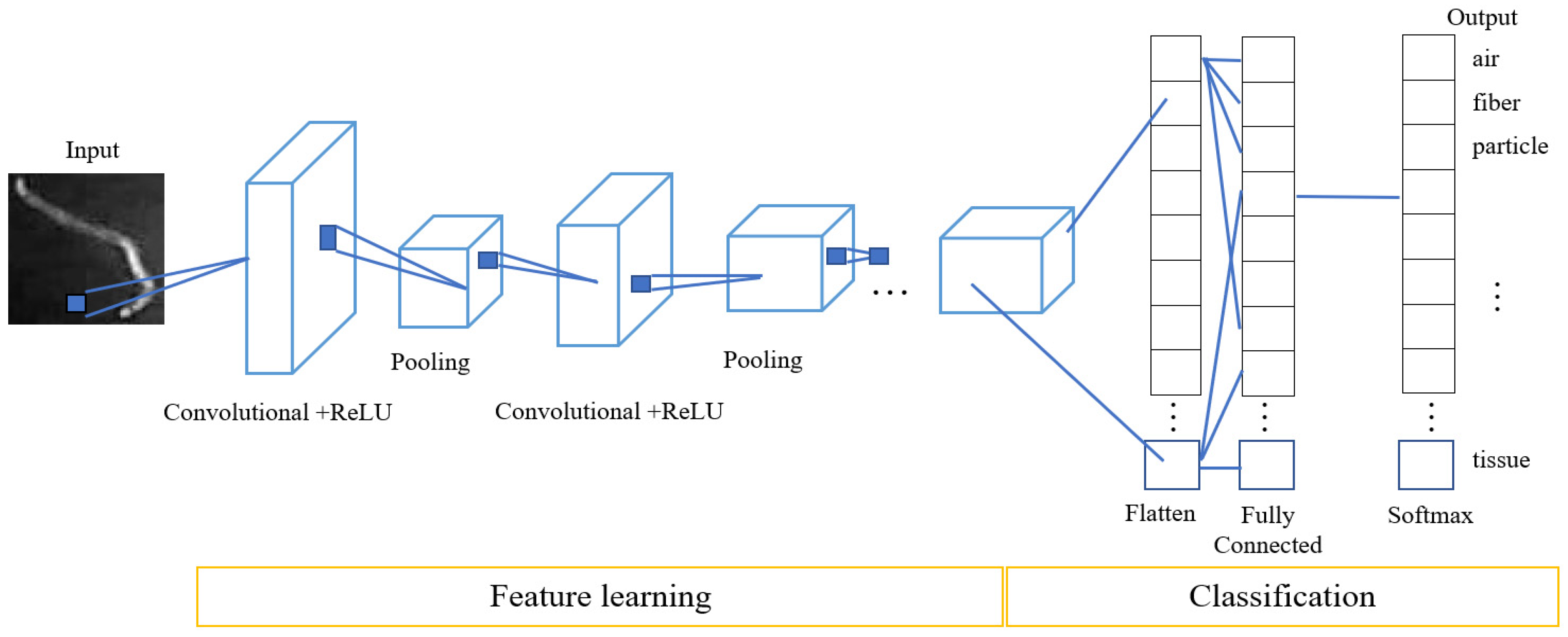
2.2. Convolutional Neural Networks
- Input layer: reads the image input data prior to passing it to the neural network.
- Convolutional layer: filters the image features from the analysis of each pixel of the image that has been read. The result is a convolutional feature map.
- Rectified linear unit (ReLU): performs a nonlinear activation function.
- Pooling layer: provides a subsample rectified feature map to reduce linear dimensions and create a feature representation.
- Softmax layer: configures the output to display it in the form of a multiclass logistic classifier.
- Output layer: displays the results of the classification.
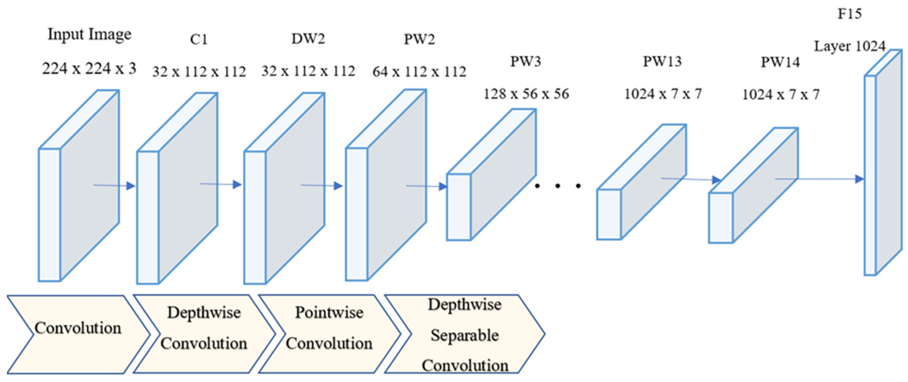
2.3. MobileNet
2.4. VGGNet
2.5. GoogLeNet
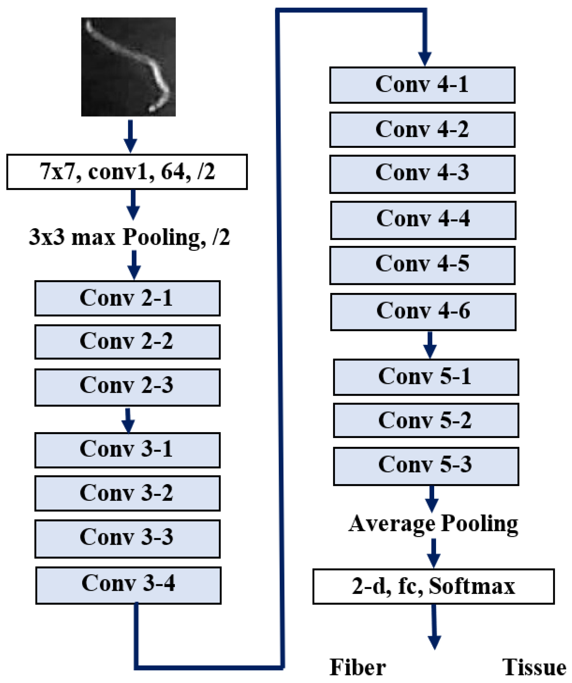
2.6. ResNet
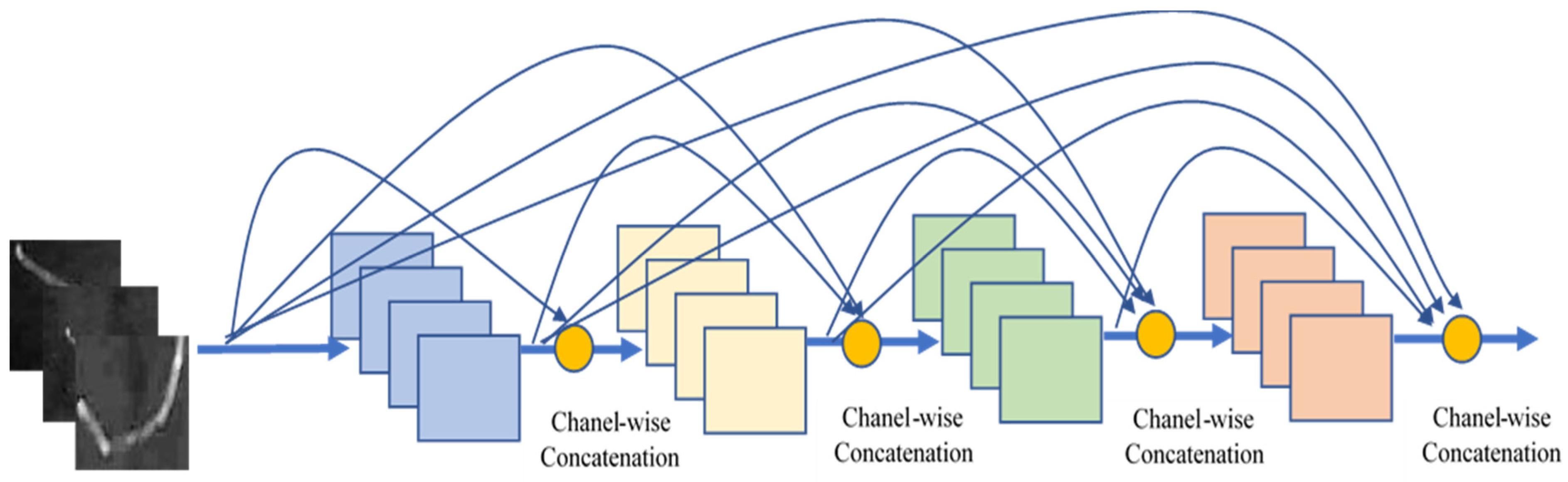
2.7. DenseNet
3. Research Methodology
3.1. Datasets
3.2. Experimental Settings and Results
3.2.1. Experiments with MobileNetV2
3.2.2. Comparison of the MobileNet and Other CNN Architectures
3.2.3. Experiments with Data Augmentation
3.3. Discussion
4. Conclusions
Author Contributions
Funding
Institutional Review Board Statement
Informed Consent Statement
Acknowledgments
Conflicts of Interest
References
- Karnawat, V.; Patil, S. Turbidity detection using image processing. In Proceedings of the 2016 International Conference on Computing, Communication and Automation (ICCCA), Greater Noida, India, 29–30 April 2016. [Google Scholar]
- Berg, M.; Videen, G. Digital holographic imaging of aerosol particles in flight. J. Quant. Spectrosc. Radiat. Transf. 2011, 112, 1776–1783. [Google Scholar] [CrossRef] [Green Version]
- Pastore, V.P.; Zimmerman, T.; Biswas, S.; Bianco, S. Annotation-free learning of plankton for classification and anomaly detection. Sci. Rep. 2020, 10, 12142. [Google Scholar] [CrossRef] [PubMed]
- Versaci, M.; Calcagno, S.; Jia, Y.; Morabito, F.C. Fuzzy Geometrical Approach Based on Unit Hyper-Cubes for Image Contrast Enhancement. In Proceedings of the 2015 IEEE International Conference on Signal and Image Processing Applications (ICSIPA), Kuala Lumpur, Malaysia, 19–21 October 2015. [Google Scholar]
- amirberAgain, Python and openCV to Analyze Microscope Slide Images of Airborne Particles. Available online: https://publiclab.org/notes/amirberAgain/01-12-2018/python-and-opencv-to-analyze-microscope-slide-images-of-airborne-particles (accessed on 25 May 2021).
- Oheka, O.; Chunling, T. Fast and Improved Real-Time Vehicle Anti-Tracking System. Appl. Sci. 2020, 10, 5928. [Google Scholar] [CrossRef]
- Dechter, R. Learning while searching in constraint-satisfaction-problems. In Proceedings of the Fifth AAAI National Conference on Artificial Intelligence (AAI’86), Philadelphia, PA, USA, 11–15 August 1986. [Google Scholar]
- Schmidhuber, J. Deep learning in neural networks: An overview. Neural Netw. 2015, 61, 85–117. [Google Scholar] [CrossRef] [Green Version]
- Fukushima, K. Recent advances in the deep CNN neocognitron. Nonlinear Theory Appl. IEICE 2019, 10, 304–321. [Google Scholar] [CrossRef]
- LeCun, Y. 1.1 Deep Learning Hardware: Past, Present, and Future. In Proceedings of the 2019 IEEE International Solid-State Circuits Conference—(ISSCC), San Francisco, CA, USA, 17–21 February 2019. [Google Scholar]
- Li, X.; Xiong, H.; An, H.; Xu, C.; Dou, D. RIFLE: Backpropagation in Depth for Deep Transfer Learning through Re-Initializing the Fully-connected LayEr. In Proceedings of the 37th International Conference on Machine Learning (ICML2020), Vienna, Austria, 12–18 July 2020. [Google Scholar]
- Ranzato, M.A.; Huang, F.; Boureau, Y.; LeCun, Y. Unsupervised learning of invariant feature hierarchies with applications to object recognition. In Proceedings of the 2007 IEEE Conference on Computer Vision and Pattern Recognition (CVPR), Minneapolis, MN, USA, 17–22 June 2007. [Google Scholar]
- Brinker, T.J.; Hekler, A.; Utikal, J.; Grabe, N.; Schadendorf, D.; Klode, J.; Berking, C.; Steeb, T.; Enk, A.; Kalle, C.V. Skin Cancer Classification Using Convolutional Neural Networks: Systematic Review. J. Med. Internet Res. 2018, 20, e11936. [Google Scholar] [CrossRef]
- Patil, R.; Bellary, S. Machine learning approach in melanoma cancer stage detection. J. King Saud Univ. Comput. Inf. Sci. 2020, in press. [Google Scholar] [CrossRef]
- Khairi, M.T.M.; Ibrahim, S.; Yunus, M.A.M.; Faramarzi, M.; Yusuf, Z. Artificial Neural Network Approach for Predicting the Water Turbidity Level Using Optical Tomography. Arab. J. Sci. Eng. 2016, 41, 3369–3379. [Google Scholar] [CrossRef]
- Newby, J.M.; Schaefer, A.M.; Lee, P.T.; Forest, M.G.; Lai, S.K. Convolutional neural networks automate detection for tracking of submicron-scale particles in 2D and 3D. Proc. Natl. Acad. Sci. USA 2018, 15, 9026–9031. [Google Scholar] [CrossRef] [PubMed] [Green Version]
- Rong, D.; Xie, L.; Ying, Y. Computer vision detection of foreign objects in walnuts using deep learning. Comput. Electron. Agric. 2019, 162, 1001–1010. [Google Scholar] [CrossRef]
- Ferreira, A.D.S.; Freitas, D.M.; Silva, G.G.D.; Pistori, H.; Folhes, M.T. Weed detection in soybean crops using ConvNets. Comput. Electron. Agric. 2017, 143, 314–324. [Google Scholar] [CrossRef]
- Krizhevsky, A.; Sutskever, I.; Hinton, G.E. ImageNet classification with deep convolutional neural networks. Commun. ACM 2017, 60, 84–90. [Google Scholar] [CrossRef]
- Simonyan, K.; Vedaldi, A.; Zisserman, A. Deep Inside Convolutional Networks: Visualising Image Classification Models and Saliency Maps. arXiv 2014, arXiv:1312.6034. [Google Scholar]
- Simonyan, K.; Zisserman, A. Very Deep Convolutional Networks for Large-Scale Image Recognition. In Proceedings of the 2015 International Conference on Learning Representations (ICLR 2015). arXiv 2014, arXiv:1409.1556. [Google Scholar]
- Howard, A.G.; Zhu, M.; Chen, B.; Kalenichenko, D.; Wang, W.; Weyand, T.; Andreetto, M.; Adam, H. MobileNets: Efficient Convolutional Neural Networks for Mobile Vision Applications. arXiv 2017, arXiv:1704.04861. [Google Scholar]
- Pan, H.; Pang, Z.; Wang, Y.; Wang, Y.; Chen, L. A New Image Recognition and Classification Method Combining Transfer Learning Algorithm and MobileNet Model for Welding Defects. IEEE Access. 2020, 8, 119951–119960. [Google Scholar] [CrossRef]
- Kerf, T.D.; Gladines, J.; Sels, S.; Vanlanduit, S. Oil Spill Detection Using Machine Learning and Infrared Images. Remote Sens. 2020, 12, 4090. [Google Scholar] [CrossRef]
- Iqbal, U.; Barthelemy, J.; Li, W.; Perez, P. Automating Visual Blockage Classification of Culverts with Deep Learning. Appl. Sci. 2021, 11, 7561. [Google Scholar] [CrossRef]
- Tammina, S. Transfer learning using VGG-16 with Deep Convolutional Neural Network for Classifying Images. Int. J. Sci. Res. Publ. 2019, 9, 143–150. [Google Scholar] [CrossRef]
- Szegedy, C.; Liu, W.; Jia, Y.; Sermanet, P.; Reed, S.E.; Anguelov, D.; Erhan, D.; Vanhoucke, V.; Rabinovich, A. Going deeper with convolutions. In Proceedings of the 2015 IEEE Conference on Computer Vision and Pattern Recognition (CVPR), Boston, MA, USA, 7–12 June 2015. [Google Scholar]
- He, K.; Zhang, X.; Ren, S.; Sun, J. Deep residual learning for image recognition. In Proceedings of the IEEE Conference on Computer Vision and Pattern Recognition, Las Vegas, NV, USA, 27–30 June 2016. [Google Scholar]
- Aparna; Bhatia, Y.; Rai, R.; Gupta, V.; Aggarwal, N.; Akula, A. Convolutional neural networks based potholes detection using thermal imaging. J. King Saud Univ. Comput. Inf. Sci. 2019, in press. [Google Scholar] [CrossRef]
- Huang, G.; Liu, Z.; Pleiss, G.; Maaten, L.V.; Weinberger, K.Q. Convolutional Networks with Dense Connectivity. IEEE Trans. Pattern. Anal. Mach. Intell. 2019, 1–12. [Google Scholar] [CrossRef] [PubMed] [Green Version]
- Tao, Y.; Xu, M.; Lu, Z.; Zhong, Y. DenseNet-Based Depth-Width Double Reinforced Deep Learning Neural Network for High-Resolution Remote Sensing Image Per-Pixel Classification. Remote. Sens. 2018, 10, 779. [Google Scholar] [CrossRef] [Green Version]
- Too, E.C.; Yujian, L.; Njuki, S.; Yingchun, L. A comparative study of fine-tuning deep learning models for plant disease identification. Comput. Electron. Agric. 2019, 161, 272–279. [Google Scholar] [CrossRef]
- Palananda, A.; Kimpan, W. Turbidity of Coconut Oil Determination Using the MAMoH Method in Image Processing. IEEE Access 2021, 9, 41494–41505. [Google Scholar] [CrossRef]

| Class | Example of Particle Image for Model Training | ||||||||
|---|---|---|---|---|---|---|---|---|---|
| Air |  |  |  |  |  |  |  |  |  |
| FiberT1 |  |  |  |  |  |  |  |  |  |
| FiberT2 |  |  |  |  |  |  |  |  |  |
| FiberT3 |  |  |  |  |  |  |  |  |  |
| FiberT4 |  |  |  |  |  |  |  |  |  |
| ParticleT1 |  |  |  |  |  |  |  |  |  |
| ParticleT2 |  |  |  |  |  |  |  |  |  |
| ParticleT3 |  |  |  |  |  |  |  |  |  |
| ParticleT4 |  |  |  |  |  |  |  |  |  |
| Tissue |  |  |  |  |  |  |  |  |  |
| Width Multipliers | Accuracy (%) | Size Model (Mb) |
|---|---|---|
| 1.00 | 94.05 | 12.52 |
| 0.75 | 88.72 | 8.38 |
| 0.50 | 71.54 | 5.60 |
| 0.25 | 74.25 | 3.88 |
| Resolution | Accuracy (%) | Size Model (Mb) |
|---|---|---|
| 224 × 224 | 94.05 | 12.52 |
| 192 × 192 | 93.40 | 12.52 |
| 160 × 160 | 92.56 | 12.52 |
| 128 × 128 | 91.22 | 12.52 |
| Resolution | Width Multipliers | |||
|---|---|---|---|---|
| 1.00 | 0.75 | 0.50 | 0.25 | |
| 224 × 224 | 94.05 | 88.72 | 71.54 | 74.25 |
| 192 × 192 | 93.40 | 88.77 | 72.35 | 74.44 |
| 160 × 160 | 92.56 | 88.21 | 71.23 | 72.87 |
| 128 × 128 | 91.22 | 87.83 | 70.96 | 73.23 |
| Predicted Class (Accuracy) | |||||||||||
|---|---|---|---|---|---|---|---|---|---|---|---|
| Actual Class | Class | Air | FiberT1 | FiberT2 | FiberT3 | FiberT4 | ParticleT1 | ParticleT2 | ParticleT3 | ParticleT4 | Tissue |
| Air | 0.81 | 0.02 | 0.02 | 0.00 | 0.03 | 0.00 | 0.07 | 0.01 | 0.04 | 0.00 | |
| FiberT1 | 0.02 | 0.83 | 0.05 | 0.01 | 0.01 | 0.03 | 0.03 | 0.00 | 0.02 | 0.00 | |
| FiberT2 | 0.00 | 0.01 | 0.92 | 0.00 | 0.00 | 0.01 | 0.04 | 0.00 | 0.01 | 0.00 | |
| FiberT3 | 0.04 | 0.09 | 0.03 | 0.72 | 0.04 | 0.01 | 0.05 | 0.00 | 0.02 | 0.01 | |
| FiberT4 | 0.01 | 0.12 | 0.05 | 0.04 | 0.62 | 0.04 | 0.08 | 0.00 | 0.04 | 0.00 | |
| ParticleT1 | 0.05 | 0.03 | 0.00 | 0.00 | 0.00 | 0.73 | 0.08 | 0.03 | 0.03 | 0.05 | |
| ParticleT2 | 0.03 | 0.03 | 0.02 | 0.00 | 0.00 | 0.00 | 0.87 | 0.04 | 0.00 | 0.00 | |
| ParticleT3 | 0.03 | 0.02 | 0.02 | 0.00 | 0.00 | 0.00 | 0.09 | 0.78 | 0.00 | 0.06 | |
| ParticleT4 | 0.02 | 0.00 | 0.00 | 0.00 | 0.00 | 0.00 | 0.00 | 0.00 | 0.98 | 0.00 | |
| Tissue | 0.05 | 0.04 | 0.02 | 0.01 | 0.00 | 0.01 | 0.11 | 0.02 | 0.00 | 0.74 | |
| No | Model | Input Resolution | Accuracy (%) Model | Training Time (Hour) | Test Time (Minute) | Size Model (Mb) |
|---|---|---|---|---|---|---|
| 1 | MobileNetV2 | 224 × 224 × 3 | 94.05 | 5.13 | 18.20 | 12.52 |
| 2 | Standard CNN | 224 × 224 × 3 | 89.70 | 1.17 | 18.35 | 8.27 |
| 3 | Xception | 299 × 299 × 3 | 92.82 | 30.08 | 22.44 | 842.33 |
| 4 | InceptionV3 | 299 × 299 × 3 | 93.23 | 15.38 | 20.22 | 96.88 |
| 5 | ResNet50 | 224 × 224 × 3 | 91.65 | 16.04 | 19.27 | 689.54 |
| 6 | ResNet101 | 224 × 224 × 3 | 90.21 | 25.42 | 19.37 | 795.23 |
| 7 | DenseNet121 | 224 × 224 × 3 | 93.53 | 21.47 | 20.10 | 827.27 |
| 8 | VGG16 | 224 × 224 × 3 | 91.95 | 8.39 | 18.56 | 689.41 |
| 9 | VGG19 | 224 × 224 × 3 | 91.12 | 12.19 | 19.55 | 722.58 |
| 10 | InceptionResNetV2 | 299 × 299 × 3 | 90.93 | 30.25 | 20.37 | 956.36 |
| No | Model | Image Input | Test Model with Confusion Matrix Form PiCO_V1 Dataset (%) | |||
|---|---|---|---|---|---|---|
| Accuracy | Precision | Recall | F1Score | |||
| 1 | MobileNetV2 | 224 × 224 × 3 | 80.20 | 71.61 | 81.15 | 76.08 |
| 2 | Standard CNN | 224 × 224 × 3 | 54.82 | 45.09 | 61.01 | 51.86 |
| 3 | Xception | 299 × 299 × 3 | 72.95 | 64.62 | 76.24 | 69.95 |
| 4 | InceptionV3 | 299 × 299 × 3 | 75.13 | 68.19 | 77.14 | 72.39 |
| 5 | ResNet50 | 224 × 224 × 3 | 68.88 | 62.12 | 72.61 | 66.95 |
| 6 | ResNet101 | 224 × 224 × 3 | 66.44 | 66.56 | 67.29 | 66.92 |
| 7 | DenseNet121 | 224 × 224 × 3 | 68.55 | 62.75 | 69.38 | 65.90 |
| 8 | VGG16 | 224 × 224 × 3 | 68.52 | 60.55 | 73.02 | 66.20 |
| 9 | VGG19 | 224 × 224 × 3 | 70.02 | 69.38 | 71.89 | 68.58 |
| 10 | InceptionResNetV2 | 299 × 299 × 3 | 55.55 | 55.25 | 58.79 | 55.44 |
Publisher’s Note: MDPI stays neutral with regard to jurisdictional claims in published maps and institutional affiliations. |
© 2022 by the authors. Licensee MDPI, Basel, Switzerland. This article is an open access article distributed under the terms and conditions of the Creative Commons Attribution (CC BY) license (https://creativecommons.org/licenses/by/4.0/).
Share and Cite
Palananda, A.; Kimpan, W. Classification of Adulterated Particle Images in Coconut Oil Using Deep Learning Approaches. Appl. Sci. 2022, 12, 656. https://doi.org/10.3390/app12020656
Palananda A, Kimpan W. Classification of Adulterated Particle Images in Coconut Oil Using Deep Learning Approaches. Applied Sciences. 2022; 12(2):656. https://doi.org/10.3390/app12020656
Chicago/Turabian StylePalananda, Attapon, and Warangkhana Kimpan. 2022. "Classification of Adulterated Particle Images in Coconut Oil Using Deep Learning Approaches" Applied Sciences 12, no. 2: 656. https://doi.org/10.3390/app12020656
APA StylePalananda, A., & Kimpan, W. (2022). Classification of Adulterated Particle Images in Coconut Oil Using Deep Learning Approaches. Applied Sciences, 12(2), 656. https://doi.org/10.3390/app12020656