A Matrix Effect Correction Method for Portable X-ray Fluorescence Data

Abstract

Portable X-ray fluorescence spectrometry (pXRF) is an analytical technique that can be used for rapid and non-destructive analysis in the field. However, the testing accuracy and precision for trace elements are significantly affected by the matrix effect, which comes mainly from major elements that constitute most of the matrix of a sample. To solve this problem, many methods based on linear regression models have been proposed, but when extreme values or outliers occur, the application of these methods will be greatly affected. In this study, 16 certified reference materials were collected for pXRF analysis, and the major elements most closely related to the elements to be measured were employed as correction indicators to calibrate the analysis results through the application of multiple linear regression analysis. Some statistical parameters were calculated to evaluate the correction results. Compared with the calibration data obtained from simple linear regression analysis without taking major elements into account, those corrected by the new method were of higher quality, especially for elements of Co, Zn, Mo, Ta, Tl, Pb, Cd and Sn. The results show that the new method can effectively suppress the influence of the matrix effect.

1. Introduction

Portable X-ray fluorescence spectrometry (pXRF) offers some unique advantages in chemical composition analysis, which arise from the multi-element capability, the non-destructive nature and the immediate availability to the researcher of information on the chemical composition of a sample in the field [1]. In addition, this technique is characterized by decreased production of hazardous waste and low running costs [2]. At present, pXRF analysis has been widely used in mineral resource exploration [3], environmental monitoring and evaluation [4], archaeological research [5], agricultural survey [6] and many other fields.

However, the matrix effect that occurs in pXRF analysis generally has a heavy influence on the quality of the analysis results, especially for trace elements [7]. The interference of the sample particle size, surface structure, chemical composition and mineral morphology on the analysis are all matrix effects [8]. In fact, the matrix influence is essentially the impact that the sample matrix has on the X-ray intensity emitted during analysis, which is mainly reflected by the absorption and enhancement or overlap in the spectral peaks [9]. As a result, matrix effect correction has been the focus of much attention, and many correction methods have been put forward from different points of view [10].

Currently, there are two kinds of correction methods for the matrix effect. One suppresses the matrix effect by experimental manipulations, such as the internal standard method, the standard addition method and the dilution method. The other eliminates the matrix effect by mathematical means, such as the linear regression method and machine learning [11]. The experimental method will, however, make the experimental process more complicated and increase the experimental workload. At present, the most commonly used correction methods are mathematical methods [12], of which most are based on the linear regression model, such as the fundamental parameter method and the experience coefficient method [13]. These methods, however, only use the element to be measured to establish a regression equation and pay little attention to the role of other elements, especially major elements that have a great influence on the determination of trace elements. For example, the element Fe will cause a significant increase in test value of Co [14], and the resulting outlier (an extremely high value) may lead to an unrealistic regression curve [15]. As for the machine learning algorithm, such as artificial neural networks [16], random forests [17] and geographically weighted regression [18], they have become an important statistical tool in dealing with pXRF data, but they are not stable and sometimes have the local optimum problem.

In this study, pXRF analysis was performed on 16 certified reference materials (CRMs), including 10 rock samples and 6 soil samples, and some major elements were selected as correction indicators to correct the analysis results with the application of a new method based on multiple linear regression analysis [19]. For comparison, the simple linear regression (SLR) method is also performed on the data. Some statistical parameters, such as the coefficient of determination (R²), mean absolute error (MAE) and root mean square error (RMSE), are calculated and discussed in detail to evaluate the performance of these two methods.

2. Materials and Methods

2.1. Samples and Analyses

A total of 16 CRMs were selected, including 10 rock samples and 6 soil samples (

Table 1. Certified reference samples for pXRF analysis.

Lithology	Number	Sample No.
Rock	10	GBW07104, GBW07105, GBW07106, GBW07107, GBW07122, GBW07162, GBW07163, GBW07165, GBW07825, ZBK336
Soil	6	GBW07401, GBW07403, GBW07404, GBW07405, GBW07406, GBW07408

Note: These samples were provided by the Institute of Geophysical and Geochemical Exploration of the Chinese Academy of Geological Science.

), for pXRF analysis, and 34 elements were detected, including Mg, Al, Si, P, S, K, Ca, Ti, Mn, Fe V, Cr, Co, Ni, Cu, Zn, As, Se, Rb, Sr, Y, Zr, Nb, Mo, Cd, Sn, Sb, Ba, Ta, W, Tl, Pb, Bi and U. The pressed powder pellet technique was used for sample preparation. The sample powder was pressed into a pellet with a diameter of 5 cm and a thickness of about 2 cm under 30 kPa for 30 s. The experimental instrument was a portable energy dispersive X-ray fluorescence spectrometer (X-MET7000) from the Oxford Instruments Group, founded in Oxford, England in 1959. The instrument had a rhodium (Rh) anode target and a fourth-generation silicon drift detector (SDD). Elements between Mg (atomic number of 12) and U (atomic number of 92) on the periodic table of elements could be analyzed [8]. The samples were determined under the conditions of a voltage of 40 kV and current of 60 mA, and each test lasted 60 s. In order to reduce the influence of sample heterogeneity, the analysis was repeated 5 times in different positions homogeneously distributed in the sample, and the average value was calculated as the final result [20].

2.2. Correction Method for the Matrix Effect

According to the Sherman equation (Equation (1)), which describes the relationship between the measured intensities emitted by a sample and its composition [21,22], the pXRF analysis result of an element is affected by all the other elements in a sample:

$$I_j=f\left(C_j,C_k,\dots ,C_m\right)$$

(1)

where I_j is the net intensity of element j, C_j is the concentration of element j and C_k–C_m are the concentrations of other elements.

However, not all elements can be determined by pXRF analysis due to the low detection limits of some elements [23]. In addition, this equation is not reversible for calculating unknown sample compositions. At present, the commonly used correction method is the regression method. Note that major components of a sample contribute most to the matrix effect and therefore should be considered important indicators in matrix effect correction, such as Si, Al, Fe, Ca, K, Mn and Ti. As a result, major elements were added as an independent variable into the commonly used SLR model, and then a multiple linear regression equation (Equation (2)) could be established [11]:

$$C_i^{\prime }={\alpha }_i{C}_i+{\alpha }_j{C}_j+u_i$$

(2)

where C_i’ is the reference value of element i, C_i and C_j are the pXRF testing values of element i and major element j that is most closely related to element i, respectively, α_i is the regression coefficient of element i, α_j is the influence coefficient of major element j to element i and u_i is the regression intercept of element i.

The values of α_i, α_j and u_i are affected by the instrument conditions and can be calculated by testing the CRMs. In this process, the ordinary least squares approach [24,25], which is one the most popular chemometric algorithms for calibration model creation, is used. Similarly, this method requires minimizing the sum of the squares of the residuals. As a result, α_i, α_j and u_i can be obtained by solving Equations (3)–(5):

$${\alpha }_i=\frac{\left({\sum }_{k=1}^n{M}_{ik}^{\prime }{M}_{ik}\right)\left({\sum }_{k=1}^n{M}_{jk}^2\right)-\left({\sum }_{k=1}^n{M}_{ik}^{\prime }{M}_{jk}\right)\left({\sum }_{k=1}^n{M}_{ik}{M}_{jk}\right)}{\left({\sum }_{k=1}^n{C}_{ik}^2\right)\left({\sum }_{k=1}^n{C}_{jk}^2\right)-{\left({\sum }_{k=1}^n{C}_{ik}{C}_{jk}\right)}^2}$$

(3)

$${\alpha }_j=\frac{\left({\sum }_{k=1}^n{M}_{ik}^{\prime }{M}_{jk}\right)\left({\sum }_{k=1}^n{M}_{ik}^2\right)-\left({\sum }_{k=1}^n{M}_{ik}^{\prime }{M}_{ik}\right)\left({\sum }_{k=1}^n{M}_{ik}{M}_{jk}\right)}{\left({\sum }_{k=1}^n{C}_{ik}^2\right)\left({\sum }_{k=1}^n{C}_{jk}^2\right)-{\left({\sum }_{k=1}^n{C}_{ik}{C}_{jk}\right)}^2}$$

(4)

$$u_i=\frac{\left({\sum }_{k=1}^n{C}_{ik}^{\prime }\right)-{\alpha }_i\left({\sum }_{k=1}^n{C}_{ik}\right)-{\alpha }_j\left({\sum }_{k=1}^n{C}_{jk}\right)}{k}$$

(5)

where n is the number of samples and $C_{ik}$ and $C_{jk}$ are the testing values of elements i and j in sample k, respectively. The testing values of i and j are zero centered to $M_{ik}$ and $M_{jk}$ by the following equation.$M_{ik}^{\prime }$ and $C_{ik}^{\prime }$ are the transposes of $M_{ik}$ and $C_{ik}$, respectively:

$$M_{ik}=C_{ik}-\frac{{\sum }_{k=1}^n{C}_{ik}}{k}$$

(6)

$$M_{ij}=C_{jk}-\frac{{\sum }_{k=1}^n{C}_{jk}}{k}$$

(7)

2.3. Parameters for Evaluation of the Correction Results

Some statistical parameters were employed to evaluate the correction results, including the coefficient of determination (R²), relative error (RE), mean absolute error (MAE), mean absolute percentage error (MAPE), root mean squared error (RMSE) and root mean square percentage error (RMSPE). The correlation between the pXRF testing value and the reference value of an element could be estimated by the R² values. The larger the R² value is, the stronger the correlation is [26]. It is generally considered that high-quality data can be obtained when the relative error (RE) does not exceed 20%. In this paper, the accuracy of the pXRF analysis was estimated by P_RE, which represents the percentage of data with an RE not exceeding 20% [26]. When the P_RE value approached 1, the testing accuracy was high, indicating that the experimental results were accurate. The parameter MAE was used to measure the average absolute error between the corrected value and the reference value of the experimental data set, and the RMSE was used to measure the deviation between the observed value and the true value [27]. As for the MAPE and RMSPE, they could be used to evaluate the relative errors and dispersion of the whole test values of a sample, respectively. The smaller the four values were, the more accurate and the less discrete the correction results were [28]. These parameters could be obtained by solving the following equations:

$$R^2=\frac{{\sum }_{k=1}^n{\left(C_{ik}^{\prime }-\overline{C_i}\right)}^2}{{\sum }_{k=1}^n{\left(C_{ik}^0-\overline{C_i}\right)}^2}$$

(8)

$$RE=\frac{\left|C_{ik}^{\prime }-C_{ik}^0\right|}{C_{ik}^0}\times 100\%$$

(9)

$$MAE=\frac{{\sum }_{k=1}^n\left|C_{ik}^{\prime }-C_{ik}^0\right|}{n}$$

(10)

$$MAPE=\frac{1}{n}\times {\displaystyle \sum }_{k=1}^n\frac{\left|C_{ik}^{\prime }-C_{ik}^0\right|}{C_{ik}^0}\times 100\%$$

(11)

$$RMSE=\sqrt{\frac{{\sum }_{k=1}^n{(C_{ik}^{\prime }-C_{ik}^0)}^2}{n}}$$

(12)

$$RMSPE=\sqrt{\frac{1}{n}\times {\displaystyle \sum }_{k=1}^n{\left(\frac{C_{ik}^{\prime }-C_{ik}^0}{C_{ik}^0}\right)}^2}\times 100\%$$

(13)

where $C_{ik}^{\prime }$ denotes the predicted value of element i in sample k by the new method or the simple linear regression method, $C_{ik}^0$ is the reference value of element i in sample k and $\overline{C_i}$ represents the average reference value of element i in all samples.

3. Results and Discussion

3.1. The pXRF Analysis Results

The pXRF analysis results and reference values of the samples are shown in Tables S1 and S2, respectively. The data were imported into OriginPro Learning Edition, and scatter plots were drawn with the testing values as the X-axis coordinate and reference values as the Y-axis coordinate (Figure 1). It can be seen that the different elements had different distribution patterns. For example, the plots of some elements show that there was almost no difference between the testing and reference values, which indicates that these elements had high testing accuracy, including Al, Si, P, S, K, Ca, Ti, Mn, Fe, Cu, Zn, As, Rb, Sr, Zr, Pb and Bi. If not strictly required, the analysis results of these elements could be used directly without correction. The plots of the other elements show that there were varying degrees of difference between their testing values and reference values, indicating that the analysis results of these elements needed to be corrected. Note that the plots of some of these elements (e.g., Mg, Ni, Y, Nb and Sb) exhibited a significant linear relationship between the testing values and reference values. Obviously, the SLR correction method could be used for these elements. However, the elements V, Cr, Co, Se, Mo, Cd, Sn, Ba, Ta, W, Tl and U did not have a linear relationship between their testing and reference values, and therefore, it made little sense to perform the SLR correction.

3.2. The Correction of the Matrix Effect

The correction indicators should be determined before using the new method for data calibration. The major elements that had the highest correlation with the element to be corrected and are not or just slightly influenced by other elements could be selected as correction indicators [10]. The results of the correlation analysis showed the major elements with the highest correlation coefficients with the elements to be corrected (

Table 2. Correction indicators for elements to be tested by pXRF analysis.

Correction Indicator	Trace Elements to Be Tested
Al	Cu, Se, Rb, Mo, Sb, Sn, W, Tl, As, Bi, U
Ti	P, Cr, Y, Zr, Nb, Ta
Fe	Mg, V, Co, Ni
Mn	Cd, Zn
Si	S, Pb
K	Ba
Ca	Sr

). The number of trace elements mostly related to Al in the pXRF analysis was the largest, reaching 11 and accounting for almost half of all the elements. The following major elements were Ti and Fe, which affected six and four elements, respectively. The elements Mn, Si, K and Ca had little effect on the other elements, and the number of elements affected by any one of them was generally less than three. The significant correlation was either reflected in similar chemical properties or in similar positions in the periodic table.

The testing values and reference values were imported into IBM SPSS Statistics 25 to calculate the coefficients of α_i, α_j and u_i for each detected element using Equations (3)–(5). Then, the correction indicators as an independent variable were substituted, along with the coefficients of α_i, α_j and u_i, into Equation (2) to form multiple linear regression equations for each element, except the indicator elements that were slightly influenced by the matrix effect (

Table 3. Correction equations for elements detected by pXRF analysis.

Element	Multiple Linear Regression Equations	Simple Linear Regression Equations
Mg	y = 1.312x − 0.019106Fe − 0.035	y = 1.299x − 0.610
Al	-	y = 0.846x − 0.037
Si	-	y = 1.052x − 0.058
P	y = 0.882x + 0.011691Ti − 0.002	y = 0.911x + 0.019
S	y = 1.136x + 0.088753Si − 1.965	y = 1.075x − 0.893
K	-	y = 0.888x + 0.005
Ca	-	y = 0.879x + 0.150
Ti	-	y = 0.828x − 0.003
V	y = 0.066x + 17.255Fe + 43.219	y = 1.107x − 47.244
Cr	y = 0.827x + 27.540Ti − 11.885	y = 0.878x + 4.045
Mn	-	y = 0.853x − 0.004
Fe	-	y = 0.935x + 1.353
Co	y = −0.172x + 5.366Fe + 5.390	y = 0.028x + 17.870
Ni	y = 0.914x + 3.297Fe − 0.558	y = 0.965x − 1.632
Cu	y = 0.928x − 10.245Al + 147.296	y = 0.928x + 54.855
Zn	y = 1.171x − 0.000Mn − 888.827	y = 1.168 x− 810.710
As	y = 1.018x − 25.559Al + 422.940	y = 1.021x + 46.514
Se	y = 1.692x − 0.406Al − 13.035	y = 2.483x − 37.067
Rb	y = 0.841x + 1.068Al − 2.205	y = 0.866x + 2.394
Sr	y = 0.787x + 0.690Ca ± 0.001	y = 0.790x + 3.256
Y	y = 0.719x − 0.357Ti + 1.495	y = 0.710x + 4.660
Zr	y = 0.814x + 0.000Ti + 14.385	y = 0.844x + 15.891
Nb	y = 0.604x + 10.429Ti − 0.092	y = 0.776x − 8.625
Mo	y = 0.340x − 0.172Al − 1.664	y = 0.333x − 10.07
Cd	y = 1.879x + 331.155Mn − 13.213	y = 1.737x − 113.910
Sn	y = 0.635x + 4.047Al − 6.683	y = 0.494x − 1.312
Sb	y = 1.110x − 5.948Al − 106.578	y = 1.088x − 59.504
Ba	y = 0.069x + 596.818K − 566.860	y = 0.076x + 270.120
Ta	y = 0.033x + 1.880Ti + 4.516	y = 0.038x − 0.070
W	y = 0.286x + 4.809Al − 9.415	y = 0.360x + 3.3911
Tl	y = 1.199x + 23.460Al − 59.340	y = 0.011x + 0.554
Pb	y = 1.314x − 9284.000Si + 3365.584	y = 1.381x − 540.560
Bi	y = 4.199x + 0.428Al − 5.591	y = 2.358x − 13.724
U	y = 0.7463x − 0.006Al − 0.641	y = 0.739x − 7.474

Note: x and y represent the testing and regression values of the element to be tested, respectively. The unit is the same as in Figure 1.

). The reference value and the testing value were used as an independent variable and dependent variable, respectively. For comparison, the SLR method was also performed on the pXRF analysis results of the CRMs, and the testing and reference values of each element were used to establish regression equations (Table 3). Subsequently, both the multiple and simple linear regression equations were used to calculate the regression values for each element. The corresponding scatter plots of the regression values vs. reference values are shown in Figure 2.

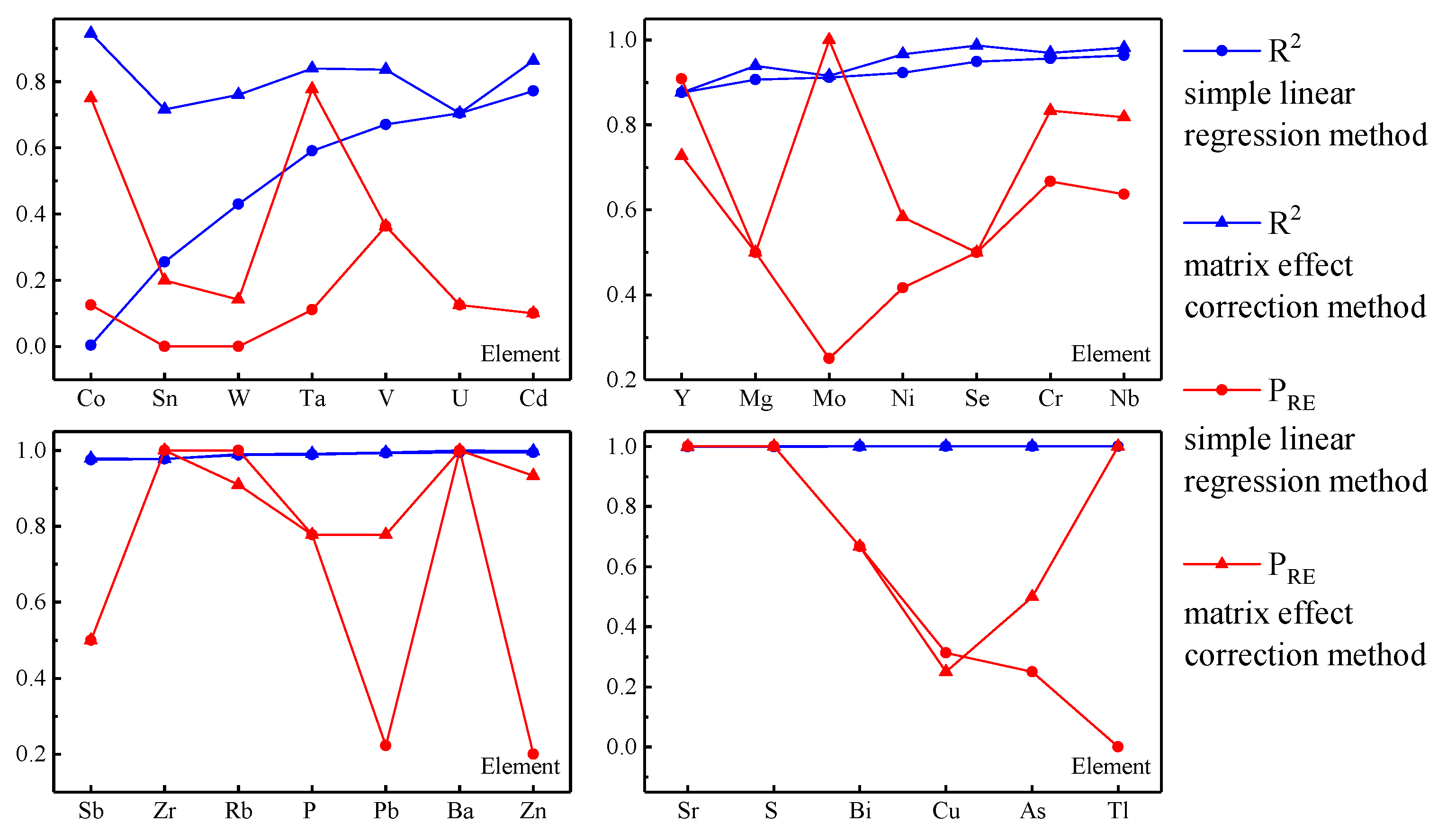
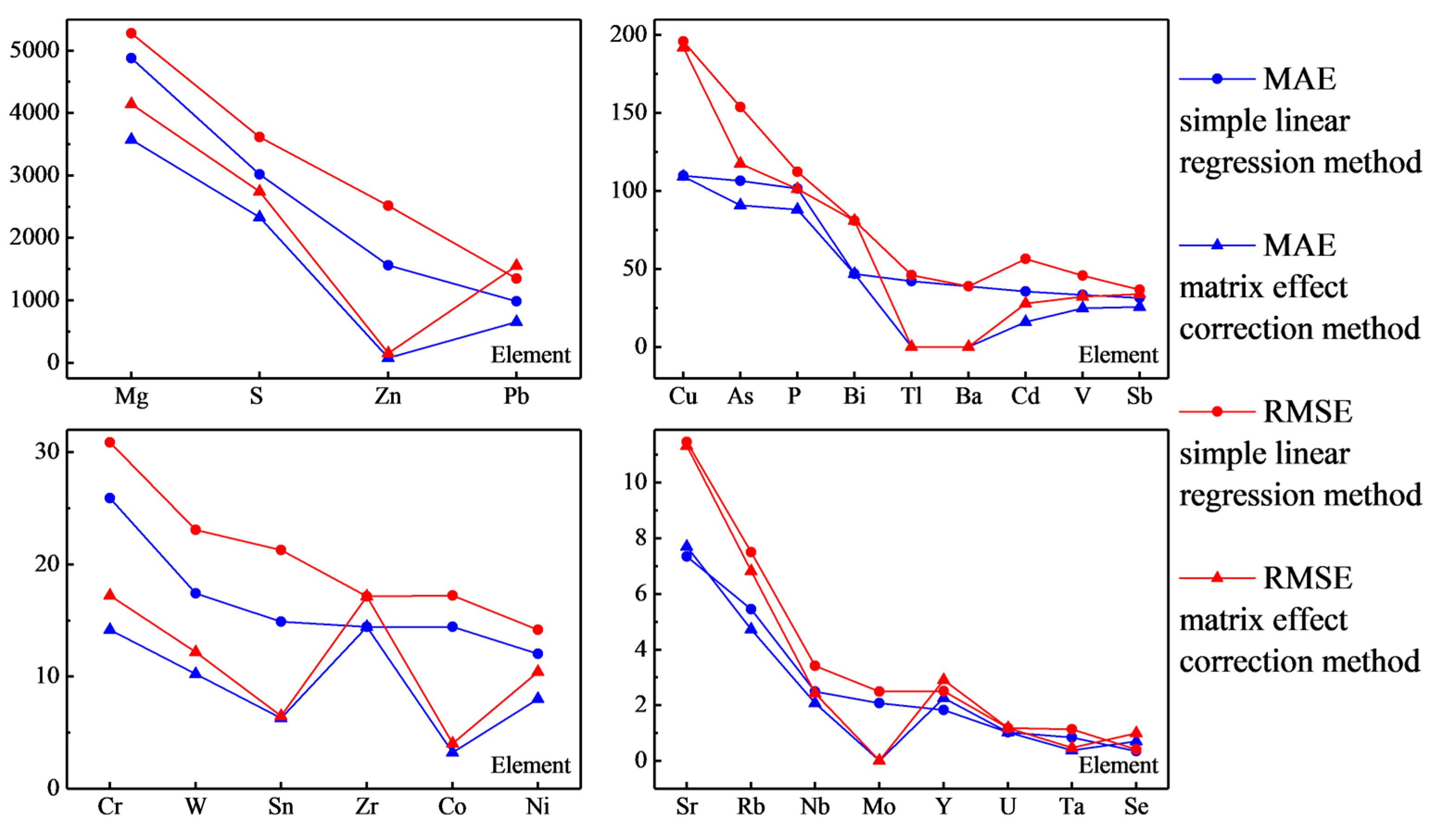
3.3. Evaluation of the Correction Results

3.3.1. Different Correction Effects

The regression results show that the matrix effect correction (MEC) and SLR methods had different correction effects on V, Cr, Co, Mo, Cd, Sn, Ta and W. It can be seen that their regression values calculated by the SLR method were quite different from their reference values, while the results of the MEC method were much closer (Figure 2), indicating that the MEC method was better than the SLR method. The statistical parameters of R², P_RE, MAE, MAPE, RMSE and RMSPE were calculated for the detected elements to evaluate the correction effect of these two methods. Not surprisingly, the MEC method had large R² values, P_RE values close to one and small MAE, MAPE, RMSE and RMSPE values (Figure 3, Figure 4 and Figure 5), while the results for the SLR method were the opposite.

Compared with the other detected elements, these elements were more closely related to the major elements, including Fe, Mn, Ti and Al, mainly due to their adjacent positions in the periodic table and similar chemical properties. As a result, the determination of these elements may inevitably have been affected by major components during pXRF analysis. In fact, the influence of the matrix effect mainly comes from the absorption or enhancement of the characteristic X-ray fluorescence intensity of the element to be tested by adjacent elements, especially major elements. These elements have low contents and weak characteristic X-ray fluorescence intensities, which may exacerbate the influence of the matrix effect.

Generally, the influence of the matrix effect can give rise to some extremely large or small testing values called outliers during the pXRF analysis, which will deviate significantly from the changing trend of normal points (Figure 2). For example, the testing values of Co were much higher than its reference values, which may have been caused by the enhancement of the characteristic X-ray fluorescence intensity by Fe (Figure 2). The testing values of V and Cr, however, were lower than their reference values, which may have been caused by the absorption of secondary X-ray fluorescence by Fe and Ti, respectively (Figure 2). If the outliers are not omitted from the analysis results before SLR regression analysis, a realistic regression curve will not be established, and therefore, the resulting regression values will also be unreliable. Note that even if the outliers are eliminated before SLR regression analysis, a realistic regression curve cannot be obtained because the testing values involved in the regression analysis are incomplete, which will affect the use of the regression equation. Obviously, this is not a fundamental solution; in other words, the influence of the matrix effect cannot be eliminated by the SLR method.

Fortunately, the MEC method can use the data of the major elements to modify the data of the outliers and, to a certain extent, weaken the influence of the matrix effect. For example, the testing values of Co, V and Cr were significantly corrected by the participation of Fe and Ti. The quality of these element data was significantly improved by the MEC method. Compared with the SLR method, the new method had better statistical parameters for all of these elements (Figure 3, Figure 4 and Figure 5). For example, all statistical parameters of Co, Mo, Sn and Ta were greatly improved. As for Cr, W, V and Cd, only a part of the parameters was enhanced; that is, the R² and P_RE values of Cr and W increased significantly, and the MAE, MAPE, RMSE and RMSPE values of V and Cd decreased significantly. The reason for the incomplete correction may be that these elements are also greatly affected by other elements aside from the selected major elements.

3.3.2. Similar Correction Effect

As for the other elements, these two methods had similar correction effects. However, some of these elements were well corrected, including Al, Si, P, S, K, Ca, Ti, Mn, Fe, Cu, Zn, As, Rb, Sr, Zr, Pb, Mg, Ni, Y, Nb, Sb and Bi, and some were not, including Se, Ba, Tl and U. It can be seen that there was no significant difference between the SLR and MEC regression values of the former group of elements, all of which were close to their reference values (Figure 2), indicating that these two regression methods both had a good correction effect.

However, it should also be noted that the MEC method did not play a significant role in eliminating the matrix effect for these elements, which may be because they were just slightly affected by the matrix effect. For example, although some trace elements had much lower contents and weaker characteristic X-ray fluorescence intensities than the major elements, as long as they were just slightly affected by the matrix effect, a good correction effect could also be obtained, such as the elements Rb, Sr, Zr, Ni, Y, Nb and Sb. As for the elements Al, Si, P, S, K, Ca, Ti, Mn, Fe, Cu, Zn, As, Pb and Mg, they could produce an extremely high intensity of characteristic X-ray fluorescence under X-ray irradiation due to their high contents in the certified reference samples, and therefore, other elements would have little impact on them. The statistical parameter results show that these two methods both had large R² values close to one and small MAE, MAPE, RMSE and RMSPE values (Figure 3, Figure 4 and Figure 5), which also indicate good correction effects.

For the correction of Ba, Tl, Se and U, neither of these two methods worked, and their regression values were quite different from their reference values (Figure 2). The testing accuracy of these elements was low, and there was no linear relationship between their testing values and reference values (Figure 1), which may be the reason for the poor correction effect of the SLR method. As for the MEC method, the poor correction effect may be attributed to the fact that these elements are influenced not only by the selected major elements but also by other elements or factors. Nevertheless, compared with the SLR method, the new method had better statistical parameters for Ba and Tl (Figure 3, Figure 4 and Figure 5). For example, the MAE, MAPE, RMSE and RMSPE values of Ba and Tl decreased significantly. As for Se and U, there was almost no difference between the parameters.

Regardless of whether the element was affected by the matrix effect, the new method could attain a considerable correction effect, indicating that a lot of the matrix effect was stripped off. Compared with the SLR method, the regression values of the elements V, Cr, Ta and W obtained from the new method were closer to their reference values, especially for elements Co, Mo, Cd and Sn (Figure 2). As for the elements slightly or not affected by the matrix effect, these two regression methods had considerable and almost the same correction effects. Collectively, the SLR method tends to deal with the matrix effect at a macro level without exploring the relationship between elements, while the new method has a better correction result for the matrix effect with the aid of the major elements.

4. Conclusions

In this study, 16 certified reference materials were determined by pXRF analysis, and major elements were used to calibrate the analysis results with the application of multiple linear regression analysis. The results show that the major components of a sample contributed the most to the matrix effect and could be used as important indicators in matrix effect correction. The regression method based on the correction indicators of major elements can significantly improve pXRF analysis results. Although pXRF analysis is not a substitute for laboratory analysis methods, such as X-ray fluorescence analysis, inductively coupled plasma mass spectrometry analysis and other forms of high-precision analysis, the data can provide reliable material composition information after correction.

References

1. Jinke, G.; Jilong, L.; Yechang, Y.; Yuyan, Z.; Xiaodan, T.; Yuchao, F.; Yan, L. Application of Portable XRF in Core Geochemical Characteristics of Qujia Gold Deposit in Jiaodong Area. Spectrosc. Spectr. Anal. 2020, 40, 1461–1466. [Google Scholar] [CrossRef]
2. Rawal, A.; Chakraborty, S.; Li, B.; Lewis, K.; Godoy, M.; Paulette, L.; Weindorf, D.C. Determination of base saturation percentage in agricultural soils via portable X-ray fluorescence spectrometer. Geoderma 2019, 338, 375–382. [Google Scholar] [CrossRef]
3. Zhang, W.; Lentz, D.R.; Charnley, B.E. Petrogeochemical assessment of rock units and identification of alteration/mineralization indicators using portable X-ray fluorescence measurements: Applications to the Fire Tower Zone (W-Mo-Bi) and the North Zone (Sn-Zn-In), Mount Pleasant deposit, New Brunswick, Canada. J. Geochem. Explor. 2017, 177, 61–72. [Google Scholar] [CrossRef] [Green Version]
4. Kazimoto, E.O.; Messo, C.; Magidanga, F.; Bundala, E. The use of portable X-ray spectrometer in monitoring anthropogenic toxic metals pollution in soils and sediments of urban environment of Dar es Salaam Tanzania. J. Geochem. Explor. 2018, 186, 100–113. [Google Scholar] [CrossRef]
5. Holcomb, J.A.; Karkanas, P. Elemental mapping of micromorphological block samples using portable X-ray fluorescence spectrometry (pXRF): Integrating a geochemical line of evidence. Geoarchaeology 2019, 34, 613–624. [Google Scholar] [CrossRef]
6. Pessanha, S.; Marguí, E.; Carvalho, M.L.; Queralt, I. A simple and sustainable portable triaxial energy dispersive X-ray fluorescence method for in situ multielemental analysis of mining water samples. Spectrochim. Acta Part B At. Spectrosc. 2019, 164, 105762. [Google Scholar] [CrossRef]
7. Declercq, Y.; Delbecque, N.; De Grave, J.; De Smedt, P.; Finke, P.; Mouazen, A.M.; Nawar, S.; Vandenberghe, D.; Van Meirvenne, M.; Verdoodt, A. A Comprehensive Study of Three Different Portable XRF Scanners to Assess the Soil Geochemistry of An Extensive Sample Dataset. Remote Sens. 2019, 11, 2490. [Google Scholar] [CrossRef] [Green Version]
8. Durance, P.; Jowitt, S.M.; Bush, K. An assessment of portable X-ray fluorescence spectroscopy in mineral exploration, Kurnalpi Terrane, Eastern Goldfields Superterrane, Western Australia. Appl. Earth Sci. 2014, 123, 150–163. [Google Scholar] [CrossRef]
9. West, M.; Ellis, A.T.; Potts, P.J.; Streli, C.; Vanhoof, C.; Wegrzynek, D.; Wobrauschek, P. Atomic spectrometry update—X-ray fluorescence spectrometry. J. Anal. At. Spectrom. 2012, 27, 1603–1644. [Google Scholar] [CrossRef]
10. Ang, J. Development of X-ray Fluorescence Spectrometry in the 30 Years. Rock Miner. Anal. 2012, 31, 383–398. [Google Scholar] [CrossRef]
11. Haijun, Q.; Jianying, W.; Xuefeng, Z.; Yang, W. Matrix Effect of Fe and Ca on EDXRF Analysis of Ce Concentration in Bayan Obo Ores. Spectrosc. Spectr. Anal. 2015, 35, 3510–3513. [Google Scholar] [CrossRef]
12. Song, L.; Bomin, S.; Qinghui, L.; Fuxi, G. Application of Calibration Curve Method and Partial Least Squares Regression Analysis to Quantitative Analysis of Nephrite Samples Using XRF. Spectrosc. Spectr. Anal. 2015, 35, 245–251. [Google Scholar] [CrossRef]
13. Gallhofer, D.; Lottermoser, B. The Influence of Spectral Interferences on Critical Element Determination with Portable X-ray Fluorescence (pXRF). Minerals 2018, 8, 320. [Google Scholar] [CrossRef] [Green Version]
14. Ziyue, N.; Jiwen, C.; Mingbo, L.; Xueliang, L.; Shaocheng, H. Interference correction of energy dispersive X-ray fluorescence spectrometric determination of chromium and manganese in soil. Metall. Anal. 2016, 36, 10–14. [Google Scholar] [CrossRef]
15. Tingting, G.; Ye, T.; Qian, C.; Boyang, X.; Fuzhen, H.; Lintao, W.; Ying, L. Matrix Effect and Quantitative Analysis of Iron Filings with Different Particle Size Based on LIBS. Spectrosc. Spectr. Anal. 2020, 40, 1207–1213. [Google Scholar] [CrossRef]
16. Andrade, R.; Silva, S.H.G.; Weindorf, D.C.; Chakraborty, S.; Faria, W.M.; Guilherme, L.R.G.; Curi, N. Tropical soil order and suborder prediction combining optical and X-ray approaches. Geoderma Reg. 2020, 23, e00331. [Google Scholar] [CrossRef]
17. Benedet, L.; Nilsson, M.S.; Silva, S.H.G.; Pelegrino, M.H.P.; Mancini, M.; Menezes, M.D.; Guilherme, L.R.G.; Curi, N. X-ray fluorescence spectrometry applied to digital mapping of soil fertility attributes in tropical region with elevated spatial variability. An. Acad. Bras. Cienc. 2021, 93, 4. [Google Scholar] [CrossRef] [PubMed]
18. Qu, M.; Liu, H.; Guang, X.; Chen, J.; Zhao, Y.; Huang, B. Improving correction quality for in-situ portable X-ray fluorescence (PXRF) using robust geographically weighted regression with categorical land-use types at a regional scale. Geoderma 2021, 409, 115615. [Google Scholar] [CrossRef]
19. Fragkaki, A.G.; Farmaki, E.; Thomaidis, N.; Tsantili-Kakoulidou, A.; Angelis, Y.S.; Koupparis, M.; Georgakopoulos, C. Comparison of multiple linear regression, partial least squares and artificial neural networks for prediction of gas chromatographic relative retention times of trimethylsilylated anabolic androgenic steroids. J Chromatogr. A 2012, 1256, 232–239. [Google Scholar] [CrossRef]
20. Xiaoyong, T.; Xiaofang, N.; Zhaocong, S. Effect and Correction of Iron in Soil on Accuracy of Chromium Determination by Portable X-ray Fluorescence Spectrometry. Rock Miner. Anal. 2020, 39, 460–474. [Google Scholar] [CrossRef]
21. Rousseau, R.M. Some considerations on how to solve the Sherman equation in practice. Spectrochim. Acta Part B At. Spectrosc. 2004, 59, 1491–1502. [Google Scholar] [CrossRef]
22. Rousseau, R.M. Corrections for matrix effects in X-ray fluorescence analysis—A tutorial. Spectrochim. Acta Part B At. Spectrosc. 2006, 61, 759–777. [Google Scholar] [CrossRef]
23. Fen, G.; Liang, G.; Xiaoxu, P.; Jin, Y.; Yufang, Z.; Zheng, W. Matrix Effect of Soil Samples in Laser Ablation-Atmospheric Pressure Glow Discharge Atomic Emission Spectrometry. Chin. J. Anal. Chem. 2020, 49, 1111–1119. [Google Scholar] [CrossRef]
24. Balabin, R.M.; Safieva, R.Z.; Lomakina, E.I. Comparison of linear and nonlinear calibration models based on near infrared (NIR) spectroscopy data for gasoline properties prediction. Chemom. Intell. Lab. Syst. 2007, 88, 183–188. [Google Scholar] [CrossRef]
25. Subedi, S.; Fox, T.R. Predicting Loblolly Pine Site Index from Soil Properties Using Partial Least-Squares Regression. For. Sci. 2016, 62, 449–456. [Google Scholar] [CrossRef] [Green Version]
26. Rongxi, K.; Wenyou, H.; Yue, H.; Biao, H.; Yanqun, Z.; Yuan, L.; Fangdong, Z.; Xiaoleng, Z.; Bao, W. Application of Portable X-ray Fluorescence (PXRF) for Rapid Analysis of Heavy Metals in Agricultural Soils Around Mining Area. Soils 2015, 47, 589–595. [Google Scholar] [CrossRef]
27. Cort, J.W.; Matsuura, K. Advantages of the mean absolute error (MAE) over the root mean square error (RMSE) in assessing average model performance. Clim. Res. 2005, 30, 79–82. [Google Scholar] [CrossRef]
28. Shuang, L.; Tiankai, Z.; Linzi, F. Analysis of Urban Green Development and Influencing Factors in Yangtze River Economic Belt. Stat. Decis. 2019, 35, 125–128. [Google Scholar] [CrossRef]
Figure 1. Scatter plots of testing values vs. reference values of the detected elements. The unit of Mg, Al, Si, P, S, K, Ca, Ti, Mn, Fe, Cu, Zn, As and Pb was 10−2, and that of V, Cr, Co, Ni, Se, Rb, Sr, Y, Zr, Nb, Mo, Cd, Sn, Sb, Ba, Ta, W, Tl, Bi and U was 10−6.
Applsci 12 00568 g001
Figure 2. Scatter plots of the new method and the simple linear regression method. The unit is the same as in Figure 1.
Applsci 12 00568 g002
Figure 3. The R2 and PRE values for the correction results of the new and SLR methods.
Applsci 12 00568 g003
Figure 4. The MAPE and RMSPE values for the correction results of the new and SLR methods.
Applsci 12 00568 g004
Figure 5. The MAE and RMSE values for the correction results of the new and SLR methods.
Applsci 12 00568 g005